Abstract
The South Aral Sea has been massively affected by the implementation of a mega-irrigation project in the region, but ground-based observations have monitored the Sea poorly. This study is a comprehensive analysis of the mass balance of the South Aral Sea and its basin, using multiple instruments from ground and space. We estimate lake volume, evaporation from the lake, and the Amu Darya streamflow into the lake using strengths offered by various remote-sensing data. We also diagnose the attribution behind the shrinking of the lake and its possible future fate. Terrestrial water storage (TWS) variations observed by the Gravity Recovery and Climate Experiment (GRACE) mission from the Aral Sea region can approximate water level of the East Aral Sea with good accuracy (1.8% normalized root mean square error (RMSE), and 0.9 correlation) against altimetry observations. Evaporation from the lake is back-calculated by integrating altimetry-based lake volume, in situ streamflow, and Global Precipitation Climatology Project (GPCP) precipitation. Different evapotranspiration (ET) products (Global Land Data Assimilation System (GLDAS), the Water Gap Hydrological Model (WGHM)), and Moderate-Resolution Imaging Spectroradiometer (MODIS) Global Evapotranspiration Project (MOD16) significantly underestimate the evaporation from the lake. However, another MODIS based Priestley-Taylor Jet Propulsion Laboratory (PT-JPL) ET estimate shows remarkably high consistency (0.76 correlation) with our estimate (based on the water-budget equation). Further, streamflow is approximated by integrating lake volume variation, PT-JPL ET, and GPCP datasets. In another approach, the deseasonalized GRACE signal from the Amu Darya basin was also found to approximate streamflow and predict extreme flow into the lake by one or two months. They can be used for water resource management in the Amu Darya delta. The spatiotemporal pattern in the Amu Darya basin shows that terrestrial water storage (TWS) in the central region (predominantly in the primary irrigation belt other than delta) has increased. This increase can be attributed to enhanced infiltration, as ET and vegetation index (i.e., normalized difference vegetation index (NDVI)) from the area has decreased. The additional infiltration might be an indication of worsening of the canal structures and leakage in the area. The study shows how altimetry, optical images, gravimetric and other ancillary observations can collectively help to study the desiccating Aral Sea and its basin. A similar method can be used to explore other desiccating lakes.
1. Introduction
Lakes and reservoirs store 87% of the Earth’s total fresh open water [1]. Unfortunately, many of them are gradually receding over the years due to climatic or/and anthropogenic forcings [2]. There are several feedbacks between the lake and its environment. Thus, quantifying the changes in the lake is critical to understanding the interactions among various components of the region better. For example, fluctuations in a lake/reservoir can be linked to different climatic changes at a regional scale, including desertification, dust storms, melting of glaciers, and changes in the vegetation and land types. For instance, lake volume loss reduces its heat capacity, and thus it can warm up and cool off faster than before.
One of the examples of massive lake volume reduction is the Aral Sea. In the 1960s, Soviet Russia started the world’s second largest irrigation program, under which the Amu Darya and the Syr Darya rivers were diverted across the Karakum desert. The average annual combined pre-irrigation streamflow of the Amu Darya and the Syr Darya into the Aral Sea was 56 km3 [3], which was reduced to less than 10 km3 by 2002 [4]. The world’s fourth-largest freshwater lake (until the 1960s) eventually separated into two parts, the vast South Aral Sea located in the south and the small North Aral Sea situated in the north. After the construction of Dike Kokaral dam between the north and south part of the Aral Sea, the Syr Darya streamflow has stabilized the North Aral Sea. However, in the past few decades, the perennial Amu Darya has transformed to an intermittent river as it runs through the desert and Khorezm oasis before merging into the South Aral Sea [5]. Consequently, the South Aral Sea continued its journey of desiccation and became a hypersaline and almost non-habitable lake. The Aral Sea is in the lowland climate zone [6], but studies have suggested that it may move towards a monsoon climate [4], which is characterized by seasonal climate change due to warming and cooling of the Aral Sea.
Hydrologic analysis of the Aral Sea and surrounding regions has been an active area of research in the last two decades [7,8,9,10,11]. The present study tries to advance previous studies by quantifying different hydrological parameters of the lake using various remote-sensing datasets that can complement each other. This is an essential step as in situ observations are limited and often not available. A comprehensive analysis of the dynamics of the South Aral Sea is performed using a mass balance equation as an example of how integrated multisensor data can be used to monitor different hydrological variables in an endorheic basin. This study demonstrates a framework of how a lake volume calculated from different remote-sensing data can act as a thermometer of the hydrological state of the basin. Lake volume variations are used to estimate evaporation loss from the lake, and to evaluate existing evaporation products, which are hard to validate otherwise. Furthermore, we estimated runoff from two different methods. Runoff is a product of hydrological processes acting in the watershed. To evaluate the cause of change in runoff, the saptio-temporal changes of the entire basin are analyzed.
2. Study Area
Here we study the South Aral Sea (Figure 1, blue polygon) and the Amu Darya basin (Figure 1, green polygon). The South Aral Sea is a remnant of the vast Aral Sea where the Amu Darya terminates. It has a shallow, broad east lobe and a deep, elongated west lobe, and a narrow channel connects them towards the north. The Amu Darya primarily runs through Turkmenistan and Uzbekistan covering an area of nearly 617,000 km2. It receives water almost entirely from glaciers in the Pamir Mountains and the Hindu Kush and mainly originates from Tajikistan and northern Afghanistan, forming the border between the two countries. The high Pamir and Tian Shan ranges are significantly wet, creating massive glaciers and snowfields, and the Amu Darya streamflow brings the water to the severely arid southeast of the Aral Sea. The streamflow from these glaciers is heaviest during the spring thaw.
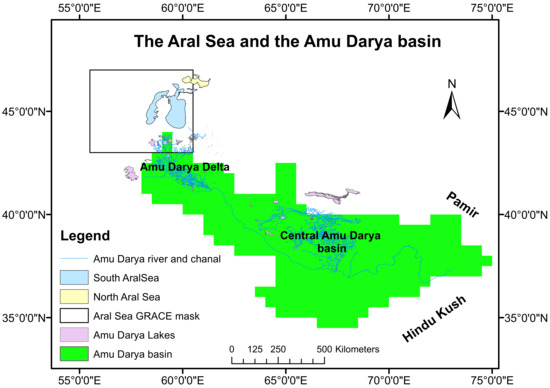
Figure 1.
Study area: the Amu Darya originates from the glaciers of Hindukush and Pamir and terminates into the South Aral Sea (blue polygon).
The Amu Darya basin mask is derived from the global river basin database obtained from http://www.wsag.unh.edu/Stn-30/stn-30.html [12,13]. The South Aral Sea land-water mask time series are generated from the multi-temporal Landsat dataset [14].
3. Observation and Model Data
3.1. Lake Water Storage (LWS)
Remote-sensing-based lake-water-storage estimation can be done using altimetry and optical images. Since 1992, satellite altimetry is used successfully for monitoring the water levels of large rivers, lakes, and floodplains [15,16,17]. Satellite altimetry measures the water surface height along its pass based on the reflection from the ground of the emitted radiations from the satellite. Different missions have different pass location, repeat cycle, and footprints. However, there are significant inter-pass gaps, which lead to limited coverage of the terrestrial water bodies. For instance, the East Aral Sea could not have reliable altimetry observations for more than four years (2012–2016) as none of the altimetry mission’s pass was over the dry lake. Singh et al. (2015) demonstrated the use of Landsat and bathymetry to obtain the water level, as an alternative to altimetry. In this study, a linear regression between altimetry water level and the Gravity Recovery and Climate Experiment (GRACE) terrestrial water storage (TWS) is examined as another alternative to estimate water level (discussed in Section 4.1).
Many studies intersected the digital elevation model (DEM) with the water level obtained from satellite altimetry to compute water storage changes of a lake/reservoir [18,19,20]. In this study also, the South Aral Sea volumetric variations are estimated by intersecting the Aral Sea bathymetry with the satellite altimetry water level time-series obtained from the Database for Hydrological Time Series of Inland Waters (DAHITI), developed by the Technische Universität München (http://dahiti.dgfi.tum.de/en/) [21]. Jason-1, Jason-2, and Jason-3, (10 days repeat pass) observe the East Aral Sea, while the West Aral Sea has additional observations from Envisat and Saral/Altika (35 days repeat pass).
Multiple Landsat missions’ (Thematic Mapper (TM), Enhanced Thematic Mapper Plus (ETM+), and Operational Land Imager (OLI)) near-infrared (NIR) images are mosaiced and classified to generate land-water mask time series. Landsat bathymetry intersection is used to create water level time-series (Singh et al. 2015).
3.2. Terrestrial Water Storage (TWS)
Since 2002, variations in the terrestrial water storage within the Earth’s system is routinely observed by GRACE [22,23,24]. The availability of monthly observations from the time variable GRACE mission has revolutionized the hydrological estimations by providing a possibility for the closure of water budget over a study area. In this study, 0.5°-gridded, JPL mascon solutions are downloaded from https://podaac.jpl.nasa.gov [25,26,27]. The mascon cell size varies with latitude, and for this region, it is 4° × 5°. Thus the GRACE signal includes mass changes occurring in the large extended area (4° × 5°) as shown in Figure 1 (black box). The study uses GRACE signals from the lake region (Figure 1, black box) to estimate its water level. However, the lake area is less than one-tenth of the area observed by GRACE, but lake volume is a major driver in the mass variation of the region. Additionally, the GRACE signal from the Amu Darya basin is also analyzed to examine the spatiotemporal pattern of the basin and to estimate long-term streamflow into the East Aral Sea. For the analysis of the Amu Darya basin, the GRACE mascon solution is scaled to sub mascon 0.5° resolution by multiplying it with 0.5° gain factor obtained from https://podaac.jpl.nasa.gov. These gain factors derived from the Community Land Model do not have a lake component. Therefore, we can not use the scaled mascon product for the lake analysis, and the mass conservation within a mascon unit is more reliable than in 0.5° sub-mascon level.
3.3. Vegetation Index
The global Moderate-Resolution Imaging Spectroradiometer (MODIS) based normalized difference vegetation index (NDVI) product (MYD13C2) is retrieved from the National Aeronautics and Space Administration (NASA) Land Processes Distributed Active Archive Center (LP DAAC) https://lpdaac.usgs.gov/ [28].
3.4. Evapotranspiration (ET)
Since 2002, the MODIS satellite has been providing a wide range of information about global dynamics at 250 m to 1 km spatial resolution. The spectral signatures captured by its 36 spectral bands are used for many applications such as optical imaging of the Earth, estimation of radiation budget, and calculation of vegetation indices. The study investigated two MODIS derived ET products: MOD16 and Priestley-Taylor Jet Propulsion Laboratory (PT-JPL).
Global monthly 0.5° MOD16 ET product is downloaded from http://ntsg.umt.edu/project/modis/mod16.php [29,30]. The MOD16 algorithm [31] is based on the Penman–Monteith (1965) equation for ET.
The PT-JPL actual evapotranspiration (AET) product [32] is based on the Priestley-Taylor potential evapotranspiration (PET) formulation. To reduce PET to AET, Fisher et al. introduced ecophysiological constraint functions based on atmospheric moisture (vapor pressure deficit and relative humidity) and vegetation indices (NDVI and soil-adjusted vegetation index). The driving equation in the model is the following:
where ETs, ETc, and ETi are evaporation from the soil, canopy and intercepted water, respectively. Each is calculated explicitly based on relative surface wetness, green canopy fraction, plant temperature constraint, plant moisture constraint and soil moisture constraint. No calibration or site-specific parameters are required for this approach.
In addition to MODIS-derived ET, we have also evaluated ET from global hydrological models (GHMs). Monthly ET estimates from the Water Gap Hydrological Model (WGHM) obtained by personal contact and the National Oceanic, and Atmospheric Administration’s (NOAA) Global Land Data Assimilation System (GLDAS) is retrieved from the http://disc.sci.gsfc.nasa.gov/ [33,34].
3.5. In Situ Data
The Aral Sea was one of the well-sampled inland water bodies on the planet until the 1980s. However, following the collapse of the USSR, field research into its advanced stages of desiccation has reduced significantly [4]. The Amu Darya monthly streamflow (2003–2010) and the historical annual hydrological data of the lake (1780–2009) are obtained from the http://www.cawater-info.net/ database. The Aral Sea bathymetry (from the 1960s) at 1 m contour spacing is provided by Prof. Renard [35] by personal communication. The East Aral Sea section of the bathymetry is updated to 30 m spatial resolution by Singh et al. [36] by combining Landsat and altimetry, and it is publicly available. Therefore, in this study, the West Aral Sea analysis is done using 1960s bathymetry while the East Aral Sea analysis used the updated bathymetry of Singh et al.
3.6. Precipitation
Monthly precipitation estimates are obtained from the latest Global Precipitation Climatology Center (GPCC V6) [37], and Global Precipitation Climatology Project (GPCP V2.3), and 1° daily data are retrieved from https://www.esrl.noaa.gov/ [38,39].
All datasets (except streamflow, Landsat, and altimetry) are harmonized to monthly, mm level water height on 0.5° (180° meridian) grid. Landsat-based 30 m resolution masks of the East and West Aral Sea are resampled to a 0.5° grid. The land-water mask time series is interested in the respective monthly evaporation and precipitation data to estimate the volumetric variations in evaporation and precipitation only from the water body.
4. Methods and Results
In this section, we demonstrate how remote-sensing observations are used to quantify the water budget components of the Aral Sea and Amu Darya basin. The retrieval method, challenges, solutions, and results are discussed as follows:
4.1. South Aral Sea Volume Dynamics
For hundreds of years (historical records began in the 1780s) until the 1960s, the Aral Sea level fluctuation was less than 5 m (Figure 2a). However, predominantly due to the massive irrigation project in the 1960s, it receded in shape and size dramatically. By 1985, the small North Aral Sea separated from the vast South Aral Sea. The North Aral Sea went through some fluctuations as seen in Figure 2a (red plot) due to many failed dam-building attempts between the two parts of the Aral Sea. It eventually stabilized after the construction of dike Kokaral dam in 2005 (Figure 2a, magenta plot). However, the South Aral Sea continued to shrink and further separated into the shallow East Aral Sea and the deep West Aral Sea by 2003 [9].
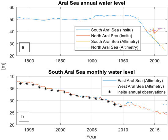
Figure 2.
Water level above mean sea level (a) historical annual Aral Sea data (b) altimetry-based monthly South Aral Sea observations.
The annual water level of the South Aral Sea was estimated by a set of altimetry sensors (i.e., Jason1, Jason2, Envisat and Saral/altika) and compared with the available in situ water level. The results show a good agreement (Figure 2a) with more than 0.99 correlation and ~60 cm RMSE (root mean square error) or 1.8% normalized RMSE (by the mean of the observed data). Figure 2b (red and blue plots) shows that East and West Aral Sea had similar water level until 2009 and they were disconnected for the first time in late 2009. However, the 2010 flood resumed the equipotential status between the two parts of the South Aral Sea for nearly a year. Afterward, they started their independent paths of desiccation. The reason behind their different progression since 2010 has been that the East Aral Sea reached approximately its lake bed later in 2009, so it needs to rise for about 2 m to get reconnected with the West Aral Sea. The West Aral gets water only from the East Aral overflow; there was a 3–4 months lag between the increase in water level in 2010 among the two parts. Meanwhile, the West Aral continuously undergoes evaporation loss, as its lakebed is 13 m below mean sea level (MSL), while the flat East Aral dries up at 27 m.
Satellite altimetry missions have continuously observed the West Aral Sea. However, the East Aral Sea lacks reliable observations after its water level went below 28.5 m (Figure 2b, red plot) because none of the altimetry missions has passed through the dry lake. Therefore, other remote-sensing observations have to be explored to explain the missing water level for nearly four years from 2011. Singh et al. (2015) demonstrated that Landsat together with bathymetry can provide 0.97 correlation with the altimetry water level and can act as a good alternative. However, optical images fail in bad weather (dust storm, and cloud). Consequently, observations from Landsat are not available for many months, especially during winters over the Aral Sea (Figure 3b). Therefore, we examined another potential way to fill the gaps by linear regression between GRACE-based terrestrial water storage (TWS) from the Aral Sea region (Figure 1). Study area black box) and the East Aral Sea water level from altimetry. First, seasonal components from the TWS and water level time series are removed. Then deseasonalized TWS and water level (Figure 3a) are linearly regressed using nine years (2003–2011) of monthly data. The best fit model (r2 = 0.82, RMSE = 49 cm) is used for the estimation of the deseasonalized water level for the 2003–2017 time frame, and then the altimetry-based seasonal component is added. The derived GRACE-based water level and altimetry observations showed 0.9 correlation and ~54 cm RMSE or 1.8% normalized RMSE. Figure 3b shows that GRACE-based estimates agreed well with the altimetry observations except for the 2010 flood. The GRACE-based estimate observed an early peak in spring 2010, while altimetry saw it in summer 2010. It can be attributed to the integral nature of the GRACE signal, which observes mass changes not only from the surface water but also from the soil moisture and groundwater.
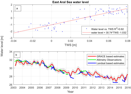
Figure 3.
The East Aral Sea water level. (a) Best fit between de-seasonalized terrestrial water storage (TWS) and altimetry water level; and (b) altimetry water level observations compared with the derived water height from Landsat and Gravity Recovery and Climate Experiment (GRACE). The gray area shows the uncertainty range of the GRACE-based estimate, calculated by the ± root mean square error (RMSE).
Although the TWS variability in this mascon also includes signals from the West Aral Sea, it obtains water only from the East Aral Sea overflow. Therefore, the empirical relation between the increase in the TWS and water level of the East Aral Sea remains valid. The East Aral acquires a similar water surface area as the West Aral as soon as it floods due to its flat topography and eventually has similar evaporation loss progression. However, the impact of consecutive evaporation loss from the West Aral on TWS may lead to the overestimation of the water-level drop, but it soon reaches the cutoff as the East Aral dries up. Therefore, the GRACE-derived sea level for the East Aral Sea stops at 27 m, as in late 2014, and it resumes with an increase in the TWS of the lake. Whenever the two parts of the South Aral are connected, then they have mostly similar progression but different water levels since 2010.
However, due to the limited spatial resolution of GRACE, the GRACE mask (Figure 1, black box) extends beyond the lake. Spring 2010 was relatively wet, (which increased the soil moisture in the entire 4° × 5° box and the lake size was at its diminished level. It seems that whenever snow accumulation or soil moisture variation is more than lake mass change, TWS has less ability to estimate the water level. Furthermore, the GRACE mask also includes the Amu Darya delta, which absorbs a significant amount of the floodwater before it reaches the South Aral Sea (discussed in Section 4.2). Figure 3b also shows that in spring 2009, GRACE-based estimates were nearly 29.5 m, which cannot be correct because there is no altimetry observation for that period, suggesting that water level had to be below 28.5 m. In this case, the time series is interpolated to fill the data gaps.
Nevertheless, for rest of the time-series, TWS in the GRACE box is driven by the lake mass variation, and thus the GRACE-based water level shows good agreement with altimetry observations.
Figure 3b shows the complete disappearance of the East Aral Sea in 2014, consistent with the analysis of the Landsat data (Singh et al. 2016). The East Aral Sea bed is approximately 27 m above MSL, and when its water level reaches 28.5 m from MSL, the lake expands enough to be observed by altimetry missions. Therefore, to obtain a complete time series, the water level is estimated from a combination of altimetry (when the water level is above 28.5 m) and Landsat (when the water level is below 28.5 m). GRACE-based estimates are used when neither altimetry nor Landsat could is available.
In this study, we have three independently generated datasets of lake structure. Lake level is estimated by satellite altimetry, lake water-surface-area or contours are estimated by the Landsat imageries and bathymetry of the lake derived from 1960s field observations. A combination of any of the two can calculate the third, for example, the altimetry and Landsat/MODIS combination can generate the bathymetry of a lake [36,40] or estimate lake volume from [18,41]. In this work, the bathymetry of the East and West Aral Sea are intersected with their respective water levels to obtain water surface area time-series due to data gaps in the Landsat observations (Figure 3b). Volumetric variations of the lakes are calculated using a truncated pyramid model (Equation (2)) by integrating the change in water level and surface area [18].
where,
- = Volumetric variations with respect to the initial state (t0) at the nth month
- = Area of the water extent at month t
- = Area of the water extent at the previous month
- = Level of the water body at month t
- = Level of the water body at the previous month.
- n = Number of months.
Between 1993 and 2017, the South Aral Sea lost approximately 195 km3 water (Figure 4a). Since 2009, the East Aral Sea has been fluctuating on its almost flat lakebed. Eventually, most of the streamflow evaporates within a year. The West Aral Sea seasonally receives some water when the East Aral Sea water level exceeds 28.5 m above MSL. However, due to evaporation loss, the West Aral Sea was still losing water at approx. 2.7 km3/annum rate and reduced below 25 m by late 2016 (Figure 2b). Considering the geometry of the West Aral Sea (Figure 4b), nearly 43 km3 of its volume might still exist below the 25 m water level. If the current trend of water loss (almost 2.7 km3/year) continues, then the West Aral Sea might disappear by nearly 2032. The seasonal expansion and shrinking of the East Aral Sea are neither enough to revive the east part nor maintain the West Aral Sea due to massive evaporation loss. The South Aral Sea dynamics are driven by the Amu Darya streamflow and evaporation loss from the lake. Therefore, we further explored these two parameters.
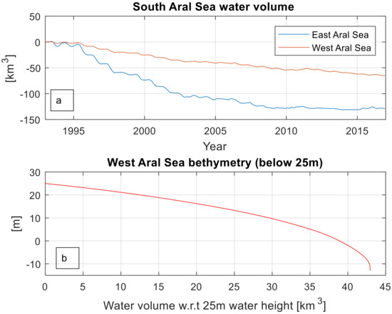
Figure 4.
(a) the South Aral Sea volume variations and (b) the West Aral Sea bathymetry below 25 m MSL.
4.2. Evaporation from the South Aral Sea
The Aral Sea is a terminal inland water body, and evaporation is the only major water outlet. The annual evaporation rate of the lake was nearly 66 km3 [9] before the 1960s. The historical vertical flux data from the Aral Sea shows a substantial difference between the total annual precipitation and evaporation to/from the waterbody (Figure 5a). However, the recent annual fluxes from the lake shown in Figure 5b demonstrate that MOD16 ET is almost equal to GPCP precipitation. It cannot be realistic, knowing the fact that the lake is shrinking and it has an additional Amu Darya streamflow into it.
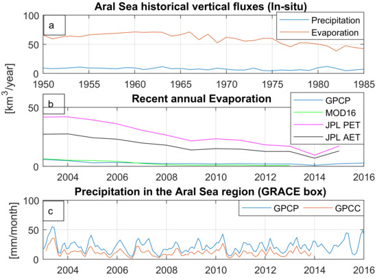
Figure 5.
Time series of the South Aral Sea precipitation and evaporation; (a) historical annual in-situ observations; (b) recent annual evapotranspiration (ET) and Global Precipitation Climatology Project (GPCP) observations; and (c) monthly precipitation observations over the lake.
Figure 5b shows that the difference between annual AET and PET has decreased due to accelerated AET with the decreasing lake size. The positive feedback between sea surface temperature (SST) and evaporation can explain the increase in the rate of AET from the Aral Sea. As the lake loses water, it not only reduces water surface area but also becomes shallower. Shallow water like the shrunken East Aral Sea (especially since 2009) heats up faster than deep water as it has less volume per square area. With decreasing lake area, specific humidity near the lake surface is decreased, and thus the rate of evaporation is increased. Another distinguishing factor of the East Aral Sea is its increasing salinity, which is above 130 ppm [10]. The salinization of the lake leads to vertical stratification, which is characterized by a rapid change in water temperature and salinity level at a given horizontal or vertical region. Consequently, the surface of the lake heats up faster as the salt concentration is not distributed evenly but stratified from lower salt concentration at the surface to the highest at the bottom of the lake [42].
Considering the significance of the evaporation for the water balance of the Aral Sea, we compared potential ET from PT-JPL, and actual ET estimates from WGHM, GLDAS, MOD16, and PT-JPL for the South Aral Sea.
Evaporation from open water is considerably different from land. Terrestrial open water evaporation dynamics needs to be added in the current evaporation estimates taking into account the land-water conversion. The presence of a lake and its size have a significant impact on its surrounding climate. Total evaporation decreases with the reducing size of the lake, but most of the ET models do not use a dynamic water mask. Consequently, the impact of available water in the system can be miscalculated. In this study, the time-variable Landsat-based water-surface masks are intersected with all the ET estimates to calculate volumetric evaporation loss from the waterbody.
As an independent estimate of evaporation, we back-calculated evaporation from the lake using lake volume dynamics (Figure 4a) and based on the water balance equation (Equation (3)):
where,
- BCE = Back-calculated evaporation from the lake (magenta plot in Figure 6)
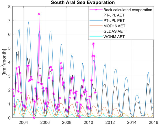 Figure 6. Evaporation from the South Aral Sea back-calculated evaporation (BCE) compared with the other ET products.
 - = Diffrential of the lake volume (calculated by Equation (2)) with respect to its previous month
- R = Amu Darya streamflow into the South Aral Sea
- P = Precipitation
This alternative and independent approach to calculate the lake evaporation provides an additional tool for evaluating the evaporation products. However, groundwater infiltration into the lake has been ignored in this estimation due to non-availability of the data. The lake volume estimates have limited uncertainty compared to other hydrological parameters because of the well-established water level estimation methods from satellite altimetry with cm-level accuracy [21]. However, the bathymetry of the lake is more than half a century old, and it has experienced some restructuring due to floods [18]. This may introduce an unknown uncertainty (likely to be small) in the estimation of the lake volume. Nevertheless, the estimated lake volume variations can be considered as a strong constraint in the water balance equation.
Additional uncertainty in back-calculated evaporation (BCE) comes from the lack of the exact coordinate of the streamflow gauge, which measures Amu Darya streamflow into the Aral Sea. The Amu Darya terminates in a massive delta with many small lakes. During the low/normal flow, water reaches directly into the East Aral Sea. However, during heavy streamflow (2005 and 2010) a significant amount of water is consumed in the delta region. Therefore, except during the flood months, the BCE can be considered as the nearest approximation of the evaporation loss from the South Aral Sea. The BCE estimates (Figure 6, magenta plot) are limited by the availability of the streamflow data (until 2010).
Precipitation is relatively a smaller direct input in the region with 80–200 mm annual range [43]. GPCP observations are closer to this range compared to GPCC (Figure 5c). Therefore, for the back-calculation of evaporation from the lake (Equation (3)), GPCP is used. Furthermore, GPCP utilizes the nearest rain-gauge stations to reduce potential biases. Figure 6 shows that most of the products severely underestimate ET compared to the BCE estimation. The PT-JPL ET, however, indicates notably different and reasonable agreement with the BCE.
The BCE shows an even better agreement with the PT-JPL AET given a month’s time lag because the BCE is estimated based on changes in the lake volume compared to its previous month. Except for the flooding months, the PT-JPL AET shows 0.83 correlation with the BCE and 0.76 cubic km RMSE (42% NRMSE). Theoretically, AET should be similar to PET over open water, but we found that they differ because a lot of the radiation/energy to drive ET gets absorbed deep into the water without actually ever evaporating any water. Therefore, the actual ET ends up being less than the potential. The MOD16 and GHMs ET showed very low seasonality in the lake volume estimation. Thus, our analysis indicates that PT-JPL ET is more consistent with the rest of the water cycle component for the evaluation of evaporation over the open water. PT-JPL has been widely and independently assessed as the top-performing global ET remote-sensing algorithm for evaporation [44,45,46,47,48,49,50,51]. However, this paper is the first to compare it with other ET products over open water. This shows that PT-JPL probably has a good representation of surface-atmosphere moisture coupling.
4.3. Amu Darya Streamflow into the Lake
As global lakes are not always well instrumented, this analysis provides insights on how well streamflow might be estimated using other water-cycle components. The study attempted to determine the Amu Darya streamflow into the South Aral Sea by two independent methods.
- A water balance-based streamflow estimate (R1, Figure 7b, green plot) is generated by combining PT-JPL ET (assuming it as actual evaporation from the lake), GPCP and South Aral Sea volumetric variations (Equation (4)). The average annual Amu Darya streamflow into the lake (except 2005 and 2010 flow) ranges between 0–1 km3/month while the accumulated error from different datasets in Equation (4) is more than one km3/month. Consequently, accurate estimation of the streamflow is not possible with this method. Therefore, three-monthly weighted-average (3MWA) by 0.25, 0.5, 0.25 weights, is calculated to obtain a long-term trend of the streamflow into the lake. The derived estimate (R1, Figure 7b) showed 0.71 correlation with the in situ 3MWA streamflow.where,
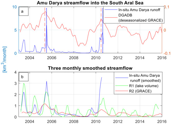 Figure 7. The Amu Darya streamflow. (a) Deseasonalized GRACE signal from the Amu Darya basin (DGADB) compared with the in-situ streamflow. The red vertical lines are peaks of DGADB, and the blue vertical lines are peaks of in situ streamflow; (b) three monthly-smoothed Amu Darya streamflow observed by in situ data compared with the two derived estimates (R1 and R2).
- R1 = Streamflow estimated from lake water budget (green plot in Figure 7b)
- 3MWA = three-monthly weighted-average
- ET = Evaporation from the lake (PT-JPL ET) and P = Precipitation (GPCP)
- Second streamflow (R2, Figure 7b, red plot) is calculated from the deseasonalized GRACE signal obtained from the Amu Darya basin (DGADB) (Figure 1, green polygon). An empirical relation between 3MWA of the in-situ Amu Darya streamflow and 3MWA of the DGADB is used to generate GRACE-based streamflow (R2). The Least-absolute-residuals method based two-degree polynomial curve showed a good agreement (r2 = 0.94 and RMSE = 0.2 km3) between the two. The derived curve (R2, Figure 7b) showed 0.68 correlation with the in situ 3MWA streamflow.
Furthermore, the dashed vertical lines in Figure 7a shows that the DGADB observes flood peaks into the lake about two months earlier than the in situ data (compare red and blue dashed lines). Reager et al. [52] also demonstrated that basin-scale TWS could be used to characterize regional flood potential with longer lead times in flood warnings. This two months’ early warning of heavy streamflow into the Amu Darya delta could be useful for the water resource management of the region.
As discussed above, the streamflow during the flood events (2005 and 2010) was significantly absorbed in the massive Amu Darya delta. Therefore, the estimated R1 and R2 have a relatively smaller peak in 2005 and 2010 than in situ streamflow. Figure 7b suggests that R1 and R2 provide only a general idea of the long-term trend and are likely to be far from true streamflow. However, they have captured well the extreme weather events in the long-term patterns of the streamflow into the lake, i.e., 2005 and 2010 floods and 2009 and 2014 droughts. R2 produces low flow reasonably well (except in 2004), but underestimates peak flow, yet the pattern of the peak flow is captured. R1 is relatively skillful in capturing peak flows but overall provides many false signals not observed by either in situ observation or GRACE. The GRACE signal (DGADB, Figure 7a red plot) indicates that 2015 and 2016 had high seasonality, but they do not exceed 2005/2010 peak flows or 2009/2014 low flows.
4.4. The Amu Darya Basin
Figure 8 shows the spatiotemporal linear trend in the Amu Darya basin between 2003 and 2017 of (a) TWS from GRACE, (b) precipitation from GPCP, (c) MODIS NDVI and (d) ET from MOD16. The figure shows that during this period TWS went down in the Amu Darya delta and the southwestern Hindukush region. The decrease in the delta TWS can be attributed to the increasing absorption of water in the central and northeastern part of the Amu Darya basin. This area is a major irrigation belt (other than a delta region) of the basin. The figure shows that in the irrigation area water mass increased (Figure 8a), ET decreased (Figure 8d), and the precipitation trend remained relatively flat (Figure 8b), which indicates a possible increase in infiltration. Furthermore, a decrease in total annual Amu Darya streamflow into the Aral Sea from more than 10 km3 in 2002 to less than 4 km3 by 2009 shows that either precipitation has gone down during those years (which is not seen in GPCP dataset) or abstraction of water has increased upstream. On the other hand, the reduction of NDVI in the central part of the basin (Figure 8c) supports the assumption of increased infiltration loss. However, vegetation loss can also be attributed to increasing salt deposition in the soil profiles and desertification [8]. Forkutsa et al. [53] discussed the fact that more than 40% of the river water is lost to evaporation and infiltration from the canal. Water escapes the route to form lakes and ponds along the way. Consequently, the rise in groundwater level has brought soil salt to the surface, leading to widespread salinization [9]. It is probable that during this time frame the canal conditions are deteriorated, leading to more infiltration loss.
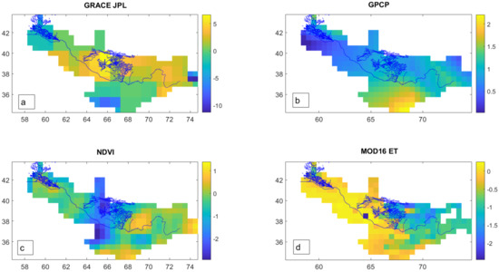
Figure 8.
The Amu Darya basin: (a) GRACE TWS; (b) GPCP; (c) normalized difference vegetation index (NDVI); and (d) MODIS based ET (MOD16).
5. Discussion
Accurate monitoring of the world’s lakes in a changing climate is increasingly essential, as lakes often significantly contribute to regional climatology and ecosystems. Several lakes are drying (e.g., Aral Sea, Urmia, Lake Chad) due to climate change and anthropogenic activities (e.g., through water abstractions for irrigation). These not only lead to loss of Lake Habitat and biodiversity but also can trigger several adverse impacts on the environment and life in the surrounding region, like desertification, dust storms, and the salinization of land. All these processes can eventually offset economic growth near the lakes. Similar processes can be seen in various global lakes like Lake Urmia [54,55], Lake Chad [56,57], the Dead Sea [58,59,60], and Lake Poopo [61,62]. Therefore, careful monitoring of the changes in lake/inland sea properties is becoming critical more than ever. Unfortunately, many of these lakes are not well instrumented. Thus exploiting the potential of integrating multi-dimensional remote-sensing data with other complementary data is essential. The following are the highlights of this research:
- Lake level estimate: this paper suggests methods for filling gaps in the altimetry observations. These data gaps may occur due to intermission time lag or loss of altimetry ground track due to changes in the shape of the water bodies. Landsat images together with bathymetry can provide an alternative water level estimate. However, sometimes, optical images have limitations during lousy weather. In that case, GRACE signals from lakes like the Aral Sea have a potential to estimate water level. The linear regression between the TWS and water level has been explored to generate the water level from GRACE.
- The rate of evaporation loss: most of the models/data products do not estimate evapotranspiration (ET) from inland waterbodies well, except for one. We have back-calculated the lake evaporation (BCE) by integrating altimetry-based lake volume variations, with the in situ runoff and GPCP precipitation. This study found the PT-JPL ET estimate to have the closest approximation to the BCE compared to the other existing ET products MODIS (MOD16) and hydrological models (WGHM and GLDAS). While PT-JPL has never been tested over open water bodies, our findings are consistent with multiple studies that have consistently found PT-JPL to be the top-performing ET remote-sensing algorithm over terrestrial vegetation [44,45,48,49,51,63].
- Estimating river streamflow to the lake: the study also suggests that the GRACE signal from the Amu Darya basin can provide a long-term trend of streamflow into the lake and may predict flood events one or two months in advance. Another streamflow is estimated based on the lake water budget, which showed a good long-term progression but has some false highs. The back-calculated streamflow (R1) indicated strikingly high seasonality, which demonstrates possible seasonal groundwater infiltration into the lake, assuming error in other datasets are not seasonally biased. Nevertheless, in the absence of any in-situ streamflow, these methods can be explored.
- Assessing the spatiotemporal variations in the water cycle of the Amu Darya basin: finally, we monitored the spatial changes of the Amu Darya basin to examine the cause of reducing streamflow. Various insights could be gained through analyzing the maps of a temporal trend in ET, TWS, NDVI, and Precipitation. The decrease in TWS in the Amu Darya delta region is mainly due to the increase in water mass in the central part of the Amu Darya basin, which is probably due to rising infiltration with the worsening of the canal system. This assumption cannot be validated due to lack of ground-based observations but is supported by the decrease in ET and NDVI in the region with the increase in TWS.
- Future of the Aral Sea: the low Amu Darya streamflow and huge evaporation loss from the vast open body have endangered the existence of the South Aral Sea. If the present trend continues, the remnant West Aral Sea will also disappear by nearly 2032 or reach the level of its base flow. One possible solution is to drain the Amu Darya streamflow directly into the West Aral Sea to avoid evaporation loss from the vast shallow East Aral Sea. Assuming 4 km3/year water flows into the West Aral Sea based on the current the annual Amu Darya streamflow (without any flood), the West Aral Sea will start increasing at a rate of more than 1 km3/year. Additionally, a dam is also required to be built between the East and West Aral Sea to stop flooding from the west when it reaches more than 28 m above MSL.
6. Concluding Remarks
In this paper, we show how the combination of various remote-sensing products can help gain more information on the fate of the Aral Sea lake. A framework that can be extended to study other endorheic lakes. The Aral Sea was well instrumented in the Soviet era, after which it gradually lost ground-based stations. However, some in situ records for streamflow to the lake (until 2010), and lake bathymetry (from the 1960s) are available. These enable us to assess current remote-sensing potential and determine challenging areas for further improvement. Our study over the Aral Sea mainly consists of using remote-sensing data to quantify changes in the lake level and volume, the rate of evaporation loss, estimating river streamflow to the lake, and assessing the spatiotemporal variations in the water cycle of both the lake and the Amu Darya basin. The study demonstrated that in addition to altimetry, optical and GRACE data can help to estimate the lake level. Also, GRACE may predict flood events one or two months in advance. Furthermore, lake evaporation was calculated using runoff, altimetry, and precipitation. In comparison to the other global ET products (for example WGHM, GLDAS, MOD16), PT-JPL ET showed the best approximation to the estimated ET for the open water. The Aral Sea basin analysis by the GRACE and other datasets suggests a rise in infiltration, potentially due to worsening of the canals.
Efforts are ongoing to monitor other world’s inland lake. Given the lack of quality in situ observations, remote sensing has shown great potential. However, several areas require further improvement by the community, some of which are highlighted below:
- Higher spatial resolution GRACE signals can improve its application tremendously by reducing the impact of contributions from other hydrological compartments.
- Evaporation estimates from the waterbodies need to be better estimated. The lake’s volume variations and its salinity need to be incorporated in the models.
- With the recent operation of Global Precipitation Measurements (GPM) and Soil Moisture Active Passive (SMAP) missions, precipitation, soil moisture is expected to be monitored better than before. The role of new observations in studies like that presented here needs to be further investigated.
- The upcoming Surface Water and Ocean Topography (SWOT) mission is expected to provide volumetric variations of most of the inland water bodies because of its wide swath altimetry. This can potentially advance water balance studies such as that investigated in this work.
- By increasing confidence in the quality of surface/sub-surface estimates (surface water and soil moisture), the role of groundwater dynamics can be better explored from GRACE.
The study demonstrated the potential of deriving some proxy estimates of the missing or inadequate hydrological variables by combining multi-dimensional, multi-sensor and multi-mission earth observation datasets to undertake a comprehensive analysis of the hydrological state of a basin.
Author Contributions
The study was conceptualized and investigated by A.S. She prepared the original draft and took care of modifications. A.B. is the principal investigator of the project. He consistently improved the work by important guidance, ideas, and effective discussions. J.B.F. contributed to the paper by providing the PT-JPL data and its analysis. A.B. and J.B.F. helped in the improvement of the original draft by thorough revisions. J.T.R. and A.B. provided funding for the project. All the co-authors assisted in the finalization of the manuscript.
Acknowledgments
Authors acknowledge different agencies for proving various data, including NASA Physical Oceanography Distributed Active Archive Center (PO.DAAC) for GRACE TWS, NASA Land Process Distributed Active Archive Center (LP DAAC) for NDVI, Numerical Terradynamic Simulation Group for MOD16, Cawater group for the Aral Sea in-situ data, DAHITI for altimetry data, NASA Goddard Earth Sciences Data and Information Services Center (GES DISC) for GLDAS ET, NOAA’s Earth System Research Laboratory for GPCP and GPCC data. The authors are thankful to Prof. Andreas Guentner (GFZ, Potsdam) for proving WGHM data. Gregory Halverson processed the PT-JPL ET data. The research described in this paper was carried out at the Jet Propulsion Laboratory, California Institute of Technology, under a contract with the National Aeronautics and Space Administration. Financial support was also made available from NASA GRACE, and GRACE-FO (NNH15ZDA001NGRACE) and NASA Energy and Water Cycle Study, (NH13ZDA001N-NEWS) awards; J.B.F. was also supported by NASA SUSMAP. Government sponsorship is acknowledged.
Conflicts of Interest
The authors declare no conflict of interest. The founding sponsors had no role in the design of the study; in the collection, analyses, or interpretation of data; in the writing of the manuscript, and in the decision to publish the results.
References
- Gleick, P.H.; Pacific Institute for Studies in Development, Environment; Security, Stockholm Environment Institute. Water in Crisis: A Guide to the World’s Fresh Water Resources; Oxford University Press: New York, NY, USA, 1993; ISBN 978-0-19-507627-1. [Google Scholar]
- Nicholson, S.E. Historical Fluctuations of Lake Victoria and Other Lakes in the Northern Rift Valley of East Africa. In Environmental Change and Response in East African Lakes; Lehman, J.T., Ed.; Springer Netherlands: Dordrecht, The Netherlands, 1998; Volume 79, pp. 7–35. ISBN 978-90-481-5043-4. [Google Scholar]
- Bortnik, V.N.; Chistyaeva, S.P. Hydrometeorology and Hydrochemistry of the USSR Seas. Aral Sea Leningr. Gidrometeoizdat 1990, VII, 196. [Google Scholar]
- Zavialov, P.O. Physical Oceanography of the Dying Aral Sea; Springer Science & Business Media: Berlin, Germany, 2005; ISBN 978-3-540-22891-2. [Google Scholar]
- Dodson, J.; Betts, A.V.G.; Amirov, S.S.; Yagodin, V.N. The nature of fluctuating lakes in the southern Amu-dar’ya delta. Palaeogeogr. Palaeoclimatol. Palaeoecol. 2015, 437, 63–73. [Google Scholar] [CrossRef]
- Micklin, P.P. The Water Management Crisis in Soviet Central Asia. Carl Beck Pap. Russ. East Eur. Stud. 1991, 131. [Google Scholar] [CrossRef]
- Asokan, S.M.; Rogberg, P.; Bring, A.; Jarsjö, J.; Destouni, G. Climate model performance and change projection for freshwater fluxes: Comparison for irrigated areas in Central and South Asia. J. Hydrol. Reg. Stud. 2016, 5, 48–65. [Google Scholar] [CrossRef]
- Bosch, K.; Erdinger, L.; Ingel, F.; Khussainova, S.; Utegenova, E.; Bresgen, N.; Eckl, P.M. Evaluation of the toxicological properties of ground- and surface-water samples from the Aral Sea Basin. Sci. Total Environ. 2007, 374, 43–50. [Google Scholar] [CrossRef] [PubMed]
- Micklin, P. Introduction to the Aral Sea and Its Region. In The Aral Sea; Springer Earth System Sciences; Springer: Berlin/Heidelberg, Germany, 2014; pp. 15–40. ISBN 978-3-642-02355-2. [Google Scholar]
- Roget, E.; Khimchenko, E.; Forcat, F.; Zavialov, P. The internal seiche field in the changing South Aral Sea (2006–2013). Hydrol. Earth Syst. Sci. 2017, 21, 1093–1105. [Google Scholar] [CrossRef]
- Singh, A.; Seitz, F.; Eicker, A.; Güntner, A. Water Budget Analysis within the Surrounding of Prominent Lakes and Reservoirs from Multi-Sensor Earth Observation Data and Hydrological Models: Case Studies of the Aral Sea and Lake Mead. Remote Sens. 2016, 8, 953. [Google Scholar] [CrossRef]
- Vörösmarty, C.J.; Fekete, B.M.; Meybeck, M.; Lammers, R.B. Geomorphometric attributes of the global system of rivers at 30-minute spatial resolution. J. Hydrol. 2000, 237, 17–39. [Google Scholar] [CrossRef]
- Fekete, B.M.; Vörösmarty, C.J.; Lammers, R.B. Scaling gridded river networks for macroscale hydrology: Development, analysis, and control of error. Water Resour. Res. 2001, 37, 1955–1967. [Google Scholar] [CrossRef]
- Singh, A.; Seitz, F.; Schwatke, C. Application of Multi-Sensor Satellite Data to Observe Water Storage Variations. IEEE J. Sel. Top. Appl. Earth Obs. Remote Sens. 2013, 6, 1502–1508. [Google Scholar] [CrossRef]
- Birkett, C.; Murtugudde, R.; Allan, T. Indian Ocean Climate event brings floods to East Africa’s lakes and the Sudd Marsh. Geophys. Res. Lett. 1999, 26, 1031–1034. [Google Scholar] [CrossRef]
- Crétaux, J.-F.; Biancamaria, S.; Arsen, A.; Bergé-Nguyen, M.; Becker, M. Global surveys of reservoirs and lakes from satellites and regional application to the Syrdarya river basin. Environ. Res. Lett. 2015, 10, 15002. [Google Scholar] [CrossRef]
- Kleinherenbrink, M.; Ditmar, P.G.; Lindenbergh, R.C. Retracking Cryosat data in the SARIn mode and robust lake level extraction. Remote Sens. Environ. 2014, 152, 38–50. [Google Scholar] [CrossRef]
- Singh, A.; Kumar, U.; Seitz, F. Remote Sensing of Storage Fluctuations of Poorly Gauged Reservoirs and State Space Model (SSM)-Based Estimation. Remote Sens. 2015, 7, 17113–17134. [Google Scholar] [CrossRef]
- Medina, C.E.; Gomez-Enri, J.; Alonso, J.J.; Villares, P. Water level fluctuations derived from ENVISAT Radar Altimeter (RA-2) and in-situ measurements in a subtropical waterbody: Lake Izabal (Guatemala). Remote Sens. Environ. 2008, 112, 3604–3617. [Google Scholar] [CrossRef]
- Crétaux, J.-F.; Abarca-del-Río, R.; Bergé-Nguyen, M.; Arsen, A.; Drolon, V.; Clos, G.; Maisongrande, P. Lake Volume Monitoring from Space. Surv. Geophys. 2016, 37, 269–305. [Google Scholar] [CrossRef]
- Schwatke, C.; Dettmering, D.; Bosch, W.; Seitz, F. DAHITI—An innovative approach for estimating water level time series over inland waters using multi-mission satellite altimetry. Hydrol. Earth Syst. Sci. 2015, 19, 4345–4364. [Google Scholar] [CrossRef]
- Wahr, J.; Swenson, S.; Zlotnicki, V.; Velicogna, I. Time-variable gravity from GRACE: First results. Geophys. Res. Lett. 2004, 31, L11501. [Google Scholar] [CrossRef]
- Rodell, M.; Famiglietti, J.S.; Chen, J.; Seneviratne, S.I.; Viterbo, P.; Holl, S.; Wilson, C.R. Basin scale estimates of evapotranspiration using GRACE and other observations. Geophys. Res. Lett. 2004, 31, L20504. [Google Scholar] [CrossRef]
- Richey, A.S.; Thomas, B.F.; Lo, M.-H.; Reager, J.T.; Famiglietti, J.S.; Voss, K.; Swenson, S.; Rodell, M. Quantifying renewable groundwater stress with GRACE. Water Resour. Res. 2015, 51, 5217–5238. [Google Scholar] [CrossRef] [PubMed]
- Watkins, M.M.; Wiese, D.N.; Yuan, D.-N.; Boening, C.; Landerer, F.W. Improved methods for observing Earth’s time variable mass distribution with GRACE using spherical cap mascons. J. Geophys. Res. Solid Earth 2015, 120, 2648–2671. [Google Scholar] [CrossRef]
- Wiese, D.N.; Landerer, F.W.; Watkins, M.M. Quantifying and reducing leakage errors in the JPL RL05M GRACE mascon solution. Water Resour. Res. 2016, 52, 7490–7502. [Google Scholar] [CrossRef]
- Wiese, D.N.; Yuan, D.-N.; Boening, C.; Landerer, F.W.; Watkins, M.M. JPL GRACE Mascon Ocean, Ice, and Hydrology Equivalent Water Height RL05M.1 CRI Filtered Version 2, PO.DAAC. 2016. [CrossRef]
- Didan, K. MYD13C2 MODIS/Aqua Vegetation Indices Monthly L3 Global 0.05Deg CMG V006; NASA: Washington, DC, USA, 2015. [Google Scholar]
- Running, S.W.; Kimball, J.S. Satellite-Based Analysis of Ecological Controls for Land-Surface Evaporation Resistance. In Encyclopedia of Hydrological Sciences; Anderson, M.G., McDonnell, J.J., Eds.; John Wiley & Sons, Ltd.: Hoboken, NJ, USA, 2006; ISBN 978-0-470-84894-4. [Google Scholar] [CrossRef]
- Mu, Q.; Heinsch, F.; Zhao, M.; Running, S. Development of a global evapotranspiration algorithm based on MODIS and global meteorology data. Remote Sens. Environ. 2007, 111, 519–536. [Google Scholar] [CrossRef]
- Mu, Q.; Zhao, M.; Running, S.W. Improvements to a MODIS global terrestrial evapotranspiration algorithm. Remote Sens. Environ. 2011, 115, 1781–1800. [Google Scholar] [CrossRef]
- Fisher, J.B.; Tu, K.P.; Baldocchi, D.D. Global estimates of the land–atmosphere water flux based on monthly AVHRR and ISLSCP-II data, validated at 16 FLUXNET sites. Remote Sens. Environ. 2008, 112, 901–919. [Google Scholar] [CrossRef]
- Rodell, M. GLDAS CLM Land Surface Model L4 Monthly 1.0 × 1.0 degree, Version 1; Goddard Earth Sciences Data and Information Services Center (GES DISC): Greenbelt, MD, USA. [CrossRef]
- Derber, J.C.; Parrish, D.F.; Lord, S.J. The New Global Operational Analysis System at the National Meteorological Center. Weather Forecast. 1991, 6, 538–547. [Google Scholar] [CrossRef]
- Benduhn, F.; Renard, P. A dynamic model of the Aral Sea water and salt balance. J. Mar. Syst. 2004, 47, 35–50. [Google Scholar] [CrossRef]
- Singh, A.; Seitz, F. Updated bathymetric chart of the East Aral Sea, supplement to: Singh, Alka; Kumar, Ujjwal; Seitz, Florian (2015): Remote sensing of storage fluctuations of poorly gauged reservoirs and State Space Model (SSM)-based estimation. Remote Sens. 2015, 7, 17113–17134. [Google Scholar] [CrossRef]
- Schneider, U.; Becker, A.; Finger, P.; Meyer-Christoffer, A.; Rudolf, B.; Ziese, M. GPCC Full Data Reanalysis Version 7.0 at 0.5°: Monthly Land-Surface Precipitation from Rain-Gauges built on GTS-based and Historic Data; NCAR: Boulder, CO, USA, 2015. [Google Scholar] [CrossRef]
- Adler, R.F.; Sapiano, M.; Huffman, G.J.; Bolvin, D.; Wang, J.-J.; Nelkin, E.; Xie, P.; Chiu, L.; Ferraro, R.; Schneider, U.; et al. New Global Precipitation Climatology Project monthly analysis product corrects satellite data drifts. GEWEX News 2016, 26, 7–9. [Google Scholar]
- Adler, R.F.; Huffman, G.J.; Chang, A.; Ferraro, R.; Xie, P.-P.; Janowiak, J.; Rudolf, B.; Schneider, U.; Curtis, S.; Bolvin, D.; et al. The Version-2 Global Precipitation Climatology Project (GPCP) Monthly Precipitation Analysis (1979–Present). J. Hydrometeorol. 2003, 4, 1147–1167. [Google Scholar] [CrossRef]
- Arsen, A.; Crétaux, J.-F.; Berge-Nguyen, M.; del Rio, R. Remote Sensing-Derived Bathymetry of Lake Poopó. Remote Sens. 2013, 6, 407–420. [Google Scholar] [CrossRef]
- Gao, H.; Birkett, C.; Lettenmaier, D.P. Global monitoring of large reservoir storage from satellite remote sensing: Global monitoring of large reservoir storage from space. Water Resour. Res. 2012, 48, W09504. [Google Scholar] [CrossRef]
- The Aral Sea Crisis. Available online: http://www.columbia.edu/~tmt2120/introduction.htm (accessed on 10 November 2017).
- Issanova, G.; Abuduwaili, J.; Galayeva, O.; Semenov, O.; Bazarbayeva, T. Aeolian transportation of sand and dust in the Aral Sea region. Int. J. Environ. Sci. Technol. 2015, 12, 3213–3224. [Google Scholar] [CrossRef]
- Chen, Y.; Xia, J.; Liang, S.; Feng, J.; Fisher, J.B.; Li, X.; Li, X.; Liu, S.; Ma, Z.; Miyata, A.; et al. Comparison of satellite-based evapotranspiration models over terrestrial ecosystems in China. Remote Sens. Environ. 2014, 140, 279–293. [Google Scholar] [CrossRef]
- Ershadi, A.; McCabe, M.F.; Evans, J.P.; Chaney, N.W.; Wood, E.F. Multi-site evaluation of terrestrial evaporation models using FLUXNET data. Agric. For. Meteorol. 2014, 187, 46–61. [Google Scholar] [CrossRef]
- Fisher, J.B.; Melton, F.; Middleton, E.; Hain, C.; Anderson, M.; Allen, R.; McCabe, M.F.; Hook, S.; Baldocchi, D.; Townsend, P.A.; et al. The future of evapotranspiration: Global requirements for ecosystem functioning, carbon and climate feedbacks, agricultural management, and water resources: The future of evapotranspiration. Water Resour. Res. 2017, 53, 2618–2626. [Google Scholar] [CrossRef]
- Fisher, J.B.; Malhi, Y.; Bonal, D.; Da Rocha, H.R.; De AraãšJo, A.C.; Gamo, M.; Goulden, M.L.; Hirano, T.; Huete, A.R.; Kondo, H.; et al. The land–atmosphere water flux in the tropics. Glob. Chang. Biol. 2009, 15, 2694–2714. [Google Scholar] [CrossRef]
- McCabe, M.F.; Ershadi, A.; Jimenez, C.; Miralles, D.G.; Michel, D.; Wood, E.F. The GEWEX LandFlux project: Evaluation of model evaporation using tower-based and globally gridded forcing data. Geosci. Model Dev. 2016, 9, 283–305. [Google Scholar] [CrossRef]
- Miralles, D.G.; Jiménez, C.; Jung, M.; Michel, D.; Ershadi, A.; McCabe, M.F.; Hirschi, M.; Martens, B.; Dolman, A.J.; Fisher, J.B.; et al. The WACMOS-ET project – Part 2: Evaluation of global terrestrial evaporation data sets. Hydrol. Earth Syst. Sci. 2016, 20, 823–842. [Google Scholar] [CrossRef]
- Polhamus, A.; Fisher, J.B.; Tu, K.P. What controls the error structure in evapotranspiration models? Agric. For. Meteorol. 2013, 169, 12–24. [Google Scholar] [CrossRef]
- Vinukollu, R.K.; Wood, E.F.; Ferguson, C.R.; Fisher, J.B. Global estimates of evapotranspiration for climate studies using multi-sensor remote sensing data: Evaluation of three process-based approaches. Remote Sens. Environ. 2011, 115, 801–823. [Google Scholar] [CrossRef]
- Reager, J.T.; Thomas, B.F.; Famiglietti, J.S. River basin flood potential inferred using GRACE gravity observations at several months lead time. Nat. Geosci. 2014, 7, 588–592. [Google Scholar] [CrossRef]
- Forkutsa, I.; Sommer, R.; Shirokova, Y.I.; Lamers, J.P.A.; Kienzler, K.; Tischbein, B.; Martius, C.; Vlek, P.L.G. Modeling irrigated cotton with shallow groundwater in the Aral Sea Basin of Uzbekistan: I. Water dynamics. Irrig. Sci. 2009, 27, 331–346. [Google Scholar] [CrossRef]
- Hassanzadeh, E.; Zarghami, M.; Hassanzadeh, Y. Determining the Main Factors in Declining the Urmia Lake Level by Using System Dynamics Modeling. Water Resour. Manag. 2012, 26, 129–145. [Google Scholar] [CrossRef]
- Jeihouni, M.; Toomanian, A.; Alavipanah, S.K.; Hamzeh, S. Quantitative assessment of Urmia Lake water using spaceborne multisensor data and 3D modeling. Environ. Monit. Assess. 2017, 189, 572. [Google Scholar] [CrossRef] [PubMed]
- Lemoalle, J.; Bader, J.-C.; Leblanc, M.; Sedick, A. Recent changes in Lake Chad: Observations, simulations and management options (1973–2011). Glob. Planet. Chang. 2012, 80, 247–254. [Google Scholar] [CrossRef]
- Okpara, U.T.; Stringer, L.C.; Dougill, A.J. Lake drying and livelihood dynamics in Lake Chad: Unravelling the mechanisms, contexts and responses. Ambio 2016, 45, 781–795. [Google Scholar] [CrossRef] [PubMed]
- Ali, W. Environment and Water Resources in the Jordan Valley and Its Impact on the Dead Sea Situation. In Water Security in the Mediterranean Region; Scozzari, A., El Mansouri, B., Eds.; Springer Netherlands: Dordrecht, The Netherlands, 2011; pp. 229–238. ISBN 978-94-007-1622-3. [Google Scholar]
- Rawashdeh, S.A.; Ruzouq, R.; Al-Fugara, A.; Pradhan, B.; Ziad, S.H.A.-H.; Ghayda, A.R. Monitoring of Dead Sea water surface variation using multi-temporal satellite data and GIS. Arab. J. Geosci. 2013, 6, 3241–3248. [Google Scholar] [CrossRef]
- Shafir, H.; Alpert, P. Regional and local climatic effects on the Dead-Sea evaporation. Clim. Chang. 2011, 105, 455–468. [Google Scholar] [CrossRef]
- Satgé, F.; Espinoza, R.; Zolá, R.P.; Roig, H.; Timouk, F.; Molina, J.; Garnier, J.; Calmant, S.; Seyler, F.; Bonnet, M.-P. Role of Climate Variability and Human Activity on Poopó Lake Droughts between 1990 and 2015 Assessed Using Remote Sensing Data. Remote Sens. 2017, 9, 218. [Google Scholar] [CrossRef]
- Zola, R.P.; Bengtsson, L. Long-term and extreme water level variations of the shallow Lake Poopó, Bolivia. Hydrol. Sci. J. 2006, 51, 98–114. [Google Scholar] [CrossRef]
- Michel, D.; Jiménez, C.; Miralles, D.G.; Jung, M.; Hirschi, M.; Ershadi, A.; Martens, B.; McCabe, M.F.; Fisher, J.B.; Mu, Q.; et al. The WACMOS-ET project – Part 1: Tower-scale evaluation of four remote-sensing-based evapotranspiration algorithms. Hydrol. Earth Syst. Sci. 2016, 20, 803–822. [Google Scholar] [CrossRef]


© 2018 by the authors. Licensee MDPI, Basel, Switzerland. This article is an open access article distributed under the terms and conditions of the Creative Commons Attribution (CC BY) license (http://creativecommons.org/licenses/by/4.0/).