Space Subdivision of Indoor Mobile Laser Scanning Data Based on the Scanner Trajectory

Abstract

State-of-the-art indoor mobile laser scanners are now lightweight and portable enough to be carried by humans. They allow the user to map challenging environments such as multi-story buildings and staircases while continuously walking through the building. The trajectory of the laser scanner is usually discarded in the analysis, although it gives insight about indoor spaces and the topological relations between them. In this research, the trajectory is used in conjunction with the point cloud to subdivide the indoor space into stories, staircases, doorways, and rooms. Analyzing the scanner trajectory as a standalone dataset is used to identify the staircases and to separate the stories. Also, the doors that are traversed by the operator during the scanning are identified by processing only the interesting spots of the point cloud with the help of the trajectory. Semantic information like different space labels is assigned to the trajectory based on the detected doors. Finally, the point cloud is semantically enriched by transferring the labels from the annotated trajectory to the full point cloud. Four real-world datasets with a total of seven stories are used to evaluate the proposed methods. The evaluation items are the total number of correctly detected rooms, doors, and staircases.

1. Introduction

Representing indoor environments in a digital form has become an essential input for many domains such as architecture, engineering, and construction (AEC), robotics, and emergency response planning. For instance, obtaining up-to-date interior building information models (BIMs) is now in demand in the AEC industry, as most of the existing buildings lacked BIMs, or only outdated ones exist [1,2,3,4]. In the robotics domain, having semantic maps for the environment can improve the ability of the robots to recognize the places, and to have a better understanding of the surrounding objects [5,6]. Also, emergency planning for indoor environments depends on up-to-date interior semantic maps, and the determination of obstacle-free navigation routes [7]. There are a number of ways to capture 3D data for indoor environments, and laser scanning is one of the fastest and most accurate methods [8,9].

Indoor mobile laser scanners (IMLSs) have become more lightweight and portable, and their mobility enables the user to capture complex buildings while walking through the environment. Therefore, they can help the user to regularly update the models, due to their fast acquisition time. IMLS systems usually provide a continuous system trajectory besides the 3D point cloud. While the point cloud data is usually processed to extract information, the trajectory data is discarded or used for visualization only [10].

Current practice requires manual interpretation of the point cloud by experienced users to extract domain-specific information [1]. This manual procedure is time-consuming, especially for large and complex buildings. Therefore, there are many approaches for automating the reconstruction of interior models from 3D point cloud data. Space subdivision or room segmentation is an essential step in the pipeline of creating the models [4,11,12,13,14,15,16]. Also, it refers to semantic place labeling in the robotics domain [17]. Several studies automated the process of room segmentation for domain-specific applications [18,19,20,21,22]. In the same context, the trajectory of the mobile laser scanner can reveal the topological relations between the spaces inside the building. These spaces can be stories, staircases, and rooms. Human trajectories have been used to reconstruct indoor floorplans [23,24,25] or—in conjunction with the 3D point cloud—to find the navigational paths within multi-story buildings [26,27].

This research aims at enriching the point cloud and its trajectory with semantic labels of places. The labels are assigned to the datasets in two levels of detail. In the first level, the information of different stories and the location of staircases is added. In the second level of detail, the labels of different rooms and doorways are assigned to the point clouds of each story. By analyzing the trajectory as a primary dataset, the complexity of the analysis is reduced, and the point cloud is processed in smaller pieces. The trajectory is used to subdivide the stories and the staircases, based on exploiting some of its features such as its geometric shape, and the change in movement speed of the operator. Also, the doors that are traversed by the scanner are identified by analyzing a subset of the point cloud and the trajectory. Our contribution is in the introduction of two pipelines that exploit trajectory features to subdivide the indoor spaces into stories, staircases, rooms, and doorways. The first pipeline focuses only on the trajectory as a spatiotemporal dataset, and the second pipeline uses a 3D point cloud beside its trajectory. The labeled point cloud and the trajectory can be used as an input for domain-specific applications.

This article is organized as follows: Section 2 discusses the related work which utilized trajectories for the identification of spaces. The proposed methods of space subdivision are introduced in Section 3. In Section 4, the experimental results are presented and discussed. Finally, Section 5 concludes the article.

2. Related Work

Recently, the trajectory of IMLS systems began to receive more attention as a source of information to create indoor models. Díaz-Vilariño et al. [12] developed a method to reconstruct indoor models from mobile laser scanning data by analyzing the point cloud and the trajectory. The scanner trajectory is used to detect the doors that are traversed during the scanning process. Then, the point cloud is labeled with initial subspaces information based on the detected doors. The timestamp of the trajectory is used to transfer the labels from the trajectory to the point cloud as they are related by the timestamp. The labels of the point cloud are further refined using an energy minimization approach. The model is reconstructed by first creating an envelope for every sub-space, then the adjacency information between the spaces and the door locations are used to build the entire model. Another recent method for automatic model generation is proposed by Xie and Wang [11]. The model generation process includes door detection, individual room segmentation, and the generation of 2D floorplans. The scanner trajectory is used to detect the doors that were opened during the data acquisition. The properties of Delaunay triangulation and alpha-shape are used to detect the gaps in the point cloud. Then, the trajectory is used to detect the doors by intersecting it with the triangles. Also, the trajectory is used in the floorplan generation as a part of a global minimization method. The point cloud is projected to the x–y plan and converted into cells, based on extracted linear primitives. Then, the scanner’s position along the trajectory is used to create virtual rays that are used to estimate the likelihood of the room labels. The labeled cells and the detected doors are used to generate the floorplan. Finally, the individual rooms are segmented and extruded to construct the model. Zheng et al. [18] proposed an approach for subdividing the indoor spaces by analyzing the individual scanlines of the mobile laser scanners. The scanlines are used to detect openings such as doors and windows. Then, the trajectory of the scanner is labeled with room information based on the detected doors. Finally, the labels are transferred to the point cloud by analyzing the scanline related to each trajectory point with the detected openings. However, this approach processes the full point cloud to assign the labels from the trajectory to every scanline. In the same context of space subdivision, Nikoohemat et al. [15] combined the trajectory of the IMLS and the point cloud to partition the indoor spaces based on a voxel space approach. The trajectory is used to detect the doors, openings, and false walls caused by reflections. Turner et al. [13] proposed an approach to generate watertight models based on a generated 2D plan. A graph-cut approach is used to identify the rooms and the doorways. The trajectory of the scanner is employed during the floorplan generation to subdivide the space into interior and exterior domains by analyzing the scanner pose. The interior domains are used to define the boundary of the floorplan. Also, it is used to refine the room labels by excluding the rooms that are not entered into during the scanning process. These rooms have incomplete geometry, as they are scanned through opened doorways. The trajectory is also used to identify the free spaces as the operator moves with the laser scanner through the free space to scan the environment. Fichtner et al. [26] introduced a workflow to identify the navigable spaces inside the indoor environments based on point clouds structured in an octree. The workflow includes story separation, and the identification of floors, walls, stairs, and obstacles. The trajectory is used in the case of using mobile laser scanning data to improve the method of the story separation. A height histogram is created for the point cloud by sampling its points in the Z-coordinate direction to detect the floors. The trajectory is used to distinguish the histogram peaks that represent the floors from the peaks resulting from furniture or dropped ceilings, as the trajectory should be between the peaks produced by two floors. Staats et al. [27] proposed a method for the automatic generation of the indoor navigable spaces from the IMLS data. The method is based on a voxel model for the point cloud and its corresponding scanner trajectory. The trajectory is classified into stairs, and sloped and flat surfaces based on the height difference between neighboring trajectory points. The doors are detected by comparing the trajectory voxels with the drops in the ceiling, and then by looking at the voxels of the door sides. Later, a region growing method is used to identify the walkable surfaces in the point cloud voxel model. The classified trajectory is used as seed points for the region growing, and the detected doors as one of the stopping criteria. Finally, the navigable voxel space is identified after cleaning the data. Grzonka et al. [23] reconstructed approximate topological and geometric maps of the environment based on human activities. The trajectory is recovered from the data of a motion capturing suit. Then, user activities such as opening the doors are used to identify the rooms, and to derive an approximate floorplan. Mozos [5] used a supervised classification approach to categorize the indoor places into semantic areas. The observations of the range sensor along the robot’s trajectory are used to learn a strong classifier by using the AdaBoost algorithm. Another research by Friedman et al. [28] used a Voronoi random field to assign labels of places to an occupancy grid map. The Voronoi graph is extracted from the occupancy grid map. Then, the Voronoi random field is generated with nodes and edges corresponding to the Voronoi graph. After that, spatial and connectivity features are extracted from the map, and AdaBoost decision stumps are generated. Finally, the map is labeled using the Voronoi random field. However, these approaches need labeled training data to produce good results.

More research focuses on room segmentation of the point cloud data without involving the trajectory, as the data is not necessarily able to be captured by a mobile laser scanner. Jung et al. [19] proposed an automatic room segmentation method based on morphological image processing. The algorithms work on the 3D laser data from both terrestrial and mobile laser scanners. The 3D laser data is projected into a 2D binary map. Then, this map is used to segment the rooms using morphological operators. Finally, the 3D point cloud points are labeled based on their location on the labeled 2D floor map. Ambrus et al. [20] developed an approach to reconstruct floorplans from 3D point clouds. The point cloud is projected into a 2D grid map to detect walls, ceilings, and openings. Viewpoints are generated based on the detected free space to be used in the labeling process. Finally, an energy minimization algorithm is applied for semantic labeling. Bobkov et al. [29] proposed an automatic approach for room segmentation for the point cloud data. The approach makes use of interior free space to identify the rooms. The 3D anisotropic potential field (PF) values are computed for free space voxels. Then, a maxima detection is performed in the PF values for each vertical stack of voxels to store the maximum value in a 2D PF map. These maximum values are clustered using information about the PF values and the visibility between voxels. Finally, the labels of the free space are transferred back to the 3D point cloud. Mura et al. [4] presented an approach for automatic room detection and reconstruction. The approach starts by extracting the candidate walls from the 3D point cloud by using a region growing method. Then, the extracted walls are used to construct a cell complex in the 2D floorplan. The cells are clustered into individual rooms. Finally, a 3D polyhedron is constructed from the detected room clusters. In a later study, Mura et al. [16] presents the detection of the structure’s permanent components by analyzing the structural relations between the adjacent planar elements of the scene. Then, these components are used to build a 3D cell complex that is used to reconstruct the polyhedron. Bormann et al. [21] conducted comprehensive research to review the room segmentation methods in the semantic mapping domain, and to compare some of the publicly available algorithms. These algorithms segment the grid maps into meaningful places which are used by mobile robots to perform certain tasks. All the previous approaches either process the full point cloud at a time that requires more processing time or that tended to simplify the calculations into by performing them on a 2D representation where some of the 3D information could be lost. Moreover, some approaches were developed from a domain-specific point of view such as robotics where they use grid maps, and information like the stairs is ignored.

In conclusion, the trajectory data is used beside point cloud in literature that mainly to detect the doors and the openings and to know the scanner pose at any point of time. Also, it is used to identify the stairs as a part of navigable spaces. However, the full point cloud is usually processed, and the trajectory features are not fully utilized for the purpose of space subdivision. On the other hand, the human trajectories extracted from wearable sensors are used independently to derive topological floorplans. In our research, a combination of the concepts introduced in the literature is used to design a pipeline for space subdivision. One of our contributions is to use the trajectory to identify the stories and the staircases without the need for process the full-point cloud. Another contribution is to enhance the trajectory-based door detection method by validating the door width and height, instead of relying on the tops of the doors only. Moreover, the trajectory data is used to minimize the need to process the full point cloud by exploiting the features of the trajectory and subdivide the point cloud into meaningful spaces. It can be beneficial in the case of processing large constructions, such as shopping malls or airports, where the point cloud data cannot be processed at once. The proposed pipelines act as an initial step to be used in domain-specific applications, and they can be integrated with other pipelines such as SemanticFusion [30] that use RGB-D data to add more semantic information to the places, based on the detected objects inside them.

3. Space Subdivision

A Trajectory T of the indoor mobile laser scanner is composed of a set of points (p1, p2 …, pn). Each point P along the trajectory holds information about the system’s translation and rotation as a function of time relative to the world frame [31]. The size of the trajectory dataset is smaller than the point cloud. Hence, processing the trajectory first can be more efficient in terms of time and computer resources [32]. Both the trajectory and point cloud datasets have a timestamp attribute, and they are linked together through this timestamp. Considering the trajectory as a spatiotemporal dataset, valuable information is revealed by segmenting the points into meaningful parts according to specific criteria. These criteria include the change in height, moving direction and speed, and the proximity between the trajectory points and the point cloud. First, the stories and the staircases are identified in the point cloud and trajectory datasets (Section 3.1). Then, two approaches are proposed to subdivide the spaces within the story into meaningful subspaces. In the first approach (Section 3.2), the trajectory is analyzed as an independent dataset to identify the rooms. In the second approach (Section 3.3) the point cloud is processed with the help of the trajectory. The output of both approaches is an annotated trajectory that in turn is used to label the point cloud dataset, using the timestamp in both datasets. Then, the labeled point cloud is post-processed to refine the labeling results (Section 3.4). The output of this research consists of a labeled trajectory and a point cloud annotated with semantic information about the indoor spaces. The spaces include stories, staircases, doorways, and rooms.

3.1. Story and Staircase Identification

The first step in our methodology is to subdivide the point cloud dataset into stories and staircases in the case of a multistory building. The stories are large horizontal elements that extend through the building, while the staircases are the elements that connect different stories. Many approaches use height histograms to identify the stories by sampling the z-coordinate of the laser points [2,26,33,34,35]. The peaks of the histogram are used to detect the horizontal planes, which represent floors and ceilings. Then, the point cloud is divided into story sub-clouds based on the levels of these detected planes. However, histogram-based methods can fail when there is an overlap between the stories, as splitting the point cloud at one level can produce a sub-cloud that represent multiple stories.

In our proposed method, the point cloud is divided into stories and staircases by analyzing the scanner trajectory only. The operator walks through the building with the mobile laser scanner to capture the environment. The laser points that belong to each story are usually scanned from inside the space, and they are related to the trajectory points by a timestamp. A story is identified as a large set of adjacent trajectory points having the same height. On the other hand, a staircase is identified as a smaller set of temporally adjacent trajectory points that have varying heights.

The original trajectory is segmented into stories and staircases, based on a split and merge technique. A sliding window with a fixed size is moved over the trajectory points, which are ordered by their timestamp attribute. The average height value for the points within each window (sub-trajectory segment) is calculated. Then, this value is compared to the values of the neighboring windows. The trajectory points are assigned to the same segment if they have the same average height within a threshold (e.g., 0.10 m). Then, adjacent segments that have few trajectory points are merged into one segment. These small segments mainly represent the individual stairs. A final iteration to merge the adjacent segments that have the same average height is applied, to merge the segments that have a discontinuity in the timestamp. This case happens (a) in the case of a story with different sub-levels, or (b) when the operator starts the scanning in the middle of one story, scans the entire environment, and closes the loop on the same story. The trajectory is annotated with different labels that represent a story or a staircase. Finally, the point cloud dataset is subdivided into sub-clouds, based on the timestamp from the annotated trajectory. Figure 1 shows an example of the segmented trajectory. A sub-trajectory of a story can contain one or more adjacent segments that are different in average height or time intervals. They are combined into one segment in the final step of the method as shown in Figure 1b.

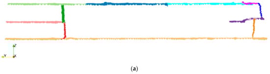
Figure 1. Example of the segmented trajectory of a multi-story building; (a) intermediate data, with the sub-trajectories of the top story having different average height or discontinuity in timestamp; (b) the trajectory after the final segmentation.

3.2. Room Identification by Analyzing the Trajectory Dataset Only

In this approach, the sub-trajectory of each story is analyzed independently as a spatiotemporal dataset to assign semantic labels describing the indoor spaces. The labels are rooms and doorways. The trajectory dataset is much smaller than the point cloud dataset in terms of the number of points. Therefore, the complexity of the analysis is reduced when processing the trajectory in the case of large buildings. Human trajectories have been used before as independent datasets to derive approximate floorplans. In our proposed method, the operator scanning behavior is interpreted to identify the spaces. The operator usually tends to slow down near transitional areas such as doorways and tight bends, to scan all the features properly, and to keep the connection to previously acquired areas, which is required by the simultaneous localization and mapping (SLAM) algorithms. Therefore, detecting the slowdowns along the trajectory can give an indication of the existence and location of doorways. Moreover, we can expect more trajectory points that form a loop near the doorways as the operator passes through the door when entering and leaving the room.

Figure 2 shows the pipeline for analyzing the trajectory dataset only. After segmenting the trajectory as described in Step 3.1, the trajectory of each story is processed individually. Similar to the trajectory-based clustering approaches [36,37], the scanning patterns are detected by joining changes in the movement direction with changes in movement speed to identify the rooms. In order to do this, the trajectory is first simplified. Then, the critical points that represent changes in speed and changes in movement direction are detected. After that, the rooms are identified and labeled by clustering the trajectory points according to the specified rules. Finally, the room labels are transferred to the point cloud using the timestamps in both datasets.

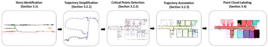
Figure 2. The pipeline for room identification by analyzing the trajectory only.

3.2.1. Trajectory Simplification

This step aims to remove the redundant trajectory points, and to keep fewer points without affecting the geometric trend of the trajectory. Furthermore, this process assists in bringing the trajectories from different scanners to the same geometric representation. The trajectory shape can vary from one scanning system to another, according to the scanner mechanism. For example, the laser scanner of the ZEB1 system is loaded on a spring mechanism. The shape of the scanner trajectory is irregular, as the scanner loosely oscillates about the spring. Other scanning systems such as ZEB-REVO or trolley-based systems have more regular moving patterns.

The radial distance-based algorithm described by Shi & Cheung is applied [38]. The algorithm considers the first point of the trajectory as a key point. It then iterates over the trajectory points, and it eliminates the succeeding points within a specified radius. After that, the first point outside that radius becomes a new key point. The algorithm stops when it reaches the last point of the trajectory. This algorithm has an advantage over down-sampling techniques, such as using voxels, as it respects the time order of the trajectory points besides the point spacing. Figure 3 shows an example of a sub-trajectory before and after the simplification process. The number of the trajectory points is reduced while maintaining the trend of the trajectory. The simplified trajectory acts as a base for detecting the critical trajectory points, as it has equally spaced points. Therefore, the line segments between each successive points are comparable along the simplified trajectory, which can be used to analyze movement characteristics such as speed, movement direction, and the length of the sub-trajectory [39].

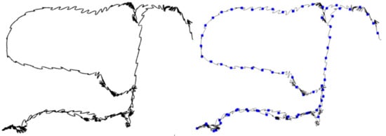
Figure 3. The trajectory (ZEB1) simplified using radial distance in blue dots (left) overlaid on the original trajectory (right).

3.2.2. Critical Points Detection

The simplification process focuses only on the geometric shape of the trajectory without considering its semantic meaning. Critical points are used to describe the important features and the transitions of the trajectory. For example, changes in movement direction can be described by fewer points, and the redundant points are removed. Therefore, the computation will be simpler than processing the full trajectory [40,41]. We distinguish between two different types of critical points:

Time-Critical points: The time-critical points indicate where there is a change in the movement speed along the trajectory. The time difference between each adjacent point is calculated and compared to a certain threshold. If the time difference exceeds a threshold of N seconds, the two points are marked as time-critical points.

Geometric-Critical points: The Douglas–Peucker algorithm [42] is used to detect the turning points along the trajectory. It is widely used to detect the critical points, as it preserves the direction trends using a perpendicular distance-based threshold [43].

Figure 4 shows the distribution of the critical points along a trajectory of one story. In total, the original trajectory contains 37,560 points, and it is simplified to 121 critical points. It is noticeable that there is a pattern of slowdowns near the doorways. However, the operator can change his movement speed at any place, depending on the environment. Therefore, the change in movement direction is combined with the change in speed in the next step to identify the rooms.

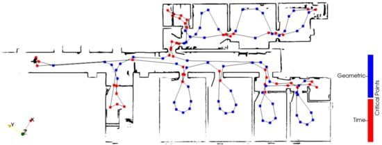
Figure 4. Example of critical points for a simplified trajectory.

3.2.3. Trajectory Annotation

In this step, additional labels representing rooms and doorways are added to the trajectory dataset. The critical points of the trajectory are used as an input for this step. Basically, the rooms are identified as the sub-trajectories that form a closed or semi-closed loop. The other unclassified trajectory parts are clustered together, based on their proximity to form another space. The doorways are assumed to be the connectors between the rooms.

Each two successive critical points form a line segment, while a sub-trajectory consists of one or more line segments. The algorithm iterates over a set of line segments that represent the trajectory that contains the critical points only.

Figure 5 shows the steps used to label the different rooms using the trajectory. The start point of a line segment is considered a key point. This key point is marked as being time-critical, which indicates that the operator slowed down, or that there is a change in the movement direction between two line segments. A nearest-neighbor search of the key point is applied to obtain all of the nearby critical points (checkpoints). A sub-trajectory containing all the critical points between the key point and checkpoint is constructed. Then, the following rules are applied to identify the sub-trajectory of a room:

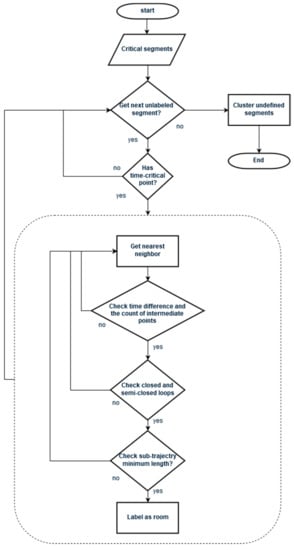
Figure 5. The steps for identifying the rooms based on the trajectory only.

• Size of the sub-trajectory: The sub-trajectory should be small enough to be within one space. The first criterion is the total time in seconds between the key point and the checkpoint, which indicates the duration that is spent to scan the space. It should not exceed a certain threshold. The second criterion limits the total number of the critical points between the key point and the checkpoint. It indicates the approximate length of the trajectory without the need to make the exact calculations.
• Self-Intersections: After that, the algorithm searches for self-intersections of the sub-trajectory. To detect semi-closed loops, the distances between the start and end points of the sub-trajectory should not exceed a certain distance, which is the target door width.

If the sub-trajectory passes the described checks, it is labeled as a room. The remaining unlabeled parts of the trajectory are clustered based on the Euclidian distance to be grouped into one or more space. The door positions are identified to be the connection points between two different rooms.

So far, the analysis is performed on the simplified trajectory. The original trajectory points are annotated using the timestamp intervals for each labeled room. The labels are transferred from the annotated trajectory to the corresponding story sub-cloud using the timestamp in both datasets.

3.3. Room Identification by Analyzing the Point Cloud Beside the Trajectory

In our second method, the point cloud dataset is processed with the help of the system trajectory. The experimental results of the previous method, which are discussed in Section 4.3, show that the scanning behavior of the operator has a great influence on the quality of the results. To override this influence, there is a need to process the point cloud in conjunction with the trajectory, as the point cloud represents the environment. Figure 6 shows the pipeline of the proposed method. The trajectory is used to limit the data to be analyzed to only the interesting spots of the point cloud, such as the possible doorway positions. It is used to detect the doors, which are the key elements for the space subdivision in our pipeline. The idea is to locate sub-clouds that are possible candidates for a door frame. Then, the nearby trajectory points between the doors are clustered and labeled as a room. Finally, the labels are transferred to the point cloud using the timestamp of the labeled trajectory.

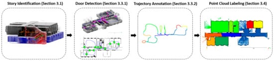
Figure 6. The pipeline for room identification by analyzing the point cloud beside the trajectory.

Door Detection

The trajectory dataset holds information about the topological structure of the indoor environment as the operator walks through different spaces during the scanning process. Doors are the key element for connecting the spaces, and the trajectory implicitly maps the location of the doors that are traversed by the operator, but the exact locations can be identified with the help of the point cloud. Consequently, the trajectory is used to identify the candidate door spots of the point cloud by extracting only the laser points which are near to the trajectory within a specific distance. Then, the candidate spots are segmented to detect planar patches that represent the walls surrounding the door frame. Finally, the trajectory is used again to verify the candidate door’s width and height, and the door position is labeled on the trajectory. The door height is validated after checking the door width as the distance between the top of the door, and the ceiling can be very small in the case of a railing door or the doors in a basement. Therefore, it is more reliable to check the door width first, and then to check for the door height. This method is used to detect opened, semi-opened, and closed doors (which were passed by the operator) through the following steps:

Input preprocessing: The sub-cloud of the story and its corresponding trajectory are the inputs for this method. The trajectory is simplified with a small tolerance to reduce the number of the trajectory points, and to optimize the computations. A horizontal slice of the point cloud is used in this algorithm. The slice is taken at the trajectory’s average height level ±0.25–0.30 m. This trajectory level is expected to have a low level of clutter, and also, the slice height is enough to detect the planar patches.

Door spots identification: A radius search between every trajectory point and sub-cloud slice is applied to detect the objects nearby the trajectory. These objects can be the walls that are near the trajectory that represent the door boundary. To ensure that the points are dense enough to represent a wall, the radius search is constrained with a minimum number of neighboring laser points. If that number exceeds a threshold (e.g., 500 points), the trajectory point and its neighboring laser points are marked as a possible door spot.

After identifying all of the door candidates, the trajectory points are clustered based on the Euclidean distance. Each cluster of the trajectory points represents one or more door candidates located nearby. The corresponding sub-cloud that represents the door spots is saved beside its trajectory. Figure 7 shows an overview of the results; the candidate trajectory points are colored in red, and their corresponding point clouds are colored in purple. Each sub-trajectory with its sub-cloud is processed individually in the next step.

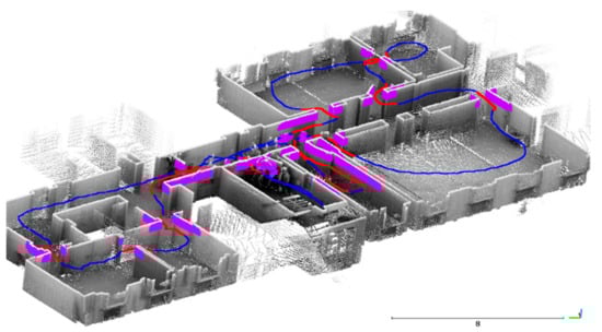
Figure 7. Candidate trajectory points (red) over the full trajectory (blue). The nearby laser points of the slice that represent the door spots (purple).

Each sub-cloud is analyzed to detect the wall candidates that surround the opening. The door plane is assumed to be part of a wall surface in the case of a closed door, as the trajectory will intersect with that plane and a gap in an existing wall segment, in the case of opened doors. First, the sub-cloud is down-sampled to voxels of a size of 0.05 m, and segmented using a surface growing method [44]. Then, the segments are processed to keep only the ones that are parallel to the z-axis with a tolerance of 10 degrees. After that, the semi-opened door leaves are eliminated by keeping only the surfaces that are parallel or perpendicular to the dominant wall direction of the sub-cloud within a threshold of 10 degrees.

Door width validation: So far, the candidate walls and their nearby trajectory are selected. In this step, the door width is validated using proximity rules between the trajectory and the detected walls. The idea is to label the trajectory points that represent a door position. Firstly, the trajectory is simplified a with 0.01 m tolerance to improve the computation speed. Then, a nearest neighbor search between every trajectory point and the wall segments are used to obtain the nearby walls within a specified distance (e.g., 0.80 m). If the distance between a trajectory point and a wall segment is less than 0.1 m, it is flagged as a door candidate, as it can represent a closed door. In the case of an opened door, the width of the gap between every two wall candidates is verified. The trajectory point is marked as a door candidate if it is collinear with the two points that represent the nearest neighbors from the walls with some tolerance (e.g., 10 degrees). In addition, the trajectory point should be in the center between those two points. The length of the line constructed between the two wall points should be below the door-width threshold (e.g., 1.0 m). If the trajectory point satisfies these conditions, it is validated for the door height, as the point can be misidentified if it is passing through narrow pathways, or between high furniture objects such as bookshelves. The door width validation step is described in Algorithm 1.

Door height validation: In this check, the door height is validated using the voxel space of the full story point cloud. A voxel size of 0.05 m is used. The occupied voxels above and below each trajectory candidate are queried. For the voxels below the trajectory, the lowest voxel is assumed to be at floor level. Then, the net height between the floor level and the voxels above the trajectory point is calculated. The trajectory point is identified as the final door point if there are occupied voxels at a height within a threshold (e.g., between 1.80 m and 2.20 m). Finally, the nearby door points are clustered together with a clustering tolerance of 0.50 m to identify the trajectory points that belong to each door. Then, the points are labeled in the full trajectory using the timestamp. The door height validation step is described in Algorithm 2.

After identifying the doors, the nearby sub-trajectories between the doors are clustered together and labeled as a room. Also, the clustering step uses Euclidean distance clustering to group the nearby trajectories into one space in the case of a corridor that connects multiple rooms. Figure 8 shows the annotated trajectory of a two-story building.

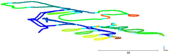
Figure 8. Annotated trajectory based on the identified doors. The doors are colored in cyan, and each annotated space has a different color.

Algorithm 1. Pseudo-code for door width validation.

1 INPUT

2 door_spot_lst //door spot sub-cloud and its corresponding trajectory points

3 OUTPUT

4 door_sub_trajectory //candidates to be validated for door height

5 METHOD:

6 SET searchRadius to 1.0 meters //to get planes nearby trajectory points

7 FOREACH (door_sub_trajectory and door_sub_cloud IN door_spot_lst)

8  //1. apply region growing to detect planes

9  segmented_cloud = Segment_point_cloud(door_sub_cloud)

10  //2. get planer surfaces which represent the door boundary

11  plane_lst = GetPlanerSurfaces(segmented_cloud);

12  FOREACH trajectory_point IN door_sub_trajectory

13   trajectory_point is not a door candidate // set initial state

14   //3. Get the surfaces near the trajectory point

15   np= GetNearestPlanes(trajectory_point, plane_lst, searchRadius)

16   FOREACH plane IN np

17    //4. Construct line from the point to every nearby surface

18    ls= CreateLineSegmentFromTrajectoryPointToNearstPointOnThe

19    Plane(trajectory_point,p)

20    add ls and plane to pt_plane_line_lst

21   ENDFOR

22   FOR i from 0 to pt_plane_line_lst.size() DO

23    indexSegment = pt_plane_line_lst [i]

24    //5. Closed door case

25    IF (indexSegment.Length is less than 0.10 meters)

26     trajectory_point is a door candidate

27     CONTINUE

28    ENDIF

29    //6. If the trajectory point between two planes and the distance

30    //between the two planes are within the door width threshold, it is

31    //marked as door candidate

32    FOR j from i + 1 to pt_plane_line_lst.size() DO

33     followingSegment = pt_plane_line_lst [j]

34    // both segments share the start point which is the trajectory point

35    //the end point is the nearest point on the plane

36     IF (indexSegment and followingSegment are near-collinear)

37      doorWidth = GetDistanceBetweenTwoPoints(indexSeg-

38      ment.EndPoint(), followingSegment.EndPoint())

39      //Check door width

40      IF (doorWidth less than or equal to target door width)

41       // update the new state

42       trajectory_point is a door candidate

43      ENDIF

44     ENDIF

45    ENDFOR

46   ENDFOR

47  ENDFOR

48 ENDFOR

49 RETURN door_sub_trajectory

50 ENDMETHOD

Algorithm 2. Pseudo-code for door height validation.

1 INPUT

2 alidation

3 pc_voxels //point cloud in voxel representation

4 OUTPUT

5 final_door_point_list //final trajectory door points

6 METHOD:

7 FOREACH door_point IN door_point_list

8  IF (door_point is a door candidate)

9  // get occupied voxels above and below the trajectory candidate

10   top_voxel_list = GetOccupiedVoxelsAboveThePoint(pc_voxels)

11   ground_voxel_list = GetOccupiedVoxelsBelowThePoint(pc_voxels)

12   IF (No Voxels Up or Below)

13    door_point is not a door candidate

14    CONTINUE

15   ENDIF

16   //get ground point

17   ground_voxel = GetLowestOccupiedVoxel(ground_voxel_list)

18   door_point is not a door candidate //reset the point state

19   FOREACH top_voxel IN top_voxel_list

20    door_height_tmp = top_voxel.z - ground_voxel.z

21    IF (door_height_tmp within door height range)

22     door_point is a final door point

23     add door_point to final_door_point_list

24     BREAK

25    ENDIF

26   ENDFOR

27  ENDIF

28 ENDFOR

29 RETURN final_door_point_list

30 ENDMETHOD

3.4. Point Cloud Labeling and Post Processing

In the previous steps, the sub-cloud of the story is initially labeled with the room information, based on the annotated trajectory. The labels are transferred, using the timestamps in both datasets. However, the subdivided spaces contain mixed labels within the space, as shown in Figure 9a. This can be expected if spaces are bounded by glass walls, or if part of the space is scanned from another space through an open door. A majority filter is applied to the story sub-cloud to refine the labeling results. The points in one space should have the same label with the assumption of having vertical walls. Therefore, the filter is applied to a projection of the point cloud into the 2D plane. First, a quadtree with a 0.05 m cell size is constructed from the projected points. Then, each occupied cell is assigned to the label that represents the majority of the points inside. Next, the trajectory is involved in the filtering by assigning the cells that are near to the trajectory with the same label as the trajectory points. The trajectory helps to enhance the labeling near the doors, as there are many mixed labels. After that, another iteration of the majority filter is applied to consider the direct neighbors of the labeled cells to eliminate the misclassified small spots. Finally, the labels are transferred back to the 3D point cloud. Figure 9b shows the result after applying the majority filter for one of the stories, and Figure 10 shows its 3D view.

Figure 9. Example for a top view of the labeled point cloud; (a) only by using a timestamp, (b) after applying the majority filter. The ceiling is removed for visualization purposes.

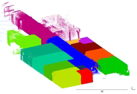
Figure 10. 3D view for a story after subdividing it into rooms.

4. Experiments and Results

4.1. Datasets

Four mobile laser scanner datasets with a total of seven stories are used to evaluate the proposed approaches. They all provide the point cloud beside the scanner trajectory, and the two datasets are related by timestamps. Table 1 shows the specifications of the datasets and the scanning systems used for data acquisition. Figure 11 shows an overview of the datasets. The first three datasets were captured in one of the buildings of the Technische Universität Braunschweig, Germany, with different scanning systems. Datasets 1 and 2 represent only one story while dataset 3 has two stories connected by a staircase. Datasets 2 and 3 are part of the ISPRS indoor benchmark datasets [45]. Dataset 4 was captured in the building of the fire brigade in Berkel en Rodenrijs, The Netherlands with the ZEB1 scanner. It consists of three stories connected by staircases. The dataset has a high level of clutter, due to the presence of the furniture. Also, it contains many glass walls and windows, which makes it challenging during the semantic labeling process. The size of the trajectory dataset is smaller than the point cloud dataset in terms of the total number of points.

Table 1. Specifications of the point cloud datasets.

Dataset	Number of Stories	Number of Laser Points	Number of Trajectory Points	Level of Clutter	Scanning System
Dataset 1	1	37.3 × 106	22.4 × 103	low	ITC Backpack [46]
Dataset 2	1	33 × 106	89.3 × 103	low	Viametris iMS3D
Dataset 3	2	21.6 × 106	65.9 × 103	low	ZEB-REVO
Dataset 4	3	79.1 × 106	219.3 × 103	high	ZEB1

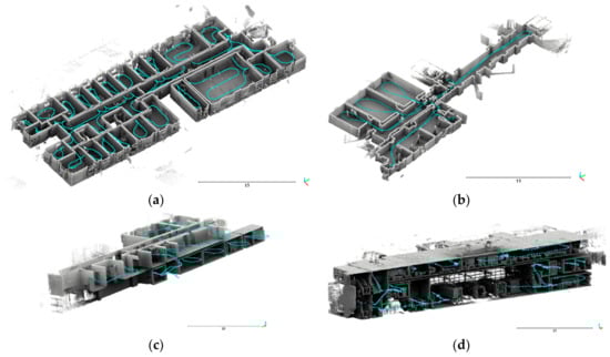
Figure 11. Overview of the datasets; (a) dataset 1; (b) dataset 2; (c) dataset 3; (d) dataset 4. The scanner trajectory is colored in cyan. The ceiling and parts of the point cloud are removed for visualization purposes.

The proposed approach was developed using C++ and the Point Cloud Library (PCL). The trajectory is stored in a SQLite database where all the labels are added to the same file. The experiments were performed using a laptop computer with Intel Core i7 (2.6 GHz, 16.0 GB of RAM).

4.2. Story and Staircase Identification

Datasets 3 and 4 are used to test the proposed method for identifying the stories and the staircases, as they represent multi-story buildings. Figure 12 shows the results of dataset 3. Two stories are identified besides the staircase. There is an overlap between the identified spaces, as shown in Figure 12b,c as the separation is done by using the timestamp of the point cloud and the trajectory datasets. A height histogram of the point cloud can be applied to detect the floor and ceiling levels, to eliminate any extra laser points. Figure 13 shows the results of dataset 4. The ground story of the dataset has different ceiling heights, and it was separated from the other spaces, as shown in Figure 13b. More overlap between the spaces can be noticed in Figure 13c, as the spaces have glass walls.

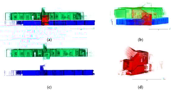
Figure 12. Overview of story identification for dataset 3; (a) the stories and staircases are labeled in different colors; (b) cross-section in the dataset; (c) the two identified stories; (d) the staircase.

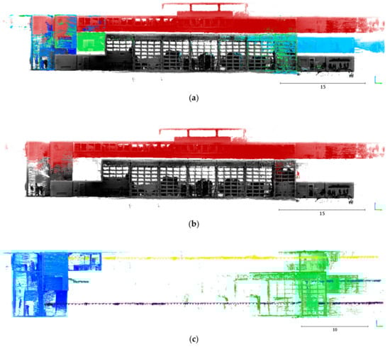
Figure 13. Overview of story separation for dataset 4; (a) the stories and staircases are labeled in different colors; (b) the top and ground story only; (c) the staircases with the segmented trajectory.

Table 2 shows the parameters used during the story identification. The choice of the parameters is determined by experiments, as the processing time is a few seconds, and the parameters can be modified interactively by the user. The choice of the sliding window width (w) is 400 points, and this is equivalent to 4 s for a 100 Hz scanning rate for a scanner such as ZEB-REVO. The proper selection of the parameter is essential to properly estimate the mean height, especially in the case of the ZEB1 trajectory, which has an irregular shape. During the merging phase, a parameter of the second neighbor height difference (h₂) is used to detect any gradual changes in height between the windows. The merging threshold for the adjacent segments can vary, depending on the environment. P_min is responsible for distinguishing horizontal segments from staircase segments. It should be larger than w, as the segment will be merged with its neighbor if both of them are below that threshold. In the final step of the algorithm, h₃ can be increased if the place has different floor levels, but in the same story to include all the trajectory points into a one-story segment.

Table 2. Parameters used for story identification.

Parameter	Value
Sliding window width w	400 points
The first Neighbor height difference h1	0.20 m
The second Neighbor height difference h2	0.30 m
Minimum points per segment Pmin	1000 points
Merging adjacent segments height difference h3	0.40 m

4.3. Room Identification by Analyzing the Trajectory Dataset Only

The trajectory dataset is analyzed as an independent source of information to identify the rooms. This dataset is very small comparing to the corresponding point cloud, but this method is highly influenced by the operator behavior. Figure 14 shows the experiments on dataset 1 and the same story from dataset 3. The rooms that are captured by using the closed loop pattern are identified as shown in Figure 14a, while they are not identified when the operator uses a different strategy for data capture, as shown in Figure 14b. Also, the method has a limitation in that it identifies the rooms with more than one door, as the current method only detects the movement in loops. The scanning pattern for a room with more than one door can be performed in many ways. Therefore, there is no pattern to detect this behavior, unless the doors are identified first, which requires the help of the point cloud. The trajectory-based method can be applied when the operator follows predefined scanning rules. Also, analyzing the trajectory data can help to develop the best practice for scanning complex buildings by analyzing the scanning behavior.

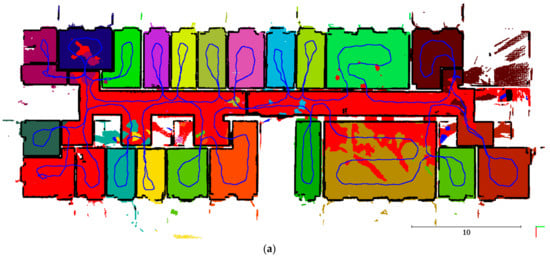
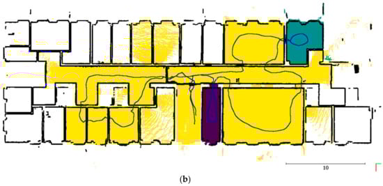
Figure 14. The result of room identification by analyzing the trajectory dataset only; (a) a single story of Dataset 1, (b) the similar story in Dataset 3.

Table 3 shows the parameters used for this method. The trajectory that represents a room is described by the maximum size of the space, which is described by t_max and p_max. The minimum size of the space is described by l_min, and it is mainly used to eliminate the small bends and loops in the trajectory. For example, the smallest space could be a restroom that takes 2–5 s to scan; hence, the size of the trajectory should not be more than 2–4 steps, which is equivalent to 3.20 m when using 0.80 m as the trajectory simplification tolerance. The value of t_max is affected by the operator scanning behavior, as it indicates the time that is spent inside the space. Also, the operator behavior is affected by the scanning system. For example, the value of t_max is 45 s for datasets 1–3, while it is increased to be 120 s in the case of the ZEB1 system for dataset 4. Also, using larger values can result in multiple adjacent spaces having one label.

Table 3. Parameters used for the trajectory analysis.

Parameter	Value
Nearest neighbor search tolerance r	1.0 m
Maximum scanning time within a space tmax	45 s
Maximum critical points within a space pmax	20 points
Minimum trajectory length within a space lmin	3.20 m

4.4. Room Identification by Analyzing the Point Cloud Beside the Trajectory

In this approach, doors are considered to be the essential element that is used to subdivide the spaces. The trajectory is used to identify the spots where possible doors are located. Table 4 shows the parameters for identifying the door spots. The trajectory is simplified by a tolerance (r = 0.20 m), as every trajectory point is used to obtain nearby laser points. In this case, the simplification threshold is used to eliminate the redundant points and to optimize the performance. The two main parameters in this step are the search tolerance (dn) and the minimum number of neighboring points (p_min). The first parameter (dn) is responsible for extracting the laser points near the trajectory. During the experiments, the value varied from 0.80 m to 1.20 m. Figure 15 shows an example of changing the dn value from 0.80 m to 1.10 m. Increasing the value is used to obtain enough points for segmenting the openings’ boundaries. The initial value can be equal to the target door width to obtain enough laser points on both sides. However, if the value is more than the optimum, the generated door spot can contain multiple door candidates that will increase the processing time. Also, it may affect the calculation of the dominant wall direction. The minimum neighboring points (p_min) has a wider range of between 100 points to 5000 points. The value of p_min is adjusted according to the level of clutter and the point density of the point cloud dataset. It is increased to (p_min = 5000 points) in the case of dataset 4, as it contains a high level of clutter and false walls that are reflected from the glass surfaces in the building. This parameter helps to eliminate the temporary objects and the reflected walls by only keeping the dense elements. Changing the value of p_min does not affect the segmentation results in the following steps, as the sub-cloud is down-sampled before the segmentation.

Table 4. Parameters used to identify the door spots.

Parameter	Value
Trajectory simplification tolerance r	0.20 m
Neighbors search tolerance dn	0.80 to 1.20 m
Minimum neighboring points pmin	100 to 5000 points

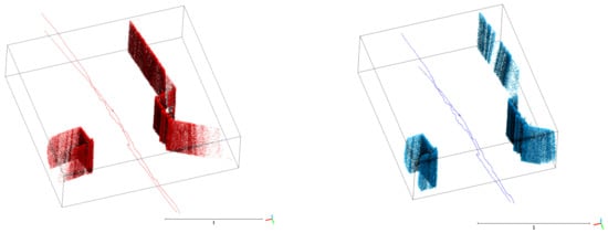
Figure 15. Example of changing the search tolerance value to identify the door spots. dn = 1.10 m (red) and dn = 0.80 m (blue). The red sub-cloud has more laser points, which gives better segmentation results.

Table 5 shows the parameters used for door detection. They validate the width and the height of the candidate door. The door width d_max can be changed to fit the target door width. The chosen value is d_max = 1.10 m, which covers all of the doors that are passed by the operator in the datasets.

Table 5. The parameters used to detect the doors.

Parameter	Value
Search radius for door boundary r	0.80 m
Closed door distance threshold dc	0.10 m
Maximum door width dmax	1.10 m
Minimum door width dmin	0.50 m
Door height threshold hd	1.80 to 2.20 m
Door cluster tolerance rd	0.50 m
Trajectory cluster tolerance tc	0.30 m

Another limitation for the door detection method is by using a range threshold hd to determine the door height. This can be a limitation in environments that have doors that vary in their heights, and the ceiling level falls to within the door height range, hd. This case can result in false doors. Also, using the threshold dc to identify the closed doors as an intersection between the trajectory and the point cloud can result in false doors when the trajectory is very near to the wall candidates, as shown in Figure 16. These false doors are eliminated by using the trajectory cluster tolerance tc.

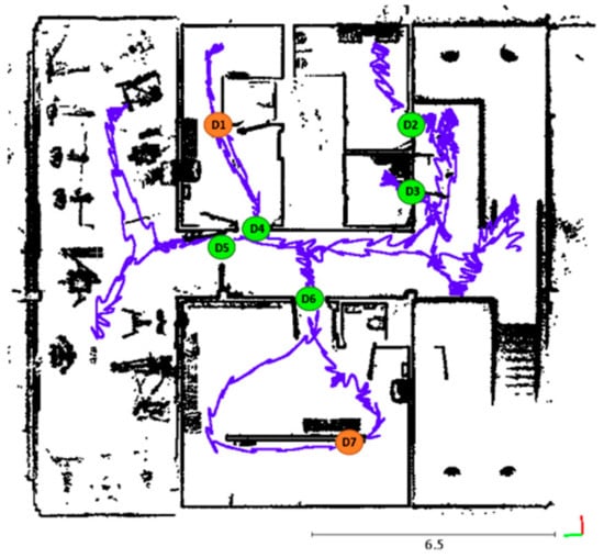
Figure 16. Example of false doors shown in orange, as the trajectory is very near to the point cloud. The green dots are the correct doors.

The trajectory cluster tolerance (tc = 0.30 m) is responsible for clustering the trajectory points between the doorways. All of the nearby trajectory points within that threshold are labeled as one room. One of the limitations of using this parameter is the over-segmentation of the narrow paths, such as in the case of corridors if they are not covered with enough trajectory points, as shown in Figure 17 and Figure 18. This case appears with rooms that have more than one door, and when the trajectory points between these two doors are not close enough to be clustered as one space.

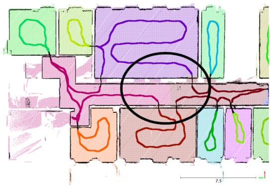
Figure 17. Example of over-segmentation (black circle) in identifying the rooms caused by using the method clustering of the nearby trajectory points.

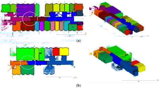
Figure 18. Room identification results; (a) dataset 1, (b) a similar story in dataset 3. The white circle shows an over-segmentation problem illustrated in Figure 17.

Table 6 and Table 7 summarize the results of door detection and room identification methods, respectively. Table 6 shows the total number of doors within each story, the number of correctly detected doors, and the accuracy result. Table 7 shows the same statistics for the rooms. The figures below show the final results of the room identification after applying the majority filter. Figure 18 shows an overview of the results of the same story in dataset 1 and dataset 3 (story 3-1). The yellow room in Figure 18b was the result of removing a wall between the data acquisitions. Both stories have a clear separation of the rooms. However, they also have a problem of over-segmentation in the corridor part. Both stories have a misidentified room, although all of the doors are detected correctly. The over-segmentation problem can be recovered by analyzing the intersection between every two spaces to validate the existence of the separators (e.g., common walls).

Table 6. Summary results for door detection. Number of detected doors shows the correctly detected ones.

Dataset (-story)	No. of Doors	No. of Detected Doors	Precision	Recall
Dataset 1	28	28	1	1
Dataset 2	10	10	1	1
Dataset 3-1	11	11	1	1
Dataset 3-2	14	14	1	1
Dataset 4-1	8	8	1	1
Dataset 4-2	5	5	0.71	1
Dataset 4-2	1	1	1	1
Dataset 4-3	17	16	0.94	0.94

Table 7. Summary results for room identification. Number of detected rooms shows the correctly detected ones.

Dataset (-story)	No. of Rooms	No. of Detected Rooms	Precision	Recall
Dataset 1	25	25	0.96	1
Dataset 2	10	10	1	1
Dataset 3-1	9	9	0.9	1
Dataset 3-2	15	15	1	1
Dataset 4-1	8	8	1	1
Dataset 4-2	8	8	1	1
Dataset 4-2	2	2	1	1
Dataset 4-3	16	-	-	-

Figure 19 shows the results of dataset 2 and the same story in dataset 3 (story 3-1). All of the rooms and the doors are identified correctly in both datasets. The points outside the building layout have the same label as the space from which they were captured. However, the points have the same labels as the nearest room after applying the majority filter. These points can be identified and labeled with different labels by analyzing the individual rooms and applying, for example, ray tracing, but this is out of the scope of this research.

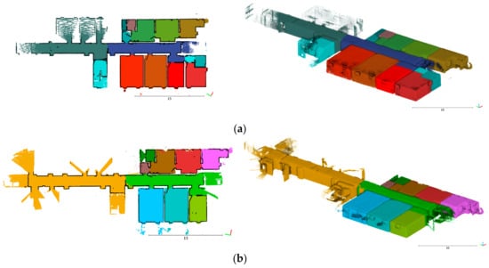
Figure 19. Room identification results; (a) dataset 2, (b) a similar story in dataset 3.

Figure 20 shows the results of dataset 4, which represents a three-story building. The building has many glass walls that cause the scanning of a room from outside its space. This poses the challenge of overlap between different spaces. Figure 20b (story 4-3) clearly showed one limitation of the proposed method where there is a high level of over-segmentation of the detected spaces. The over-segmentation appears due to the high level of clutter in some rooms, as some parts inside the rooms were not scanned properly. The initial labels of the laser points are transferred from the annotated trajectory using the timestamp in both datasets. Therefore, the glass walls of the rooms in combination with the labeled rooms caused the majority filter to fail, as the majority of the points inside the rooms were scanned from outside. In total, 16 out of 17 doors were detected for this story, as well as one false door, but the glass walls had more influence on the results. Also, the same problem of the glass walls appears in Figure 20a (story 4-1) as it has fewer glass walls. All of the rooms and doors are identified correctly. The intermediate story (story 4-2) has two false doors, but these doors are eliminated during the door detection process. One limitation for our approach is that the labeling process does bit exclude artifacts outside the building layout, as it is based on the timestamp. Moreover, the detected doors are only the ones that are traversed by the operator during the scanning. As a result, the rooms that are partially scanned from outside cannot be identified independently.

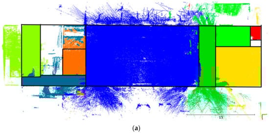
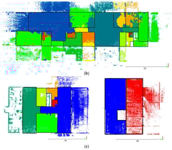
Figure 20. Room identification results for dataset 4; (a) The top story (4-1), (b) the ground story (4-3), (c) the intermediate stories (4-2).

5. Conclusions

In this research, IMLS data is enriched with semantic labels of the indoor spaces by using the trajectory of the scanner as a source of information. The first label carries information about the stories and the staircases, and the second label about the rooms and doorways. The trajectory dataset is used to split and process small chunks of the point cloud that can improve the processing performance for the large datasets. The trajectory is used to identify the stories and the staircases. In addition, it is analyzed in conjunction with the point cloud to identify the doorways and the rooms. The output of this research is labeled IMLS data, which can be used in a domain-specific application, and it can be divided into smaller chunks based on these labels (e.g., room-by-room processing). The experiments on four real-world datasets showed the effectiveness and the flexibility of the proposed method regarding the scanning behavior of the operator and the scanning system. Only a few rooms are not detected, due to over-segmentation. However, the method showed a limitation in identifying the spaces where there are glass walls. Also, this approach is limited to the IMLS data, as it depends on the trajectory dataset. Reconstructing the interior models and labeling the point cloud in near real-time are possible avenues of future work.

References

- Tang, P.; Huber, D.; Akinci, B.; Lipman, R.; Lytle, A. Automatic reconstruction of as-built building information models from laser-scanned point clouds: A review of related techniques. Autom. Constr. 2010, 19, 829–843. [Google Scholar] [CrossRef]
- Okorn, B.; Xiong, X.; Akinci, B.; Huber, D. Toward Automated Modeling of Floor Plans. In Proceedings of the Symposium on 3D Data Processing, Visualization and Transmission, Paris, France, 17–20 May 2010; Volume 2. [Google Scholar]
- Xiong, X.; Adan, A.; Akinci, B.; Huber, D. Automatic creation of semantically rich 3D building models from laser scanner data. Autom. Constr. 2013, 31, 325–337. [Google Scholar] [CrossRef]
- Mura, C.; Mattausch, O.; Jaspe Villanueva, A.; Gobbetti, E.; Pajarola, R. Automatic Room Detection and Reconstruction in Cluttered Indoor Environments with Complex Room Layouts. Comput. Graph. 2014, 44, 20–32. [Google Scholar] [CrossRef]
- Mozos, O.M.; Stachniss, C.; Burgard, W. Supervised Learning of Places from Range Data using AdaBoost. In Proceedings of the 2005 IEEE International Conference on Robotics and Automation, Barcelona, Spain, 18–22 April 2005; pp. 1730–1735. [Google Scholar]
- Pronobis, A.; Martínez Mozos, O.; Caputo, B.; Jensfelt, P. Multi-modal semantic place classification. Int. J. Rob. Res. 2010, 29, 298–320. [Google Scholar] [CrossRef]
- Díaz-Vilariño, L.; Boguslawski, P.; Khoshelham, K.; Lorenzo, H.; Mahdjoubi, L. Indoor navigation from point clouds: 3D modelling and Obstacle Detection. Int. Arch. Photogramm. Remote Sens. Spat. Inf. Sci. ISPRS Arch. 2016, 41, 275–281. [Google Scholar] [CrossRef]
- Lehtola, V.; Kaartinen, H.; Nüchter, A.; Kaijaluoto, R.; Kukko, A.; Litkey, P.; Honkavaara, E.; Rosnell, T.; Vaaja, M.; Virtanen, J.-P.; et al. Comparison of the Selected State-Of-The-Art 3D Indoor Scanning and Point Cloud Generation Methods. Remote Sens. 2017, 9, 796. [Google Scholar] [CrossRef]
- Sirmacek, B.; Shen, Y.; Lindenbergh, R.; Zlatanova, S.; Diakite, A. Comparison of Zeb1 and Leica C10 Indoor Laser Scanning Point Clouds. ISPRS Ann. Photogramm. Remote Sens. Spat. Inf. Sci. 2016, III-1, 143–149. [Google Scholar] [CrossRef]
- Contreras, L.; Mayol-Cuevas, W. Trajectory-driven point cloud compression techniques for visual SLAM. In Proceedings of the 2015 IEEE/RSJ International Conference on Intelligent Robots and Systems (IROS), Hamburg, Germany, 28 September–2 October 2015; pp. 133–140. [Google Scholar] [CrossRef]
- Xie, L.; Wang, R. Automatic Indoor Building Reconstruction from Mobile Laser Scanning Data. Int. Arch. Photogramm. Remote Sens. Spat. Inf. Sci. 2017, XLII-2/W7, 417–422. [Google Scholar] [CrossRef]
- Díaz-Vilariño, L.; Verbree, E.; Zlatanova, S.; Diakité, A. Indoor Modelling from Slam-Based Laser Scanner: Door Detection to Envelope Reconstruction. ISPRS Int. Arch. Photogramm. Remote Sens. Spat. Inf. Sci. 2017, XLII-2/W7, 345–352. [Google Scholar] [CrossRef]
- Turner, E.; Zakhor, A. Multistory Floor Plan Generation and Room Labeling of Building Interiors from Laser Range Data; Springer: Cham, Switzerland, 2015; pp. 29–44. [Google Scholar]
- Ochmann, S.; Vock, R.; Wessel, R.; Klein, R. Automatic Reconstruction of Parametric Building Models from Indoor Point Clouds. Comput. Graph. 2016, 54, 94–103. [Google Scholar] [CrossRef]
- Nikoohemat, S.; Peter, M.; Oude Elberink, S.; Vosselman, G. Exploiting Indoor Mobile Laser Scanner Trajectories for Semantic Interpretation of Point Clouds. ISPRS Ann. Photogramm. Remote Sens. Spat. Inf. Sci. 2017, IV-2/W4, 355–362. [Google Scholar] [CrossRef]
- Mura, C.; Mattausch, O.; Pajarola, R. Piecewise-planar Reconstruction of Multi-room Interiors with Arbitrary Wall Arrangements. Comput. Graph. Forum 2016, 35, 179–188. [Google Scholar] [CrossRef]
- Mozos, Ó.M. Semantic Labeling of Places with Mobile Robots; Springer Tracts in Advanced Robotics; Springer: Berlin/Heidelberg, Germany, 2010; Volume 61, ISBN 978-3-642-11209-6. [Google Scholar]
- Zheng, Y.; Peter, M.; Zhong, R.; Oude Elberink, S.; Zhou, Q. Space Subdivision in Indoor Mobile Laser Scanning Point Clouds Based on Scanline Analysis. Sensors 2018, 18, 1838. [Google Scholar] [CrossRef] [PubMed]
- Jung, J.; Stachniss, C.; Kim, C. Automatic Room Segmentation of 3D Laser Data Using Morphological Processing. ISPRS Int. J. Geo-Inf. 2017, 6, 206. [Google Scholar] [CrossRef]
- Ambrus, R.; Claici, S.; Wendt, A. Automatic Room Segmentation from Unstructured 3-D Data of Indoor Environments. IEEE Robot. Autom. Lett. 2017, 2, 749–756. [Google Scholar] [CrossRef]
- Bormann, R.; Jordan, F.; Li, W.; Hampp, J.; Hägele, M. Room segmentation: Survey, implementation, and analysis. In Proceedings of the IEEE International Conference on Robotics and Automation, Stockholm, Sweden, 16–21 May 2016; pp. 1019–1026. [Google Scholar]
- Shi, L.; Kodagoda, S.; Dissanayake, G. Laser range data based semantic labeling of places. In Proceedings of the 2010 IEEE/RSJ International Conference on Intelligent Robots and Systems (IROS), Taipei, Taiwan, 18–22 October 2010; pp. 5941–5946. [Google Scholar]
- Grzonka, S.; Karwath, A.; Dijoux, F.; Burgard, W. Activity-based Estimation of Human Trajectories. IEEE Trans. Robot. 2012, 28, 234–245. [Google Scholar] [CrossRef]
- Alzantot, M.; Youssef, M. CrowdInside: Automatic Construction of Indoor Floorplans. In Proceedings of the 20th International Conference on Advances in Geographic Information Systems—SIGSPATIAL’12, Redondo Beach, CA, USA, 6–9 November 2012; ACM Press: New York, New York, USA, 2012; p. 99. [Google Scholar]
- Grzonka, S.; Dijoux, F.; Karwath, A.; Burgard, W. Mapping indoor environments based on human activity. In Proceedings of the 2010 IEEE International Conference on Robotics and Automation, Anchorage, AK, USA, 3–7 May 2010; pp. 476–481. [Google Scholar]
- Fichtner, F.W.; Diakité, A.A.; Zlatanova, S.; Voûte, R. Semantic enrichment of octree structured point clouds for multi-story 3D pathfinding. Trans. GIS 2018, 22, 233–248. [Google Scholar] [CrossRef]
- Staats, B.R.; Diakité, A.A.; Voûte, R.L.; Zlatanova, S. Automatic Generation of Indoor Navigable Space Using a Point Cloud and Its Scanner Trajectory. ISPRS Ann. Photogramm. Remote Sens. Spat. Inf. Sci. 2017, IV-2/W4, 393–400. [Google Scholar] [CrossRef]
- Friedman, S.; Pasula, H.; Fox, D. Voronoi Random Fields: Extracting the Topological Structure of Indoor Environments via Place Labeling. In Proceedings of the 20th International Joint Conference on Artifical Intelligence (IJCAI’07), Kingston, ON, Canada, 13–17 August 2007; Morgan Kaufmann Publishers Inc.: San Francisco, CA, USA, 2007; pp. 2109–2114. [Google Scholar]
- Bobkov, D.; Kiechle, M.; Hilsenbeck, S.; Steinbach, E. Room Segmentation in 3D Point Clouds Using Anisotropic Potential Fields. In Proceedings of the 2017 IEEE International Conference on Multimedia and Expo (ICME), Hong Kong, China, 10–14 July 2017; pp. 727–732. [Google Scholar]
- McCormac, J.; Handa, A.; Davison, A.; Leutenegger, S. SemanticFusion: Dense 3D Semantic Mapping with Convolutional Neural Networks. In Proceedings of the 2017 IEEE International Conference on Robotics and Automation (ICRA), Singapore, 29 May–3 June 2017. [Google Scholar] [CrossRef]
- Bosse, M.; Zlot, R.; Flick, P. Zebedee: Design of a Spring-Mounted 3-D Range Sensor with Application to Mobile Mapping. IEEE Trans. Robot. 2012, 28, 1104–1119. [Google Scholar] [CrossRef]
- Balado, J.; Díaz-Vilariño, L.; Arias, P.; Soilán, M. Automatic building accessibility diagnosis from point clouds. Autom. Constr. 2017, 82, 103–111. [Google Scholar] [CrossRef]
- Oesau, S.; Lafarge, F.; Alliez, P. Indoor scene reconstruction using feature sensitive primitive extraction and graph-cut. ISPRS J. Photogramm. Remote Sens. 2014, 90, 68–82. [Google Scholar] [CrossRef]
- Khoshelham, K.; Díaz-Vilariño, L. 3D Modelling of Interior Spaces: Learning the Language of Indoor Architecture. ISPRS Int. Arch. Photogramm. Remote Sens. Spat. Inf. Sci. 2014, XL-5, 321–326. [Google Scholar] [CrossRef]
- Turner, E.; Zakhor, A. Watertight As-Built Architectural Floor Plans Generated from Laser Range Data. In Proceedings of the 2012 Second International Conference on 3D Imaging, Modeling, Processing, Visualization & Transmission, Zurich, Switzerland, 13–15 October 2012; pp. 316–323. [Google Scholar]
- Rocha, J.A.M.R.; Times, V.C.; Oliveira, G.; Alvares, L.O.; Bogorny, V. DB-SMoT: A Direction-Based Spatio-Temporal Clustering Method. In Proceedings of the 2010 5th IEEE International Conference Intelligent Systems, London, UK, 7–9 July 2010; pp. 114–119. [Google Scholar]
- Zhao, X.-L.; Xu, W.-X. A Clustering-Based Approach for Discovering Interesting Places in a Single Trajectory. In Proceedings of the 2009 Second International Conference on Intelligent Computation Technology and Automation, Changsha, China, 10–11 October 2009; pp. 429–432. [Google Scholar]
- Shi, W.; Cheung, C. Performance Evaluation of Line Simplification Algorithms for Vector Generalization. Cartogr. J. 2006, 43, 27–44. [Google Scholar] [CrossRef]
- Dodge, S.; Weibel, R.; Forootan, E. Revealing the physics of movement: Comparing the similarity of movement characteristics of different types of moving objects. Comput. Environ. Urban Syst. 2009, 33, 419–434. [Google Scholar] [CrossRef]
- Jin, P.; Cui, T.; Wang, Q.; Jensen, C.S. Effective Similarity Search on Indoor Moving-Object Trajectories; Springer: Cham, Switzerland, 2016; pp. 181–197. [Google Scholar]
- Buchin, M.; Driemel, A.; Van Kreveld, M.; Sacristan, V. Segmenting Trajectories: A Framework and Algorithms Using Spatiotemporal Criteria. J. Spat. Inf. Sci. 2011. [Google Scholar] [CrossRef]
- Douglas, D.H.; Peucker, T.K. Algorithms for The Reduction of the Number of Points Required to Represent A Digitized Line or Its Caricature. Cartogr. Int. J. Geogr. Inf. Geovis. 1973, 10, 112–122. [Google Scholar] [CrossRef]
- Meratnia, N.; de By, R.A. Spatiotemporal Compression Techniques for Moving Point Objects; Springer: Berlin/Heidelberg, Germany, 2004; pp. 765–782. [Google Scholar]
- Vosselman, G.; Gorte, B.; Sithole, G.; Rabbani, T. Recognising Structure in Laser Scanner Point Clouds. In Information Sciences; Thies, M., Koch, B., Spiecker, H., Weinacher, H., Eds.; University of Freiburg: Freiburg im Breisgau, Germany, 2004; Volume 46, pp. 1–6. ISBN 1682-1750. [Google Scholar]
- Khoshelham, K.; Vilariño, L.D.; Peter, M.; Kang, Z.; Acharya, D. The ISPRS Benchmark on Indoor Modelling. Int. Arch. Photogramm. Remote Sens. Spat. Inf. Sci. ISPRS Arch. 2017, 42, 367–372. [Google Scholar] [CrossRef]
- Vosselman, G. Design of an indoor mapping system using three 2D laser scanners and 6 DOF SLAM. ISPRS Ann. Photogramm. Remote Sens. Spat. Inf. Sci. 2014, II-3, 173–179. [Google Scholar] [CrossRef]
© 2018 by the authors. Licensee MDPI, Basel, Switzerland. This article is an open access article distributed under the terms and conditions of the Creative Commons Attribution (CC BY) license (http://creativecommons.org/licenses/by/4.0/).