Detection of Building and Infrastructure Instabilities by Automatic Spatiotemporal Analysis of Satellite SAR Interferometry Measurements

Abstract

Satellite synthetic aperture radar (SAR) interferometry (InSAR) is a powerful technology to monitor slow ground surface movements. However, the extraction and interpretation of information from big sets of InSAR measurements is a complex and demanding task. In this paper, a new method is presented for automatically detecting potential instability risks affecting buildings and infrastructures, by searching for anomalies in the persistent scatterer (PS) deformations, either in the spatial or in the temporal dimensions. In the spatial dimension, in order to reduce the dataset size and improve data reliability, we utilize a hierarchical clustering method to obtain convergence points that are more trustworthy. Then, we detect deformations characterized by large values and spatial inhomogeneity. In the temporal dimension, we use a signal processing method to decompose the input into two main components: regular periodic deformations and piecewise linear deformations. After removing the periodic component, the velocity variation in each identified temporal partition is analyzed to detect anomalous velocity trends and accelerations. The method has been tested on different sites in China, based on InSAR measurements from COSMO-SkyMed data. The results, verified with in-field surveys, confirm the potential of the method for the automatic detection of deformation anomalies that could cause building or infrastructure stability problems.

1. Introduction

Satellite synthetic aperture radar (SAR) interferometry (InSAR) is a powerful technology for measuring deformations of the ground (typically related to landslides, subsidence, and volcanic or seismic phenomena) and of buildings and infrastructures. In particular, persistent scatterer interferometry (PSI) approaches [1,2,3], keeping the full resolution of the input SAR images, are convenient for the analysis and monitoring of infrastructures, buildings, and in general, of phenomena that require great observation detail. In recent years, InSAR has become a research hotspot for assessing the stability of a great number of buildings and infrastructures in large areas, thanks to the launch of new SAR satellite missions and to the development of increasingly sophisticated and reliable interferometric processing techniques. All the InSAR measurements used in this paper were obtained from COSMO-SkyMed high-resolution SAR data processed by the persistent scatterer pair (PSP) processing technique [4,5,6,7,8]. COSMO-SkyMed PSP InSAR analysis guarantees deformation measurements with millimetric precision and tens or hundreds of persistent scatterer (PS) points for each single structure (tens of thousands of PS points per km² over entire cities), all located in the three-dimensional (3D) space with metric precision. This is an important characteristic for building and infrastructure monitoring, because it makes it possible to associate the deformation measurement with the corresponding point over the structure.

Many research works have been recently published on the application of InSAR to building and infrastructure monitoring, such as in the seasonal thermal deformation of buildings [9,10]. Meanwhile, more detailed deformation features on buildings were found by applying very high-resolution spotlight data [11,12]. Several works dealt with the use of PS motion rates for detecting displacements in urbanized and cultural heritage sites, as well as for monitoring single urban infrastructures [13,14,15,16,17,18,19,20]. Construction characteristics and geotechnical foundation ground properties started to be simultaneously considered to analyze the degree of damage of buildings induced by settlement [21,22,23]. The PSI-based methodologies have been proven successful in identifying buildings susceptible to suffering damages related to terrain deformations. However, since the number of PS measurements can be huge, traditional human analysis is not appropriate and automatic techniques are necessary. Currently, the efficient automatic extraction of building risk information from big sets of PS measurements is still an open problem, to which solutions have started to be afforded only in a few recent studies [24,25].

In this work, relying on the approach presented in [26], we propose a new method to automatically detect, from InSAR measurements, anomalous deformations, which can manifest as large cumulative displacements and deformations which are spatially inhomogeneous and/or accelerating with time. The information is particularly critical for the stability assessment of buildings and infrastructures (and also for landslides). In fact, damages, or even collapses, are typically related to these abnormal deformations.

In order to introduce the problem and the proposed approach, some considerations can be made. InSAR measurements can be considered as both redundant and deficient, because neighboring PS belonging to the same structure often have similar deformation evolutions (redundant), but the SAR satellite systems can “see” only one side of a structure (deficient, although the other side can be seen when the satellite passes in the opposite direction). However, when using InSAR big datasets, for example in urban areas, several specific problems must be faced. Firstly, if we want to focus on some specific targets, such as buildings, the large number of PS distributed on different parts of each building could make stability evaluation unintuitive. Moreover, the sidelobe signal of strong scatterers could also introduce some false, or singular, PS. In order to solve this problem, we have developed a spatial analysis approach to explore the relationship among PS. A hierarchical clustering algorithm is applied to group together PS that are spatially neighboring and have similar temporal evolution, and at the same time, remove false PS. After this step, all the PS in each clustering group are grouped to a single convergence point. This procedure reduces the noise level and increases the reliability of deformation data. Then, the buildings can be classified into different categories, based on the information that InSAR can provide for each building. In particular, we consider three parameters which are able to capture the most dangerous phenomena for stability: the largest settlement within a building, the maximum differential settlement between different parts of a building (or, in general, a structure), and the maximum angular distortion of a building.

In addition to the mentioned spatial analysis of PS, it is important to consider the temporal dimension. The evolution of the deformation in correspondence with each acquisition date can reveal accelerations, which can be the signal of change or new instability phenomena. In our approach, we first apply a signal processing method to decompose the displacement measured by InSAR into two main components: a periodical component and a piecewise linear component. The periodical component represents the regular deformation of the target, due to seasonal effects. The piecewise linear component represents the deformation trends on different periods. Then, based on the mean velocity of the whole period and velocity information of each period, we detect anomalous and potentially dangerous deformation information.

The method has been tested on different sites in China, based on PSP InSAR [8] measurements from COSMO-SkyMed data [27]. The results were then compared and validated with in situ evidence to confirm the effectiveness of the proposed approach.

The paper is organized as follows. In Section 2 and Section 3, the spatial and the temporal analysis methodologies are described, respectively. The building stability assessment system and the results of real data processing on some test sites in China are then presented in Section 4. Discussions are made in Section 5. Finally, in Section 6, we draw some conclusions.

2. PS Clustering and Detection of Spatially Anomalous Deformations

2.1. PS Clustering

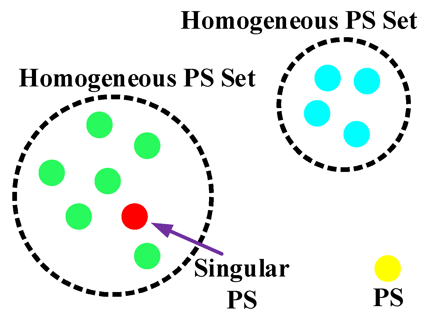
PSs belonging to each structure (e.g., a building) can be easily selected by using a database of the building location and shapes. In order to ensure that almost all PS on each building would not be omitted, we can add a small (depending on the PS position precision) buffer area outside the original building areas. Then, for each structure (which can contain from zero to a very high number of PSs), we apply a hierarchical clustering method (see Figure 1) in order to identify homogeneous PS sets (other clustering approaches have been presented in [28,29,30]). Two PSs can be considered as belonging to the same homogeneous set if the Euclidean distance between their spatial positions and the deviation between their displacement temporal evolutions are smaller than the given thresholds, respectively. The deviation between two PS displacement histories can be calculated according to the following equation:

$$B=\left({\sum }_{i=1}^M{(X_i-Y_i)}^2\right)/M$$

(1)

where $M$ is the number of temporal samples and $X_i$ and $Y_i$ are the displacement values of the two PSs, respectively, at the ith acquisition time. Based on the theory of random signals, if the two PSs are similar, we can assume that $X_i-Y_i$ has a Gaussian distribution, namely $X_i-Y_i~N\left(0,{\sigma }^2\right)$, and $MB/{\sigma }^2$ has a chi-squared distribution, namely $MB/{\sigma }^2~{\mathsf{\chi }}^2\left(M\right)$. Generally, ${\sigma }^2$ is related to the noise levels of the two PSs, and it could be estimated in advance. We could eventually calculate the deviation threshold based on chi-squared test theory.

After homogeneous PS set identification, we can isolate and remove the so-called false or singular PSs. The criterion to detect a singular PS is that the PS is near to a large homogenous PS set, but its displacement temporal evolution is very dissimilar from that of the homogenous PS set. Practically, we can identify the singular PS by determining whether the Euclidean distance between the isolated PS (potential singular PS) and the centroid of each large homogeneous PS set (it should contain a certain number of PSs) is within a given threshold.

Finally, after removing the singular PSs, for each homogeneous PS set, a single convergence point can be defined, characterized by geographical coordinates, and its displacement evolution obtained by averaging those of all PSs in the homogeneous PS set. The remaining isolated PSs (the yellow PSs in Figure 1) can also be defined as convergence points.

In the successive steps of the proposed approach, we use only the obtained convergence points in order to perform the building stability analysis. By considering only the convergence points, we can reduce the number of displacement measurements to be analyzed, and at the same time, increase their reliability.

2.2. Classification of Buildings and Detection of Spatially Anomalous Deformations

Considering the number and the spatial distribution of the obtained convergence points, each analyzed structure can be classified into one of four different categories (see

Table 1. Different building categories depending on the deformation information provided by satellite synthetic aperture radar interferometry (InSAR) measurements.

Building Type	Instruction	Maximum Measured Settlement (dmax)	Maximum Measured Differential Settlement (${\Delta }_{d,max}$)	Maximum Measured Angular Distortion (βmax)
0	No convergence point	X	X	X
I	Only one convergence point	✓	X	X
II	At least two convergence points	✓	✓	X
III	At least a pair of convergence points at similar heights	✓	✓	✓

):

• Type 0 structures have no convergence points. Therefore, no stability analysis can be performed.
• Type I structures have just a single convergence point. Consequently, in such a case, the displacement value of the identified convergence point will be used to evaluate the structure settlement.
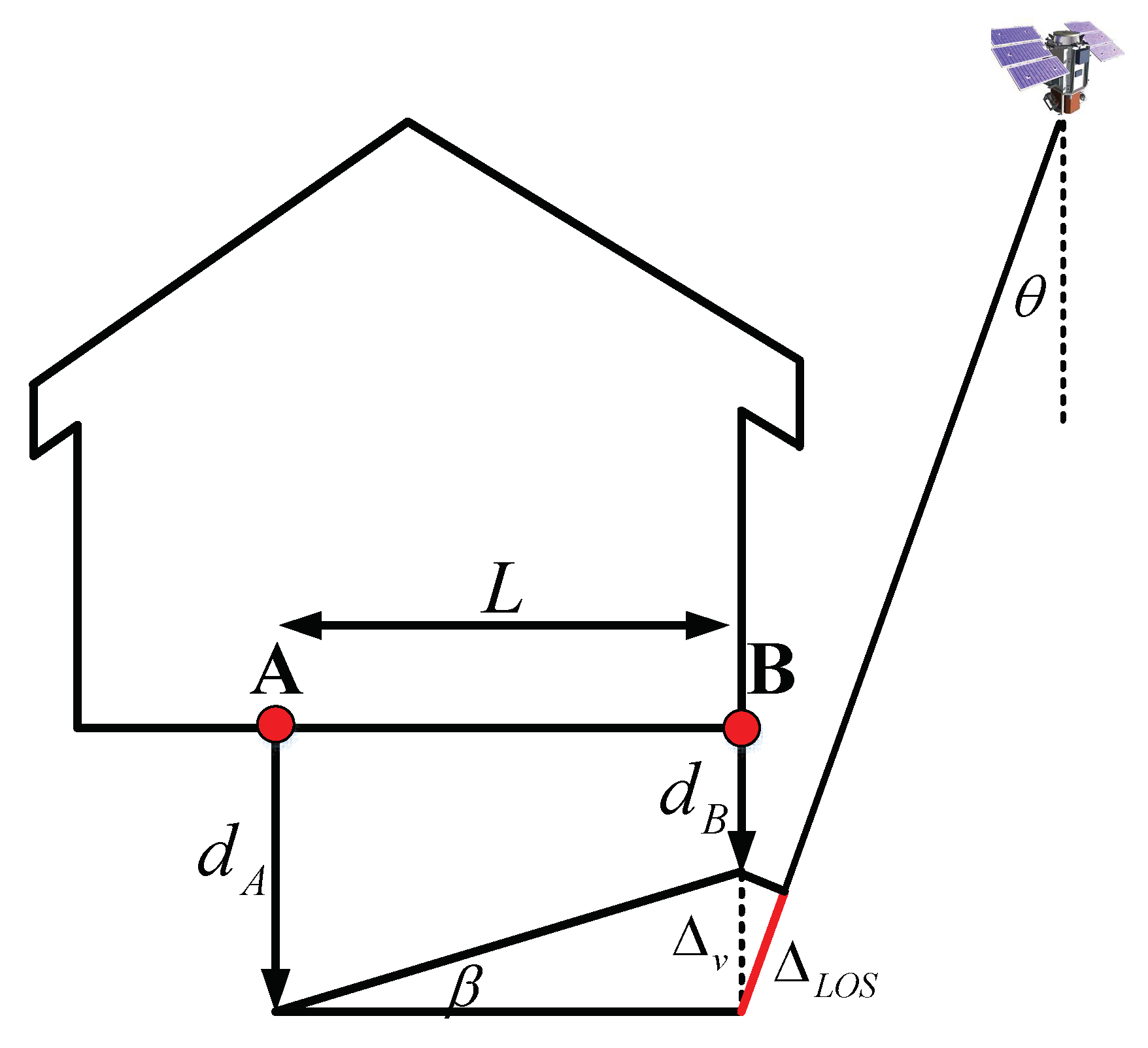
• Type II structures have at least two convergence points. For such a building, we can use two different criterions to identify potentially dangerous situations: the maximum measured settlement value and the maximum measured differential settlement value (see Figure 2 and the related explanation).
• Type III structures have at least a pair of convergence points with similar heights. In these cases, we can consider for the stability analysis also the value of angular distortion β (see Figure 2 and the related explanation). It is worth noting that the roof and the foundation can have different deformation trends even when no building tilting occurs. Therefore, the angular distortion can be calculated only by considering two points with similar heights.

The proposed method evaluates the building stability by comparing the previously described parameters with proper thresholds, and obviously, the higher the number of available parameters there are, the more reliable the analysis result will be.

It is worth showing (Figure 2) how differential settlement and angular distortion can be easily derived from InSAR measurements [31]. The differential settlement ${\Delta }_d$ is the difference of the vertical displacement component between two convergence points. We calculated the value by using the following equation (for convenience of description, the differential deformation is defined to be negative):

$${\Delta }_d=-\left|d_{A,LOS}-d_{B,LOS}\right|cos{\theta }_{inc}=-\left|{\Delta }_{LOS}\right|/cos{\theta }_{inc}$$

(2)

where d_A,LOS and d_B,LOS are the displacements measured on the convergence points A and B, respectively, along the satellite LOS (Line of Sight) direction during the monitoring period; Δ_LOS is the absolute value of difference between these two measurements; and θ_inc is the satellite incidence angle. It is worth highlighting that the Δ_LOS value is divided by the cosine of the satellite incidence angle in order to obtain the vertical differential settlement ${\Delta }_d$.

The angular distortion β we consider is related to the measured vertical differential settlement, and it is computed as the ratio between ${\Delta }_d$ and the distance L between the two convergence points:

$$\beta =-{\Delta }_d/L$$

(3)

It is worth pointing out that the angular distortion value must be calculated only between points with similar height values. In fact, it is normal that the deformation on the roof and foundation can differ from each other even for stable structures.

2.3. Detection of Spatially Anomalous Deformations: Real Data Analysis

In this section, we report the results obtained by applying the method described in Section 2.1 and Section 2.2 to a real test case. In particular, we used the proposed method for the identification of spatially anomalous deformations to assess the stability of a building in Foshan, China. A set of 57 COSMO-SkyMed stripmap SAR images acquired from 17 February 2013 to 14 January 2018 were processed by using the PSP InSAR algorithm [8]. 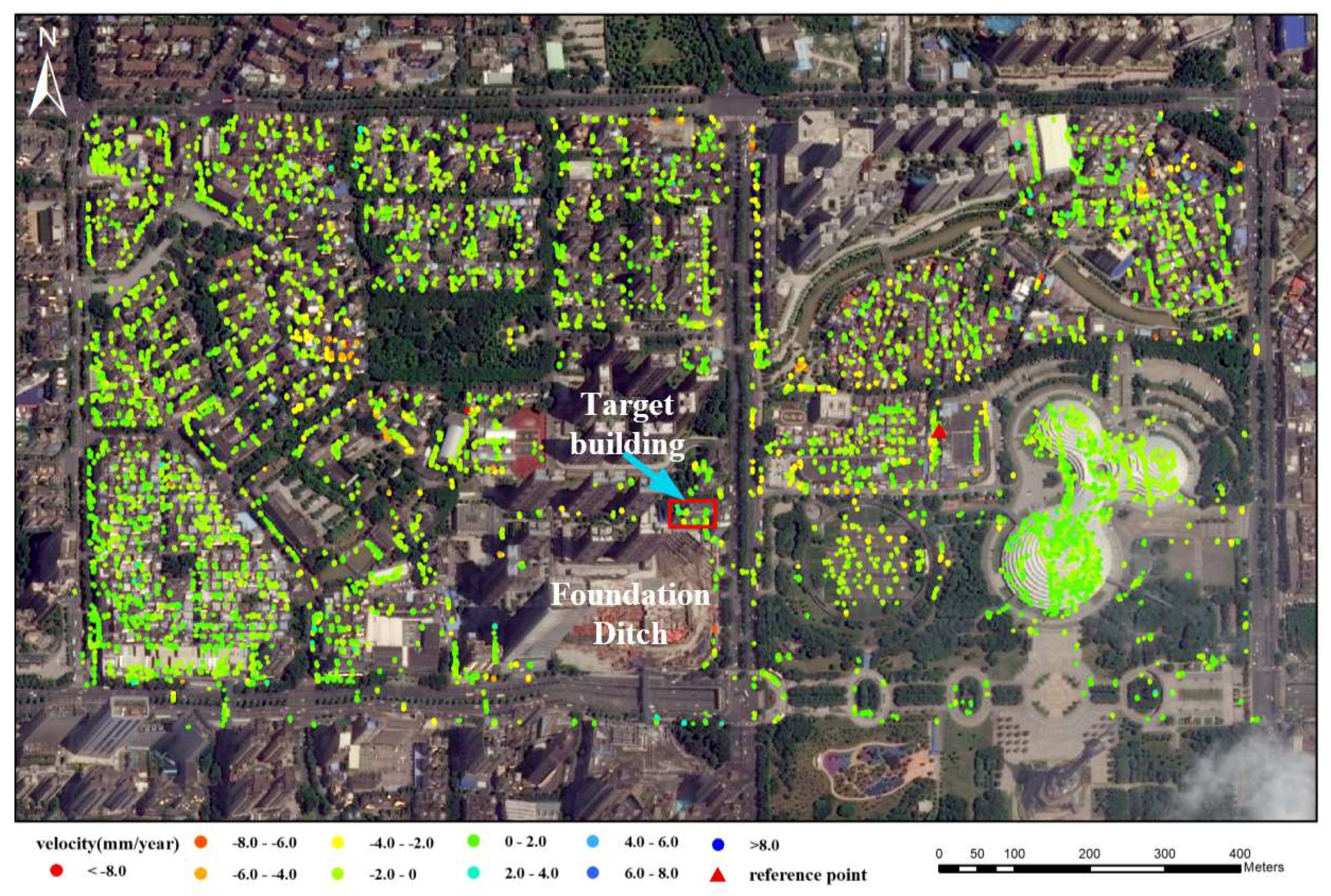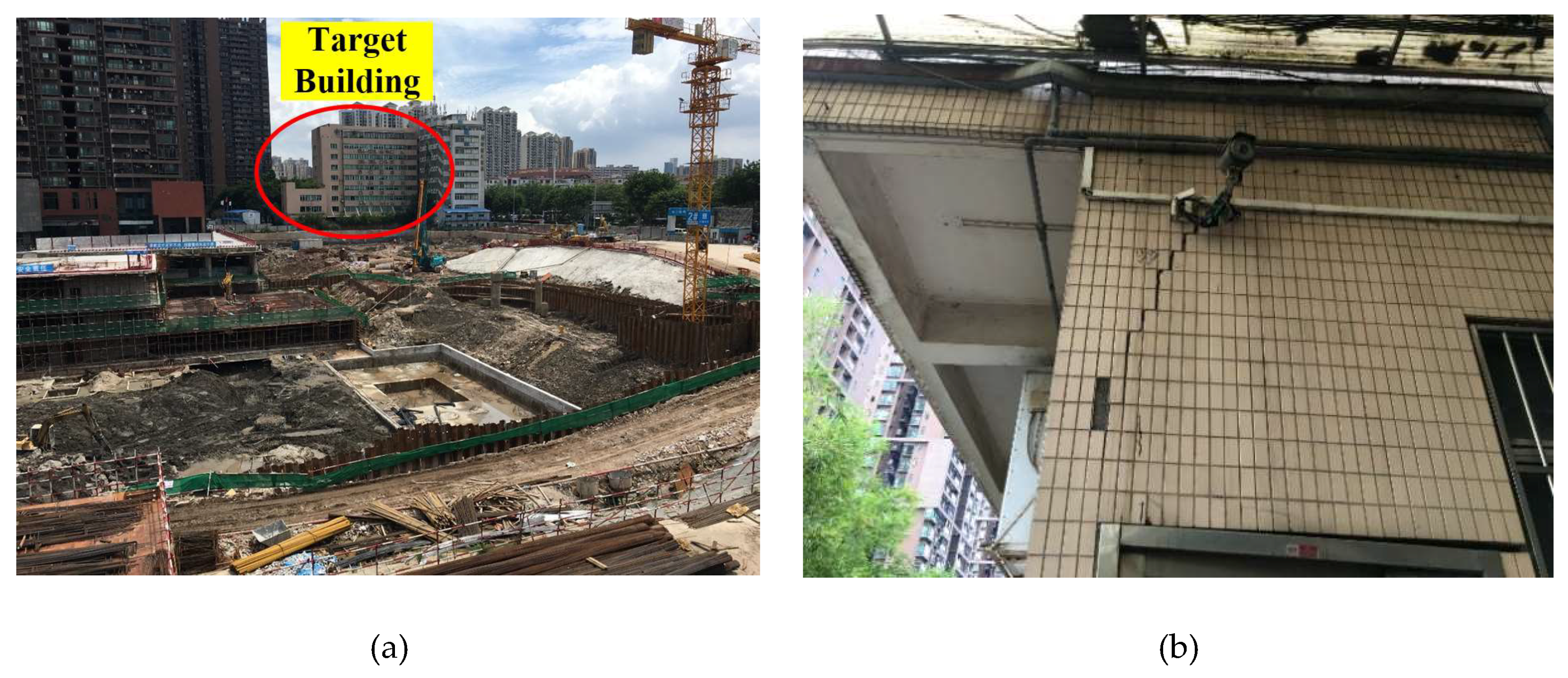Figure 3 shows the mean velocity map of the PSs found in the considered area and the target building.

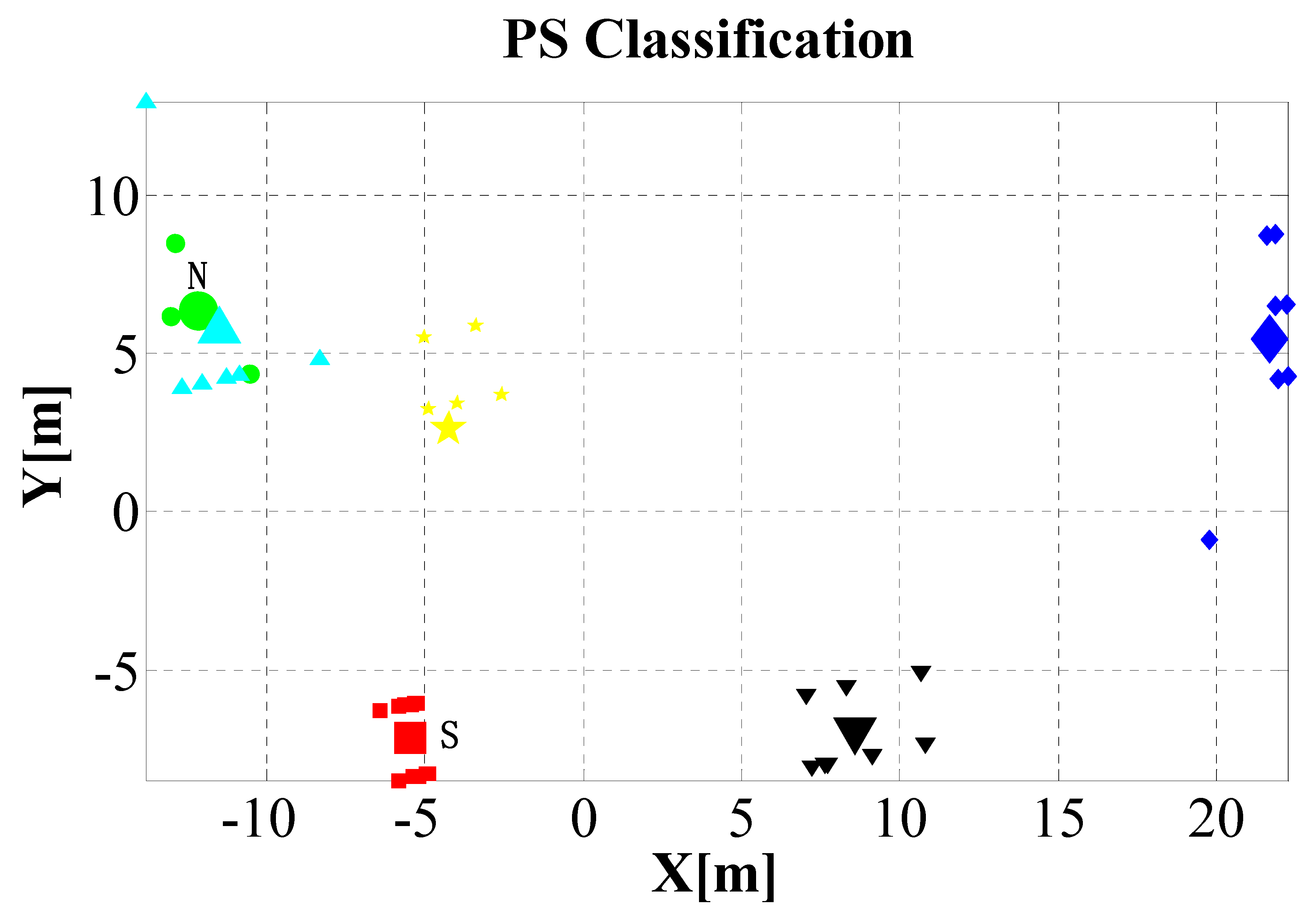
Figure 4 shows the PSs selected over the target building (small points) and the convergence points obtained from them (big points). Since pairs of convergence points with similar heights were detected on the building (meaning it is a type III structure), we could compute from the satellite measurements the maximum settlement d_max, the maximum differential settlement ${\Delta }_{d,max}$, and the maximum angular distortion β_max of the building. The two homogenous PS sets with the largest differential settlement were identified and marked by N (north) and S (south), respectively.

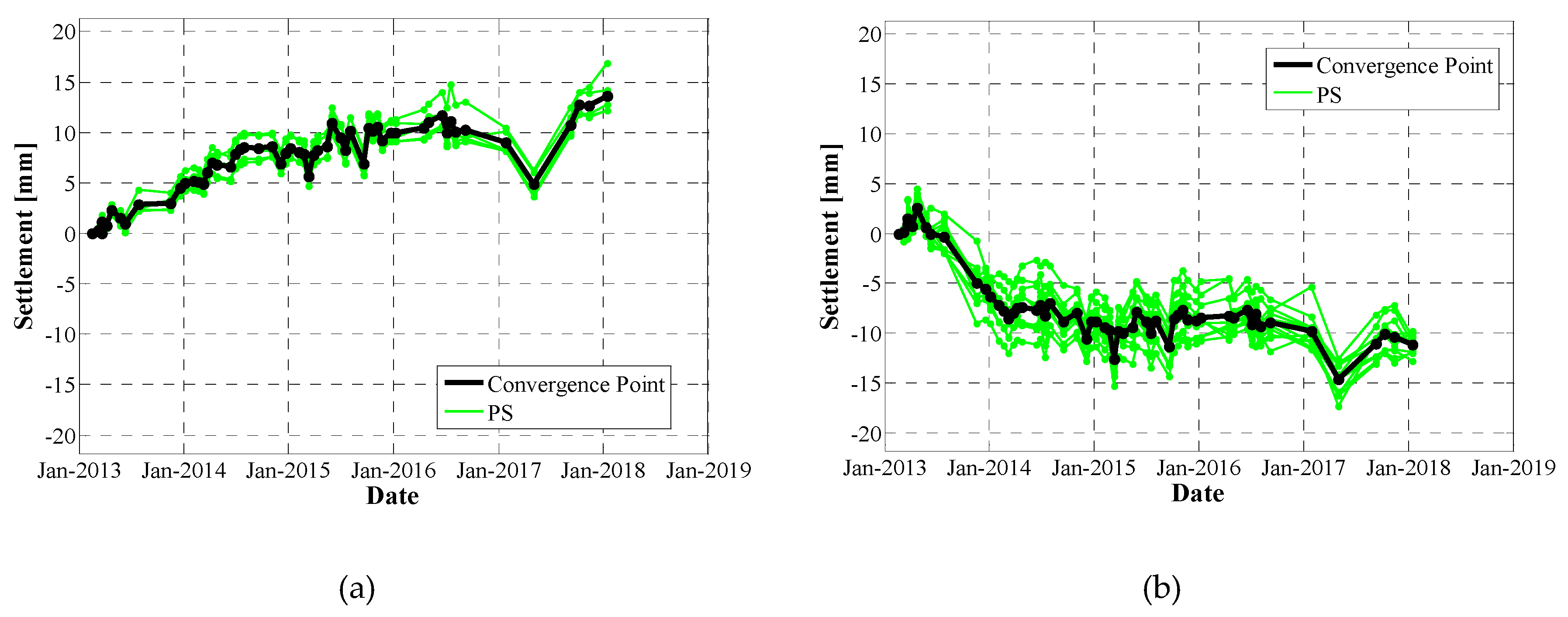
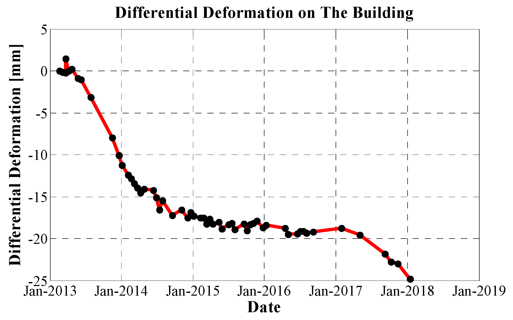
Figure 5 shows the settlement evolutions of the PSs belonging to these two sets and of their corresponding convergence points. It can be clearly observed that the points in the N set were uplifted (positive value), whereas the points in the S set subsided (negative value) in the monitoring periods (February 2013 to January 2018), with a maximum measured differential settlement ${\Delta }_{d,max}$ of −24.8 mm (Figure 6). The corresponding angular distortion β_max is 2.4‰ (which is a large value for general buildings). Even though the maximum measured settlement value was not very high, since both the maximum measured differential settlement and the maximum measured angular distortion were very large, the analyzed building was considered as potentially being in danger. This analysis was confirmed by a field survey, in which we obtained some photographic evidence (see Figure 7) showing cracks on the building.

3. Deformation Evolution Decomposition and Detection of Anomalous Temporal Trends

3.1. Temporal Deformation Model

Generally, displacements of structures do not evolve linearly with time. For example, subsidence is related to underground water or gas extraction/injection activities, which can happen at specific times and with different intensities. Also, during periods of building and infrastructure construction, larger deformations are often observed on targets near the construction areas. Moreover, seasonal deformation phenomena are present, with thermal expansion and contraction particularly evident on skyscrapers, bridges, and so forth.

In order to facilitate the analysis of PS nonlinear movements, we consider the following multiple linear regression model with m breaks (m + 1 partitions):

$$\{\begin{array}{c}{d}_i=v_1{t}_i+b_1+Asin(2\pi t_i+\phi )+{\epsilon }_i,i=N_0,N_0+1,\dots ,N_1\\ d_i=v_2{t}_i+b_2+Asin(2\pi t_i+\phi )+{\epsilon }_i,i=N_1+1,N_1+2,\dots ,N_2\\ \cdots \\ \cdots \\ \cdots \\ d_i=v_{m+1}{t}_i+b_{m+1}+Asin(2\pi t_i+\phi )+{\epsilon }_i,i=N_m+1,N_m+2,\dots ,N_{m+1}\end{array}$$

(4)

In this model, d_i are the observed deformation values at the ith acquisition time t_i. (i = N₀, N₀ + 1, N₀ + 2…, N_m+1); ν_j and b_j, (j = 1, 2, …, m + 1), which represent the velocity and constant deformation of the jth partition, respectively, are the coefficients of the piecewise linear deformation component; A and φ are the corresponding coefficients of the periodical deformation component, which are assumed to be the same during the whole monitoring period; ε_i is the random noise at the ith acquisition time; and (N₁, N₂, …, N_m) are the indices of m break points, which are explicitly treated as unknowns.

The periodical component describes a regular movement of expansion and contraction, and the amplitudes are different for different targets. On the contrary, the piecewise linear component represents the deformation trend at each temporal partition, and it can be important to evaluate the stability of the target. Note that for most PS points, thermal dilatations are the main source of the periodical component typically observed in the PS displacement evolution curves. Since the purpose of our deformation evolution decomposition procedure is to analyze trend variations, the component of the deformation signal correlated to the temperature variations represents a disturbance in our analysis and should be isolated and removed. Thermal dilatation phenomena are directly correlated to temperatures, which change in both the temporal and spatial dimensions. In general, it is difficult to acquire accurate temperature data for each point and time from external sources. We then use an approximated model (sinusoidal) to estimate this periodical component from the InSAR measurements. Obviously, if the deformation on the analyzed target followed other periodical rules, we would have to replace the sinusoidal model with a more appropriate one.

3.2. Deformation Evolution Decomposition and Anomalous Trend Detection

Given model (4), the goal is to estimate the unknown regression coefficients (ν_j, b_j, A, and φ), together with the indices of break points (N₁, N₂, …, N_m), when the deformation measurements d_i at the ith acquisition times are available. The decomposition process is based on an iterative least-squares procedure. For each possible choice of partition (N₁, N₂, …, N_m), the estimated parameters $\widehat{v}$_j, $\widehat{b}$_j, $\widehat{A}$, and $\widehat{\phi }$ can be obtained by minimizing the following objective function, i.e., the sum of squared residuals:

$$S(N_1,N_2,\dots ,N_m)={\sum }_{j=1}^{j=m+1}{\sum }_{k=N_{j-1}+1}^{k=N_j}{(d_k-v_j{t}_k-b_j-Asin\left(2\pi t_k+\phi \right))}^2$$

(5)

Therefore, the estimated breaks are:

$$({\widehat{N}}_1,{\widehat{N}}_2,\dots ,{\widehat{N}}_m)=\mathrm{argmin}{S}_N\left(N_1,N_2,\dots ,N_m\right)$$

(6)

As the breaks are discrete parameters, we can use a grid search method [32]. In the searching process, the break number m is unknown at the beginning. In order to estimate it, we gradually increase the value of m from zero, and stop the iteration when the sum of the squared residuals, S, is lower than a certain threshold, or when the number of breaks, m, is larger than certain threshold. The minimum length of each temporal interval and the maximum number of breaks can be adapted based on the characteristics of the specific PS: the higher the noise level of the PS displacement measurement is, the larger the minimal length of each temporal partition and the smaller the maximum number of partitions (m) should be. Generally, the noise level of a single PS is much higher than the one of a convergence point. Therefore, by using the convergence points instead of single PSs, it is possible to consider them as reliable shorter temporal partitions, which can help detecting more abrupt changes.

The optimization problem defined above can be solved in a computationally efficient way by exploiting the dynamic programming technique [32]. In the following, we list the main steps of the recursive procedure implemented to estimate the parameters of the multiple linear regression model:

(1)

Set m = 0;

(2)

Estimate the multiple linear regression model:

a)

Set V = [v₁, v₂, …, v_m+1] and B = [b₁, b₂, …, b_m+1] vectors to zero;

b)

Compute the residual deformation after removing the piecewise linear model (based on the current m, V, and B values) from the original measured deformation;

c)

Estimate the periodic component coefficients A and φ on the obtained residual deformation component;

d)

Compute the residual deformation after removing the periodic deformation component (based on the current A and φ values) from the original measured deformation;

e)

Apply the dynamic programming method to the residual deformation without periodical component in order to estimate the vectors V, B, and N_break = [N₁, N₂, …, N_m];

f)

Repeat steps (b–e) until N_break = [N₁, N₂, …, N_m] does not change anymore;

(3)

Calculate the objective function value (see Equation 5), and if it is greater than a given threshold, add one to m and go back to Step (2).

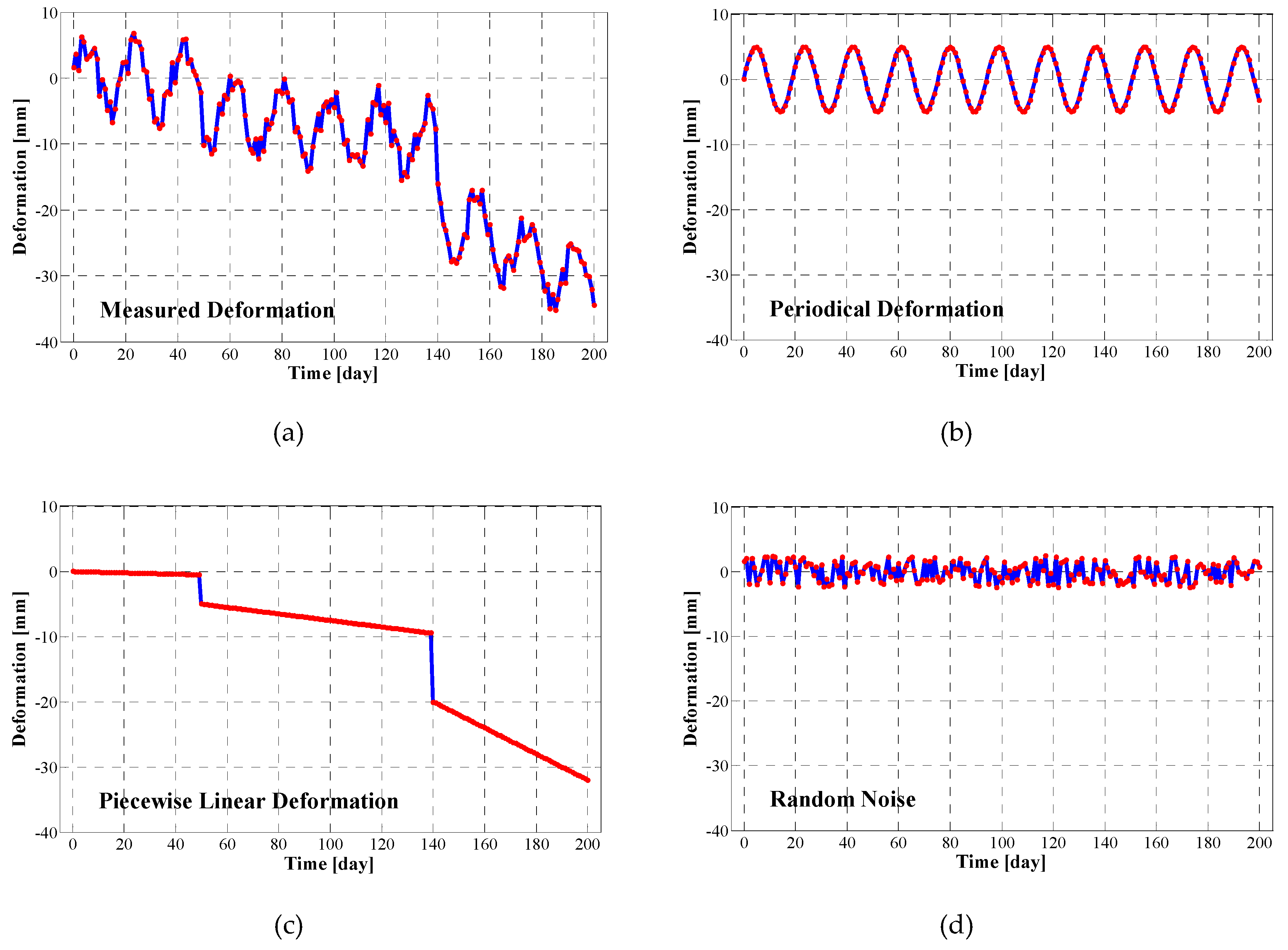
An example of decomposition based on simulated data is shown in Figure 8. The recursive procedure retrieves information on the periodical component and trend variations that have occurred on the analyzed structures.

For each PS or convergence point, the piecewise linear component decomposition provides the mean velocity of the deformation for each temporal interval and it can be used to detect a potentially critical situation in the temporal dimension. To analyze structure stability in the temporal dimension, we can use the mean velocities computed either considering the entire temporal series of measurements or only the most recent measurements. In particular, if one of these two parameters become larger than a given threshold, the corresponding structure can be considered as potentially being in danger. Again, as already observed in Section 3, the usage of more parameters allows to increase the capability of detecting anomalous trends.

3.3. Anomalous Trend Detection: Real Data Analysis

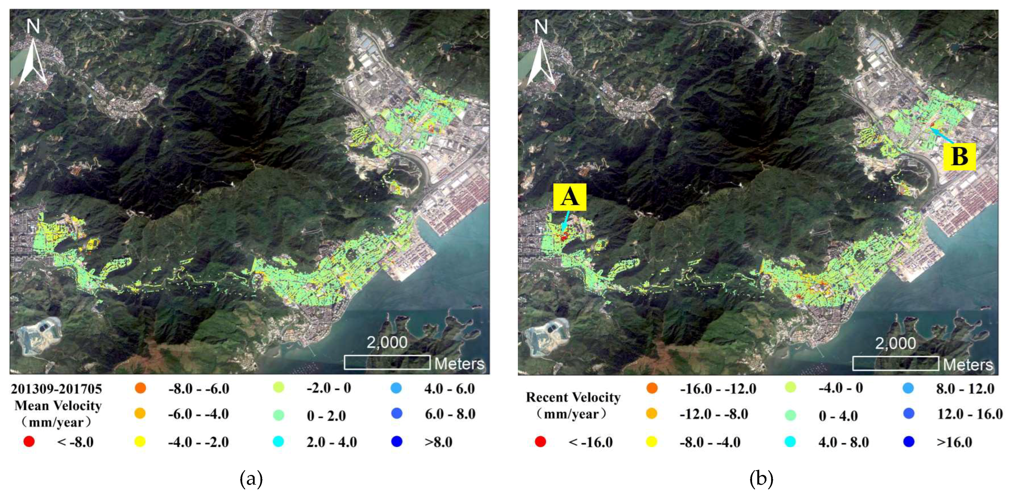
This section presents the results obtained applying the temporal analysis procedure described in Section 3.1 and Section 3.2 to the InSAR-measured deformations along a subway line in Shenzhen, China. The subway construction started from Dec 2016. The deformation information was obtained by PSP InSAR processing [8] of a set of 57 stripmap COSMO-SkyMed SAR data acquired in the period 14 September 2013–28 May 2017.

Figure 9a shows the PS mean velocity measurements relative to the whole observation period along the subway line. By observing only the mean velocity map relative to the whole analyzed period, no evidence of significant deformation in the study area is visible. In reality, thanks to the temporal analysis described above, it is possible to identify areas or points affected by significant trend variation. 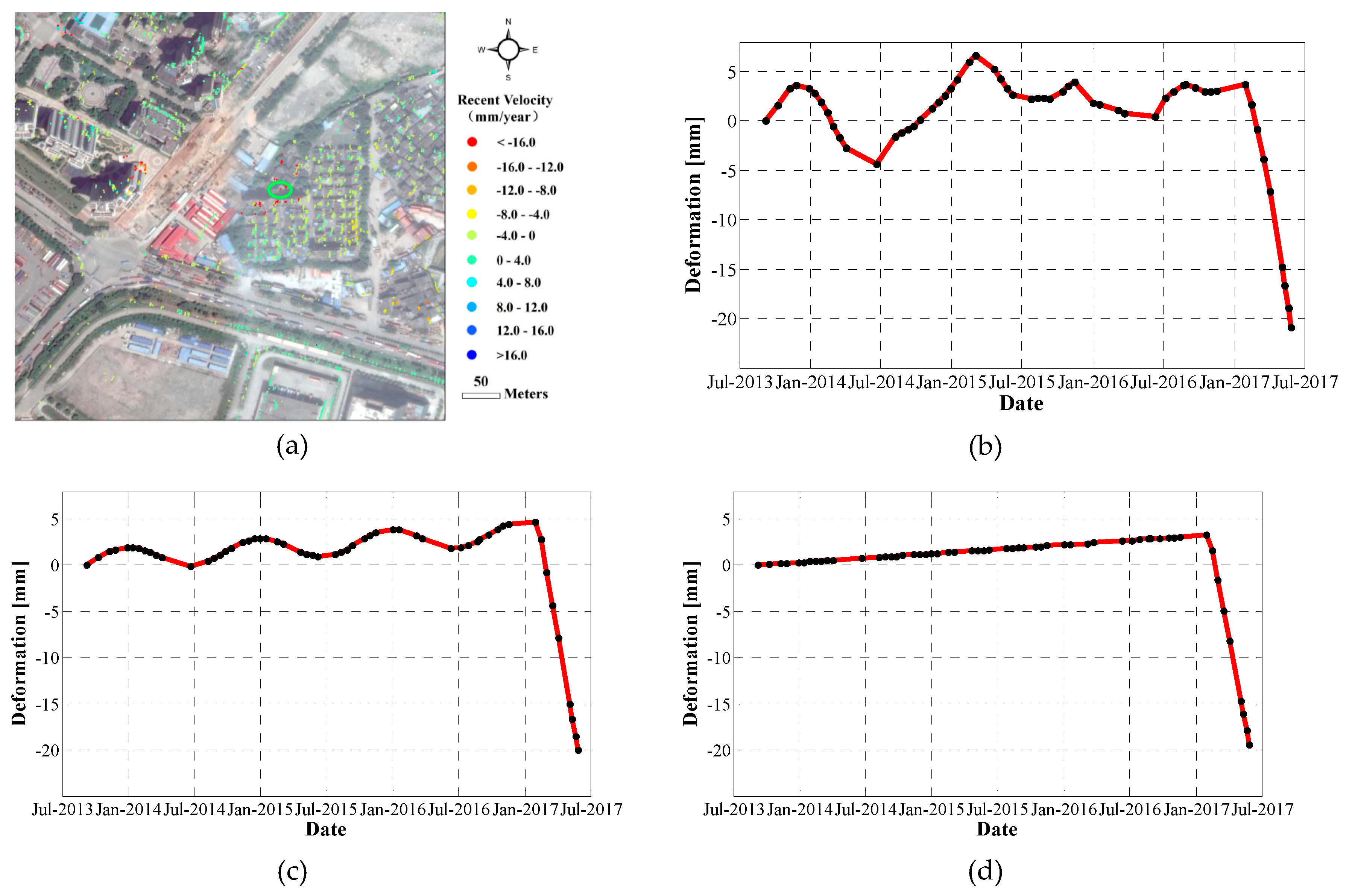Figure 9b shows the PS recent velocity (the velocity in the last partition), where it is possible to observe several areas affected by significant deformation, especially for the two areas marked as A and B.

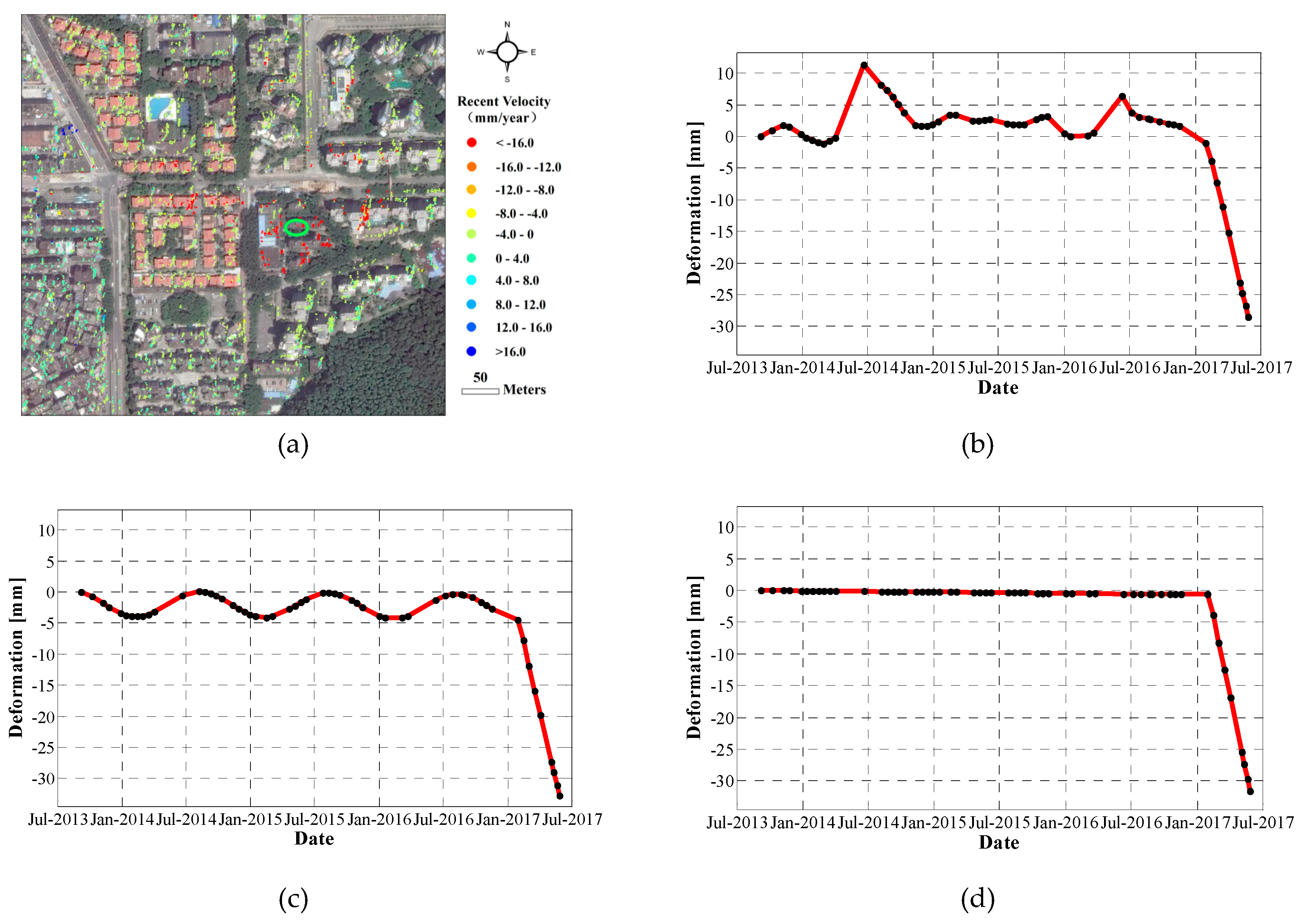
By analyzing the deformation temporal evolution thoroughly, we can find more information. For the area A, the decomposition results of one selected PS is shown in Figure 10. A slight periodic deformation component is visible on the multiple linear regression model (sum of periodic and piecewise linear components of the PS displacement) shown in Figure 10c. Furthermore, when observing its piecewise linear component as shown in Figure 10d, we can conclude that there are two partitions for the PS deformation temporal evolution, and the exact break time is between Dec 2016 and Jan 2017. Before the break time, almost no displacement is observed, whereas after that date, the velocity increases to 48 mm/year. For the area B, a similar phenomenon can be observed, which is shown in Figure 11.

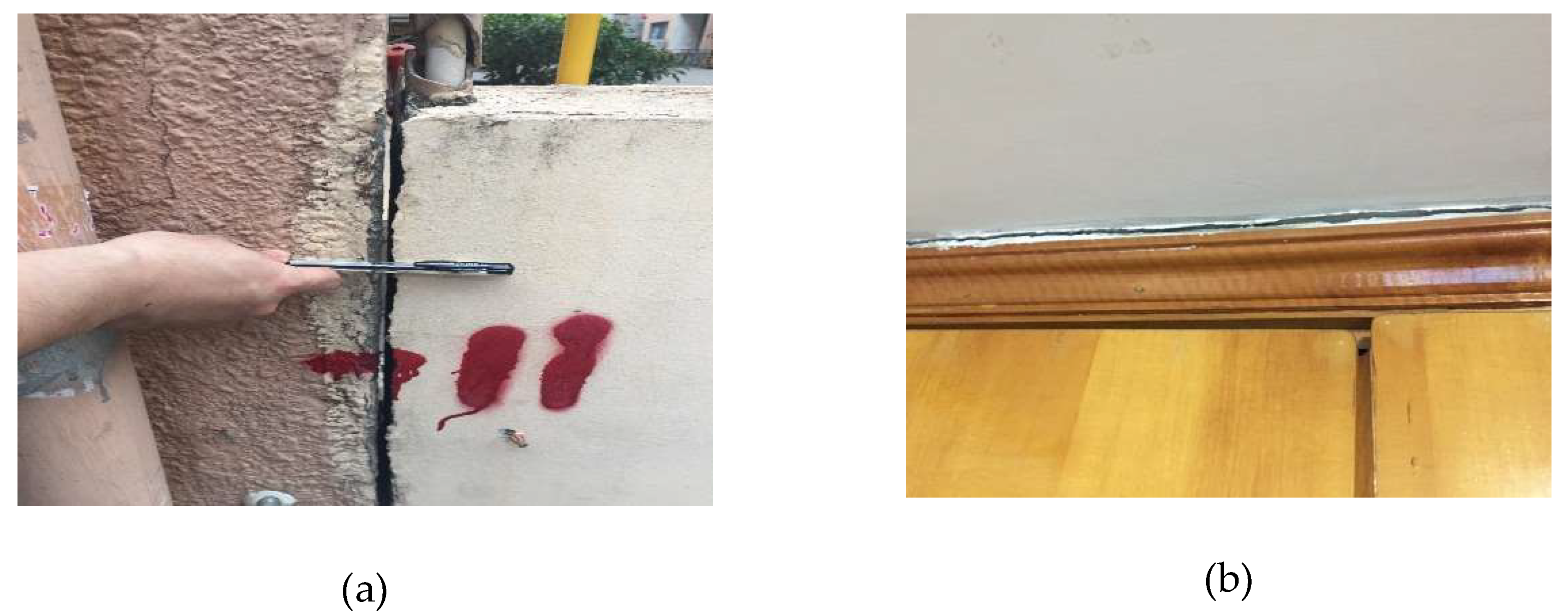
As mentioned above, the subway construction in the study area started in Dec 2016, which corresponds to the break time found by our automatic temporal analysis of the InSAR measurements. Therefore, the velocity variation can be attributed to the subway construction process. A field survey in area A was performed, and big cracks were found both outside and inside the building (as shown in Figure 12), which confirmed the severe consequences caused by the anomalous deformation.

4. Automatic Analysis of Large Areas for Building Stability Assessment

4.1. Building Stability Assessment System

Based on the spatial and temporal analysis method described in Section 2 and Section 3, we have built a processing system to automatically evaluate building stability from InSAR measurements. Figure 13 shows the flowchart of the processing chain. For each building, the PSs found by the InSAR processing are clustered into different homogenous sets, and then the corresponding convergence point is computed for each homogenous set. The next step is the building classification, relying on the number and geometric distribution of the convergence points. By using these convergence points, it is possible to assess the building stability by applying the method of the spatially anomalous deformation detection. Then, the temporal evolutions of the most relevant convergence points are analyzed using the temporal decomposition method. If one of the spatial or temporal dimension analyses detect an anomaly, the building will be identified as potentially being in danger. Clearly, the final alarm level of a structure will be obtained from the joint analysis of all the different risk parameters (both in the spatial and temporal dimensions), which largely improve the stability evaluation’s capability.

4.2. Building Stability Assessment on Real Data in Large Areas

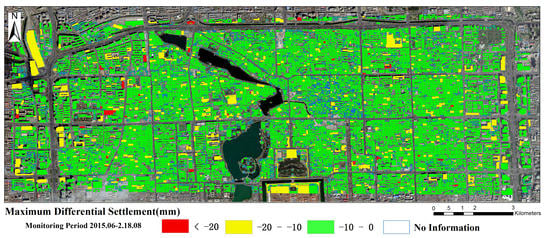
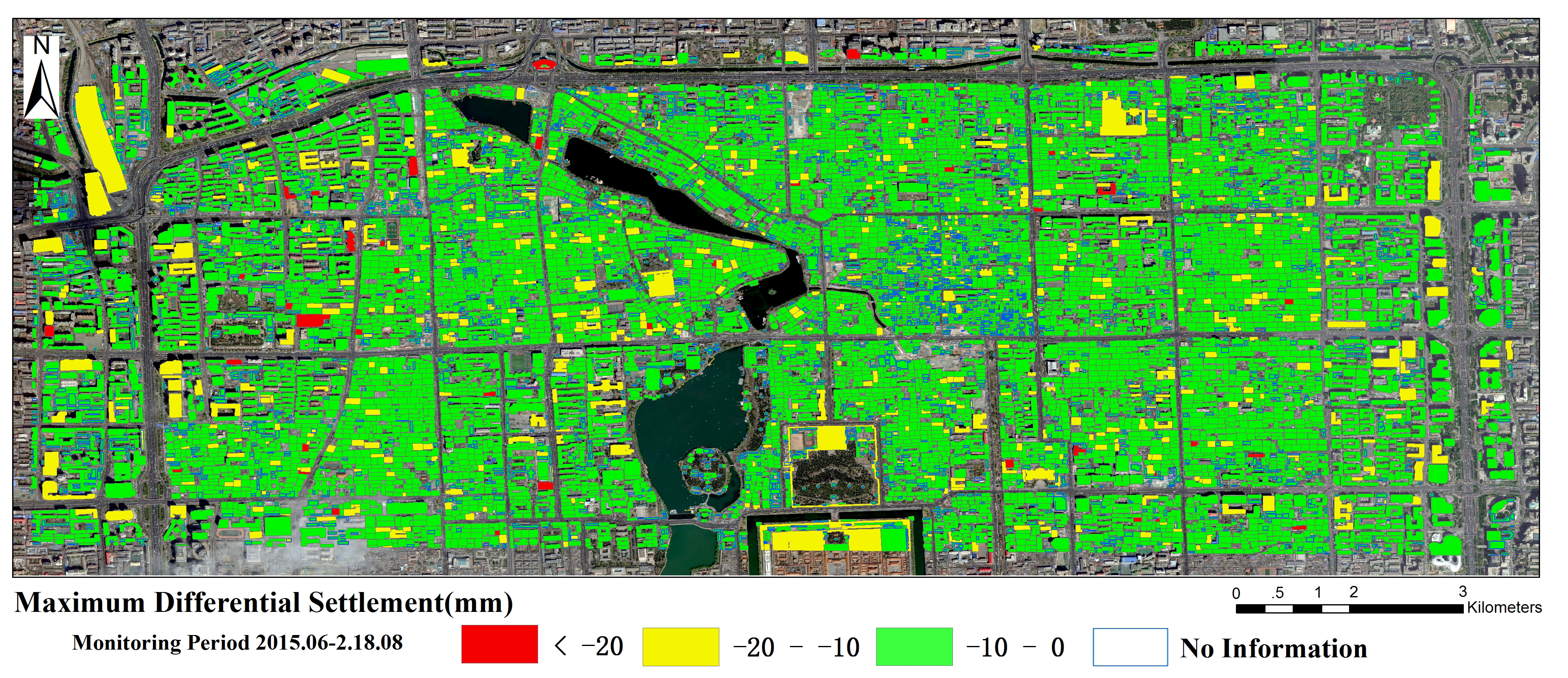
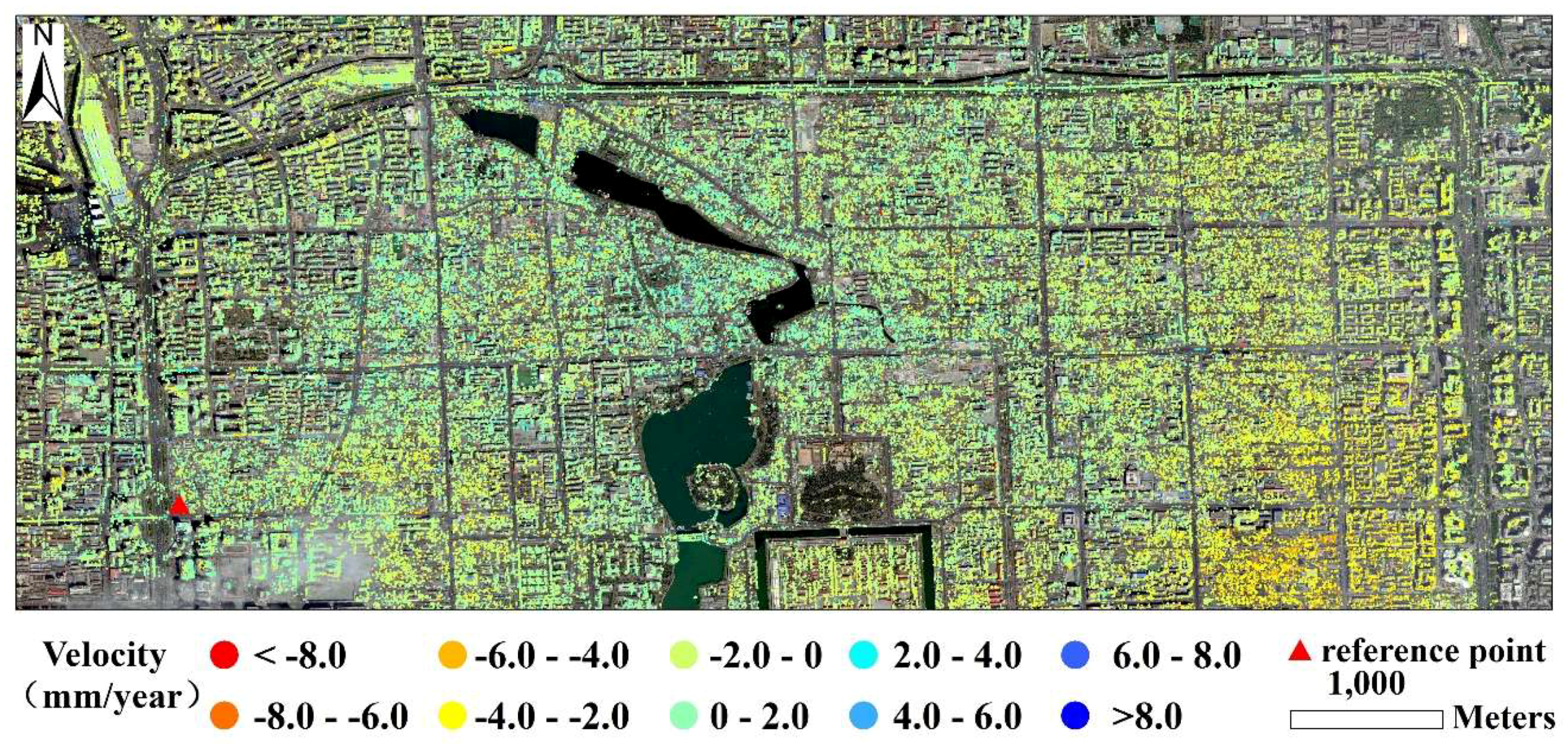
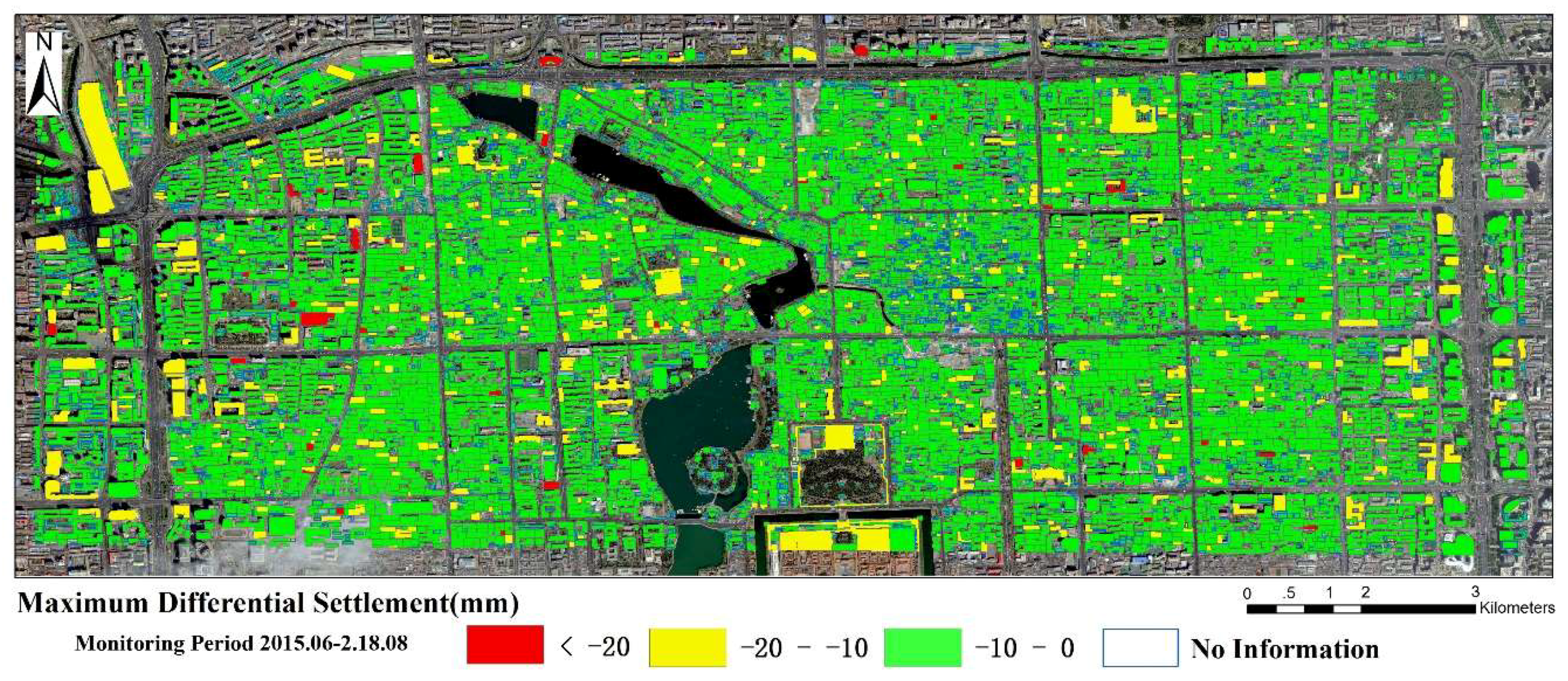
In order to test our building stability assessment method on a large area, we considered the city of Beijing, China. A stack of 32 COSMO-SkyMed (CSK) SAR images (stripmap mode, 3 m × 3 m resolution), acquired from June 2015 to August 2018, were processed by the PSP InSAR technique [8]. A total of 524,873 PSs were found. Figure 14 shows the PS mean velocity (relative to the entire monitoring period) map.

As described in Section 2.2, the proposed method allows to assess the stability of structures that belong to type I, II, or III, as described in Table 1. Thanks to the high density of COSMO-SkyMed PSP InSAR measurements, most of the 12,272 buildings in the considered area of Beijing contained at least one PS and could be analyzed. In fact, just the 9.7% of buildings were type 0 structures. The complete classification of buildings for this case study is shown in

Table 2. Building number for each type.

Building Type	Building Number	Percentage
Type 0	1192	9.7%
Type I	4771	38.9%
Type II	357	2.9%
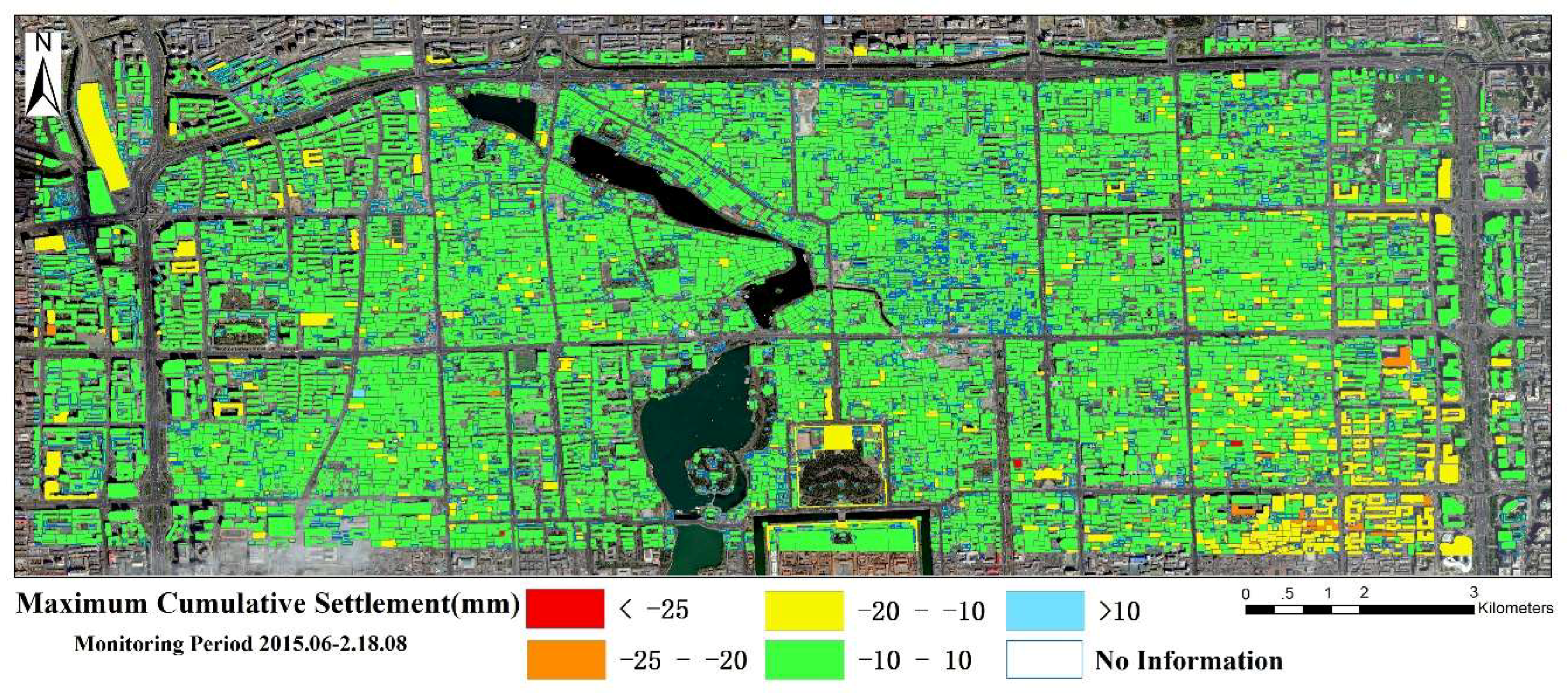
Type III	5952	48.5%

. On all the type I, II, or III structures, we were able to compute the maximum measured settlement value, obtaining the map shown in Figure 15. In the maximum measured settlement map (Figure 15), positive values correspond to uplift phenomena, whereas negative values correspond to subsidence phenomena. On type II and III buildings, we could also compute the maximum measured differential settlement (because the value is always negative, the smaller the differential settlement is, the higher the risk level corresponding to the building is). Figure 16 shows the corresponding map.

In the following, we present some examples of the results obtained for buildings that differ in terms of height and construction date. On these buildings, we compared the results obtained by using the proposed automatic method for building stability assessment (based on PSP InSAR measurements) with in situ evidence, in order to validate the effectiveness and reliability of the proposed technique.

4.2.1. Building 1

The first example (see Figure 17) is relative to a 6-floor residential building built in the 1990s. The building is about 18 m tall and has an area of about 750 m². Based on the InSAR results, the building was classified as a type III structure (see Table 1) and we were able to compute its maximum settlement, maximum differential settlement, and angular distortion factor. We computed a maximum mean annual velocity of about −11.9 mm/year in the monitoring period of June 2015–August 2018, which corresponds to a cumulative settlement d_max of about −35.5 mm. The maximum measured differential settlement ${\Delta }_{d,max}$ was about −26.9 mm. The obtained maximum angular distortion β_max was about 2.0‰ (quite close to the threshold that is normally used in China to consider a building as being affected by some instability issue). Moreover, by analyzing the settlement trend, it could be observed that the differential settlement value was gradually increasing in the temporal interval of our satellite measurements.

The obtained results showed the presence of significant settlement phenomena on the building and suggest that its stability should be monitored more deeply. The conclusion obtained from our building stability assessment from satellite InSAR measurements was confirmed by the in-situ investigations performed in August 2018. The pictures showed vertical cracks on the northwestern facade of the building.

4.2.2. Building 2

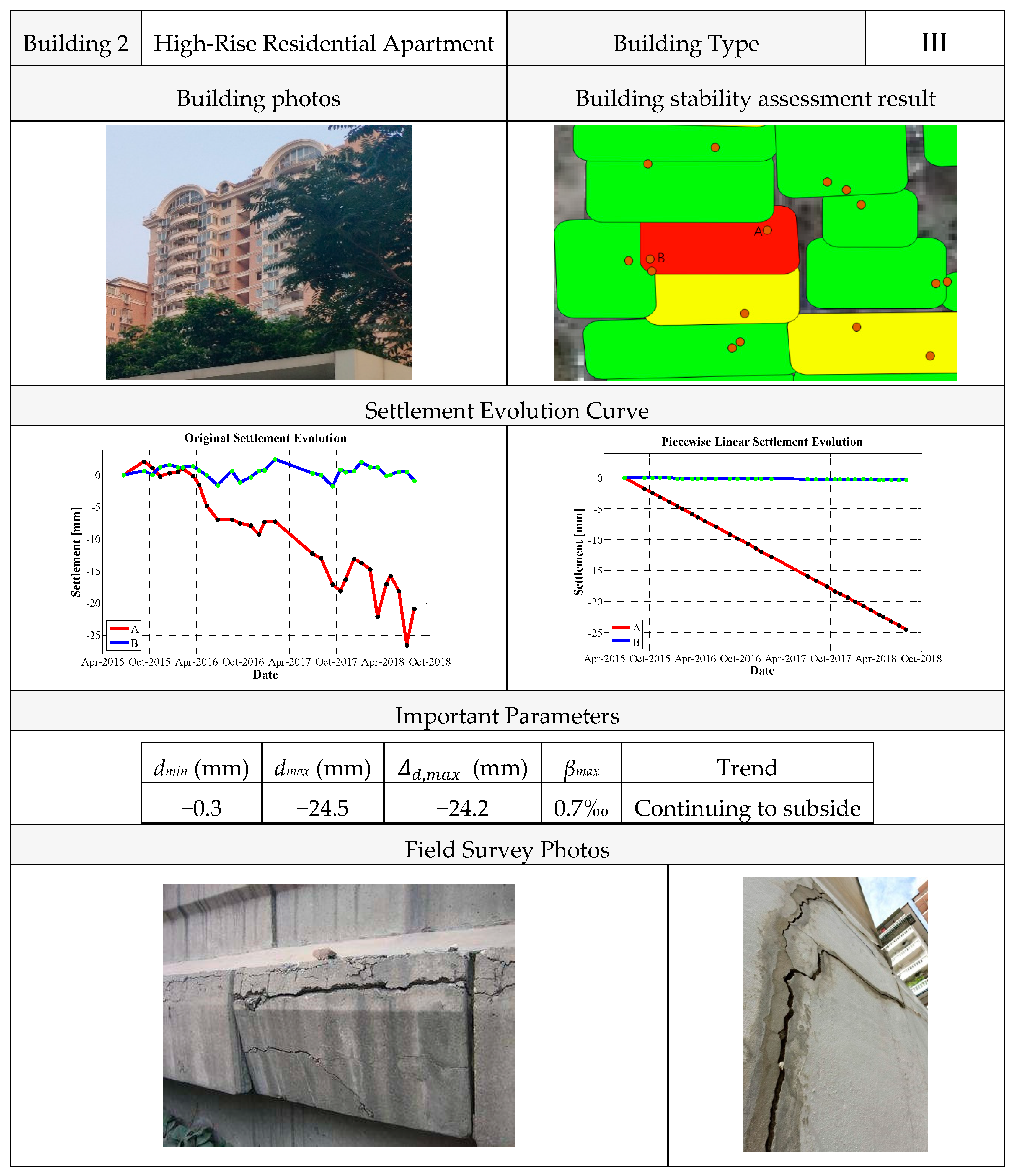
The second building analysis (see Figure 18) example refers to a residential building erected in 2010, having a height of 63 m and covering an area of about 1200 m². Based on the InSAR results, the building was classified as a type III structure (see Table 1). We could compute a cumulative settlement d_max of about −24.5 mm, a maximum measured differential settlement value ${\Delta }_{d,max}$ of −24.2 mm, and a maximum measured angular distortion value β_max of about 0.7‰. Moreover, by the analysis of the deformation trend, it could be noted that the differential settlement was continuing to increase in the analyzed temporal interval.

The performed analysis pointed out the need to evaluate the stability conditions of this building more deeply. This conclusion was also confirmed by the in situ investigations that uncovered evidence of settlement phenomena (i.e., vertical cracks on the external walls of the southern part of the building).

4.2.3. Building 3

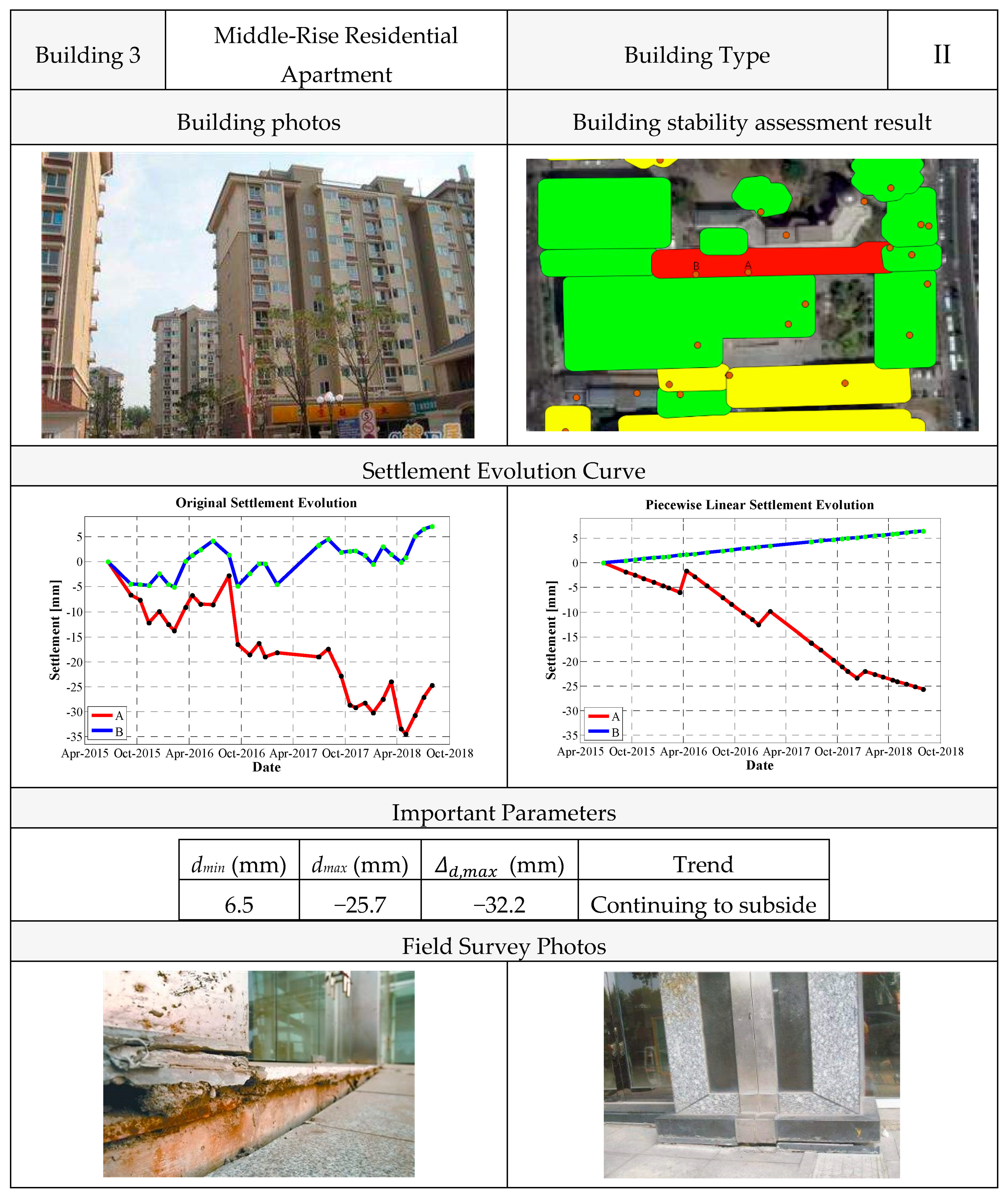
The third example reported in this paper (see Figure 19) refers to a residential building constructed in the 2000s, having a height of about 30 m and an area of about 1500 m². Based on the InSAR results, this building was classified as a type II structure (see Table 1). From the satellite measurements, we were able to estimate the maximum settlement and the maximum differential settlement (whereas the angular distortion factor could not be computed). We calculated a cumulative settlement d_max of −25.7 mm and the maximum differential settlement ${\Delta }_{d,max}$ of about −32 mm. Moreover, by the analysis of the deformation trend, it could be noted that settlement rate persisted over the whole observation period.

Again, the result of the performed analysis, confirmed by the in situ evidence (significant vertical cracks clearly visible in the building), pointed out the necessity to thoroughly evaluate the stability conditions of this building.

4.2.4. Building 4

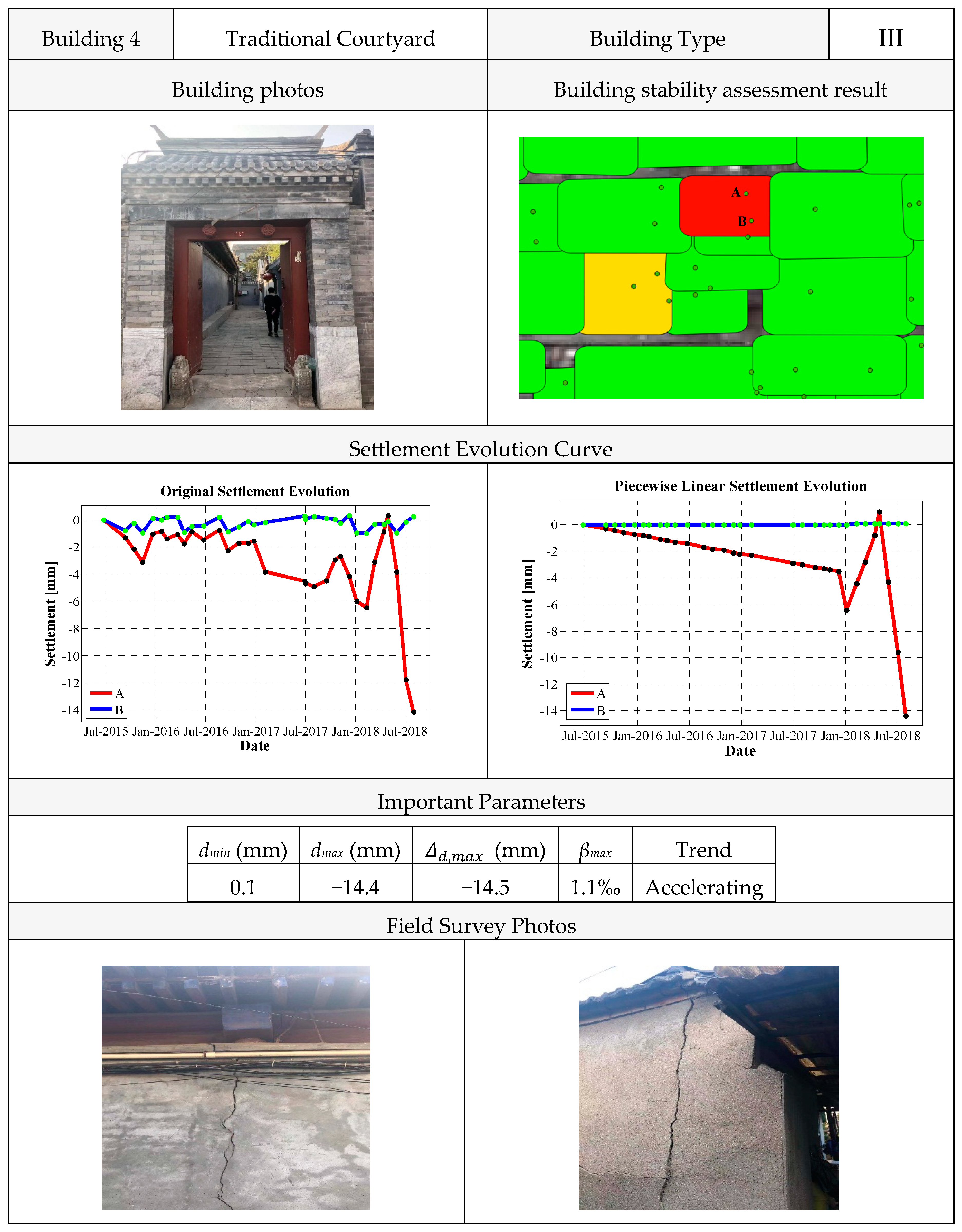
The last example is a traditional courtyard built more than a century ago (see Figure 20). The height of building is about 5 m and its area is about 1000 m². Based on the InSAR results, this building was classified as a type III structure (see Table 1). We calculated a cumulative settlement d_max of about −14.4 mm and the maximum measured differential settlement ${\Delta }_{d,max}$ of about −14.5 mm. The maximum measured angular distortion was then computed to be 1.1‰. Although all the values of the three parameters were not so large, by the analysis of the deformation trend, the settlement rate reached −5 mm/month in the last 3 months of the analysis, showing an acceleration of the phenomenon.

Again, the result of the performed analysis, confirmed by the in situ evidence (significant vertical cracks clearly visible on the wall), detected problems and the necessity to perform a more comprehensive appraisal of this building.

5. Discussion

InSAR techniques applied to high-resolution satellite SAR data are able to extract information over large areas and with unprecedented detail, it also being possible to collect several measurement points over each single building. From one side, this capability opens new opportunities relevant to assessing and monitoring building stability. On the other side, information has to be carefully managed and the interpretation is not intuitive. In fact, satellite InSAR measurements have very peculiar characteristics.

In our approach, the attention can be focused on some “vital points” for each building, and then an analysis of the anomalies in the space and time domains is performed to identify potential risks. In the spatial dimension, a hierarchical clustering is applied to group together the homogeneous PS sets, collapsing them into convergence points. The clustering procedure has the advantage of reducing the noise level and increasing the reliability of the deformation data.

Then, settlement and differential settlement of the observed buildings and structures can be identified with higher precision. In the temporal dimension, by applying a multiple linear regression model, the InSAR displacement measurements are decomposed into two main components: periodic and piecewise linear components. The piecewise linear component is then used to evaluate trend variations (accelerations) in the deformation evolution.

Finally, the joint analysis of the anomalies in the space and time domains substantially improves the stability evaluation capability. The determination of the appropriate thresholds is a difficult task, being related to many factors, such as building structure type, geological conditions, and so on. Therefore, in future developments, we plan to analyze a large number of cases in order to better understand the hidden relationships between deformation measurements and building stability, and be able to provide a stability assessment calibrated and validated with large data statistics.

The procedure proposed in this paper makes it possible to automatically detect and monitor the buildings affected by instability phenomena over large areas by exploiting satellite InSAR datasets. The whole process is automatic and fast. The method has enormous potential, but also some limits. After extensive in situ comparisons and verifications, we could verify that the proposed stability assessment system may underestimate the stability problems of some buildings.

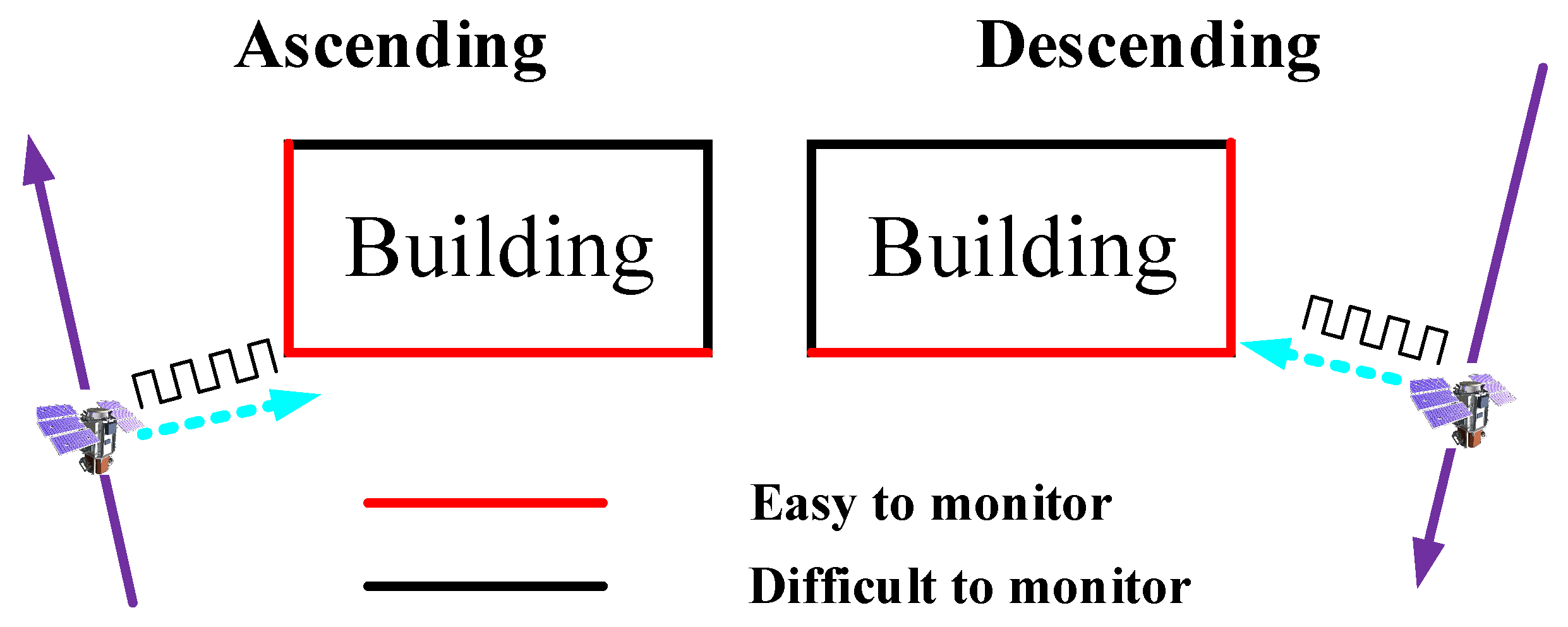
One important limitation is due to the fact that only the building portions facing toward the SAR sensor can be observed. In addition, some buildings or parts of them could suffer from the SAR shadow phenomenon, i.e., they could not be visible from the SAR, for example due to being covered by other tall buildings. As illustrated in Figure 21, due to the side-looking geometry of the SAR sensor, the deformation on the back facets (black lines) of the building cannot be observed. 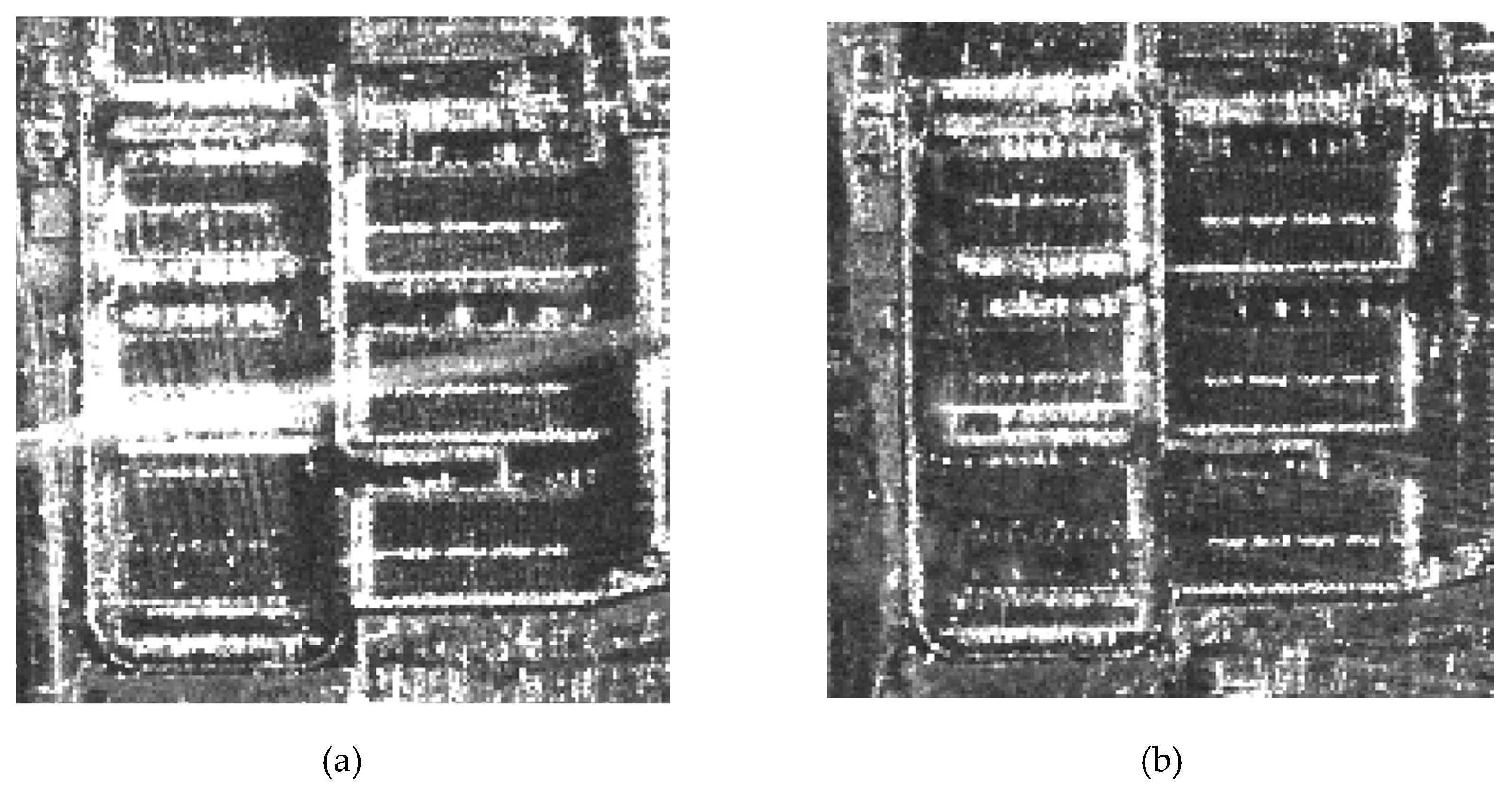In Figure 22, two samples of real amplitude SAR images acquired in ascending and descending geometries, respectively, over an urban area clearly show that the backscattered signal is much stronger on the facets oriented toward the radar. Therefore, we can only obtain incomplete deformation information from the two points of view (ascending and descending orbits) available with the current polar satellites.

Another limitation is that the sampling frequency permitted by the current satellite acquisitions might be insufficient to correctly estimate the target deformation when the phenomenon to be observed is moving too fast.

Moreover, further research is still needed. For example, an effective method to jointly analyze the data obtained by the two satellite acquisition geometries (ascending and descending) should be studied.

However, although satellite InSAR measurements have some limitations (which we hope will be partly overcome by future satellite missions), they provide a unique source of information to observe large areas, in terms of the density, coverage, and temporal sampling of measurements, and can be used to perform a preliminary investigation of the risk associated with the observable buildings. In order to achieve this goal, as much information as possible should be extracted automatically from the measurement data, as we propose with the procedure described in this paper.

6. Conclusions

In this work, a new method is presented for the automatic detection of potential building and infrastructure instabilities from satellite InSAR measurements, by analyzing large cumulative deformations, spatially inhomogeneous settlements, and trends accelerating with time. These anomalous phenomena are particularly critical for the stability of buildings and infrastructures, since damages, or even collapses, are typically related to huge cumulative settlements, differential settlements in different parts of the same structure, or acceleration of the displacement phenomena.

Several examples of building stability assessment in China based on COSMO-SkyMed SAR data processed by means of the PSP InSAR [8] technique have been reported and discussed, demonstrating the ability of the new approach to detect different anomalous deformation features on different buildings. The presented approach takes full advantage of all the information provided by InSAR to increase the probability and reliability of the detection. The in situ survey proved the effectiveness of the new approach.

The method is automatic and makes it possible to analyze a huge amount of data at a relatively low cost. It appears very promising to evaluate the stability or safety of buildings across very large areas and preliminarily analyze the reason for why the displacement occurs. The results obtained from the building stability assessment system would accordingly help the government to open new perspectives for the improvement and optimization of resource planning. Furthermore, based on the InSAR monitoring data, the building appraisal experts could provide more detailed quantitative building risk evaluation.