Assessing Radiometric Correction Approaches for Multi-Spectral UAS Imagery for Horticultural Applications

Abstract

Multi-spectral imagery captured from unmanned aerial systems (UAS) is becoming increasingly popular for the improved monitoring and managing of various horticultural crops. However, for UAS-based data to be used as an industry standard for assessing tree structure and condition as well as production parameters, it is imperative that the appropriate data collection and pre-processing protocols are established to enable multi-temporal comparison. There are several UAS-based radiometric correction methods commonly used for precision agricultural purposes. However, their relative accuracies have not been assessed for data acquired in complex horticultural environments. This study assessed the variations in estimated surface reflectance values of different radiometric corrections applied to multi-spectral UAS imagery acquired in both avocado and banana orchards. We found that inaccurate calibration panel measurements, inaccurate signal-to-reflectance conversion, and high variation in geometry between illumination, surface, and sensor viewing produced significant radiometric variations in at-surface reflectance estimates. Potential solutions to address these limitations included appropriate panel deployment, site-specific sensor calibration, and appropriate bidirectional reflectance distribution function (BRDF) correction. Future UAS-based horticultural crop monitoring can benefit from the proposed solutions to radiometric corrections to ensure they are using comparable image-based maps of multi-temporal biophysical properties.

1. Introduction

There is a direct connection between how much photosynthetic active radiation is absorbed and scattered by plant leaves and their biogeochemical properties. These include: concentrations of photosynthetic pigments in visible bands, along with water and non-photosynthetic pigments in mid-infrared bands, and leaf and canopy structure in near–infrared (NIR) bands [1,2,3,4]. Multi-spectral imagery captured from unmanned aerial systems (UAS) is becoming more commonly used as a technology for monitoring and managing horticultural crops based on such phenomenon [5,6,7,8,9,10]. One of the final products from common commercially available image processing applications is an ortho-rectified mosaic with digital number values [9,10,11]. Although such images are sufficient for some types of classification [4,10,11], the digital numbers only represent the relative brightness range of the ground features and cannot be used to extract consistent information on biophysical properties, derive calibrated vegetation indices or be used to compare multi-temporal datasets. Therefore, the orthomosaic imagery needs to be converted from digital number to normalised at-surface reflectance [4,12].

In past studies, one of the most common ways to correct the imagery from digital numbers to at-surface reflectance has been the simplified empirical approach [8,13,14]. The idea of the empirical method is to identify the relationship between known reflectance targets within the extent of an image to their measured digital number. The best-fit equation produced from this relationship is then used to convert all digital numbers within the image to at-surface reflectance values. A novel correction method to generate an orthomosaiced reflectance image directly without the need for an empirical correction has been developed in recent years for calibrating Parrot Sequoia^® (Parrot Drone SAS, Paris, France) and MicaSense RedEdge^® (MicaSense Inc., Seattle, WA, USA) multi-spectral imagery. The function in the Pix4DMapper software (Pix4D S.A., Lucerne, Switzerland) is called ‘reflectance map’, while a similar function is called ‘calibrate reflectance’ in Agisoft PhotoScan Pro (Agisoft LLC, St. Petersburg, Russia), which uses several photograph parameters to calculate reflectance [15]. In terms of correcting for variations in illumination, software packages such as Agisoft PhotoScan Pro and Pix4DMapper provide ‘colour correction/balancing’ features to implement the image-information-based radiometric block adjustment algorithm. Yet such algorithms only consider the homogeneity of adjacent images’ histogram, regardless of the bidirectional reflectance distribution function (BRDF) effect within a single image. Moreover, studies have also stated that irradiance normalisation and BRDF correction are essential for time-series applications and estimation of biophysical properties [16,17], yet they are not included as features in any commercial UAS processing software packages.

Another issue that has not been addressed in UAS image-bsed radiometric correction is the selection of the most robust normalisation process. Traditionally, various parameters are considered for normalisation when processing satellite images, including solar, topographic, viewing geometries and Sun-Earth distance [4]. As for aerial imagery, the increasing spatial resolution and smaller frame size can cause a higher spectral variance in features information, especially in complex forest environments [18,19,20]. The increasing spatial resolution amplifies observed topographic and BRDF effects within and between image scenes, as the non-uniformity of natural surfaces becomes more obvious at finer scales [19,20]. When coupled with increased variability in measured spectral reflectance observed at smaller pixel sizes, this creates a substantive problem for effective radiometric normalisation. In a highly dynamic platform such as UAS, ineffective normalisation may limit the ability for images of the same area, collected at different times, to be compared.

This study assesses radiometric correction algorithms for UAS imagery provided from commercially available software packages. The applications of BRDF corrections are also investigated. While radiometric correction approaches to satellite and airborne imagery are well established, there is a significant lack of protocols and comparison of methods for radiometrically correcting UAS-based imagery. Our research addresses this gap in knowledge with a specific focus on horticultural environments.

2. Materials and Methods

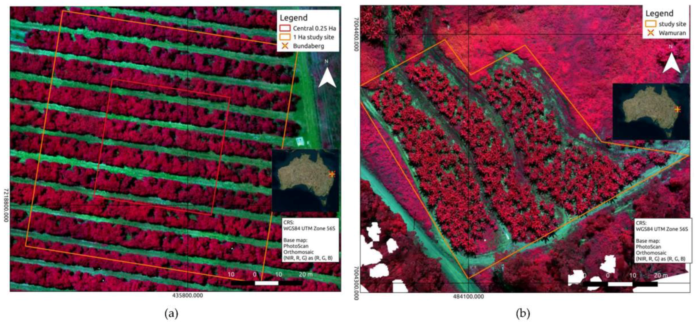
2.1. Study Sites

The two study sites were located in Queensland, Australia. The avocado orchard was located to the south of Bundaberg, which is one of the main avocado producing regions of Australia. The banana plantation was located in Wamuran in the Sunshine Coast hinterland of South East Queensland. The UAV-based focus areas encompassed 1 and 0.5 ha patches of the avocado and banana orchards, respectively (Figure 1). The average elevation for the avocado orchard was around 60 m above sea level, relatively flat terrain with an average slope of 4 degrees downward to the east. The banana plantation was located on a hill slope with an elevation varying from 113 m to 170 m above sea level and an average slope of 21 degrees downward to the north.

2.2. UAS Data Acquisition

Five UAS flight datasets, including three for the avocado orchard and two for the banana orchard, were captured with a Parrot Sequoia multi-spectral camera mounted on a 3DR Solo (3D Robotics, Berkeley, CA, USA) quadcopter under clear sky conditions. The camera acquires imagery in the green (550 nm, 40 nm bandwidth), red (660 nm, 40 nm bandwidth), red edge (735 nm, 10 nm bandwidth), and NIR (790 nm, 40 nm bandwidth) part of the spectrum with its 4.8 × 3.6 mm (1280 × 960 pixels) complementary metal–oxide–semiconductor (CMOS) sensor. The camera is also fitted with an upward-facing irradiance sensor with the same spectral bands. The sensor can measure the arbitrary incoming irradiance for each image frame so that the irradiance measurement can be used for radiometric normalisation.

The image acquisition of the avocado trees was conducted using an established flight grid pattern, which included both along- and across- tree-row flight directions. The first flight was conducted at 75 m above ground level (AGL) on 2 February 2017 between 2:11–2:25 PM (60° solar elevation); the second flight was at 100 m AGL on 3 February 2017 between 12:46–12:59 PM (80° solar elevation); and the third flight was at 50 m AGL on 5 February 2017 between 12:34–12:40 PM (80° solar elevation).

The banana plantation in Wamuran was located in hilly terrain. Therefore, the flight pattern had to follow the direction perpendicular to the slope aspect to ensure safety and data quality. A 1 m digital elevation model (DEM) was used to design the flight plan, to ensure the flight height was maintained at approximately 50 m AGL for each camera waypoint. We used the data from two flights, which were collected between 11:37–11:44 AM and between 12:11–12:17 PM on 4 April 2018. The sun elevation for both flights was approximately 57°. The rest of the flight settings were the same for both the avocado and banana orchard, that is, an 80% sidelap, 1-s image capture interval (>85% forward overlap), and 5 m/s flight speed.

For every dataset, 10 AeroPoints^® (Propeller Aerobotics Pty Ltd., Surry Hills, Australia) were deployed as ground control points (GCPs). The locations of the AeroPoints were recorded for five hours and subsequently post-processed using the Propeller^® network correction based on the nearest base station, located within 26 and 11 km of the Bundaberg and Wamuram study sites, respectively. Eight radiometric calibration panels with greyscales ranging from black to white were deployed, following the method suggested by [8,13]. The reflectance values of the calibration panels were measured with an ASD FieldSpec^® 3 spectrometer (Malvern Panalytical Ltd., Malvern, UK) and ranged from 4% to 92% in all spectral bands, corresponding with the four bands of the Sequoia^® camera (Figure 2). For the banana datasets only, a MicaSense^® calibration panel was used to acquire calibration images for the Parrot Sequoia^® camera.

2.3. Image Pre-Processing

2.3.1. Geometric Correction and Initial Pre-Processing

Agisoft PhotoScan Pro and Pix4DMapper were used to process the multi-spectral UAS data with the addition of in-house Python scripts. For photo alignment, a limit of 10,000 tie points was used with the measured GCPs, derived from the AeroPoint^® centres, imported to geometrically calibrate the images. The geo-referencing root-mean-square errors (RMSE) of the GCPs were 0.07 m, 0.11 m, and 0.02 m for the three avocado datasets, and 0.01 m for both banana datasets, respectively. The overall projection error was 0.6 pixel in all datasets based on the bundle-adjustment error assessment report [21]. The projection errors of tie points were taken into account to eliminate poor-quality points, and a noise filter was also applied to assure the quality of the final products. For the Agisoft PhotoScan Pro, a noise filter was applied during point cloud generation, while for Pix4DMapper the noise filter was applied during the derivation of the digital surface model (DSM). Mild filtering (or sharp smoothening) was used in both workflows to preserve as much detail as possible of the tree crown structure. The final step was to ortho-rectify the image pixels to the DSM and create a mosaic. In Pix4DMapper a vignetting polynomial was used, while for Agisoft PhotoScan Pro, a distance to the surface model was developed for every pixel to simulate the radiant attenuation for vignetting correction [22,23,24]. The two software packages use different projection algorithms to project pixels to the DSM. The orthomosaics from Agisoft PhotoScan look closer to the original images, while the orthomosaics from Pix4DMapper often appeared with a halo effect around the perimeter of tall features (e.g., trees) caused by the ortho-rectification process (Figure 3). By default, Pix4DMapper produces the orthomosaic with colour-balancing enabled, while Agisoft PhotoScan Pro did not have a function to balance brightness until version 1.3 as an optional calibration.

2.3.2. Producing Analysis-Ready Data

At-surface reflectance images were generated for each band for all datasets with four types of correction methods:

• Simplified empirical correction;
• Colour balancing before empirical correction;
• Irradiance normalisation before empirical correction; and
• Sensor-information based calibration.

The empirical correction in methods 1 to 3 was achieved using an in-house Python script to convert digital number (DN) values to at-surface reflectance from the orthomosaic products based on the radiometric calibration panels. This processing workflow produced a total of 144 (4 correction methods × 3 flight patterns × 3 flights × 4 spectral bands) and 32 (4 correction methods × 2 flights × 4 × spectral bands) corrected images from each avocado and banana dataset, respectively. The reason we did not apply irradiance normalisation to the banana data is due to the unstable performance on the avocado data, which will be discussed in the discussion section later. The conceptual workflow of the radiometric correction process is shown in Figure 4.

For method 1, Agisoft PhotoScan Pro was used to produce the orthomosaic with DN values. Its mosaic blending mode calculates weight for each matching pixel and gives the pixel with a projection vector closest to the planar normal vector the highest weight [25]. Blended digital numbers were automatically adjusted based on the camera dark current and sensitivity.

For method 2, we created a colour-balanced orthomosaic with DN values for the avocado data using Pix4DMapper and for the banana data using Agisoft PhotoScan Pro. This was because the colour-balancing feature was not included in the Agisoft PhotoScan Pro software at the time of processing the avocado data and it was preferable to keep the trees in the mosaic as similar to the original images as possible (see Figure 3). Nevertheless, these two software packages use the same algorithm for this task, so similar pixel value patterns were observed. The algorithm generated the new DN value of object point k in image j based on the equation:

$$D{N}_{jk}=a_{re{l}_j}D{N}_{ik}+b_{re{l}_j}$$

(1)

where $D{N}_{jk}$ is the DN value of object point k in adjacent image i; $a_{re{l}_j}$ and $b_{re{l}_j}$ are the applied coefficients to the reference image to ensure that the overlapping images are radiometrically homogeneous.

For method 3, an in-house Python code was used to extract the irradiance measurements recorded by the irradiance sensor and stored in the image metadata, to normalise all raw images using the image with the lowest irradiance as the reference to avoid DN saturation. It adjusted the DN value based on a multiplier coefficient:

$$C_j\left(\lambda \right)=E_{ref}\left(\mathsf{\lambda }\right)/E_j\left(\mathsf{\lambda }\right)$$

(2)

where $E_{ref}\left(\mathsf{\lambda }\right)$ is the irradiance measured in the reference image and $E_j\left(\mathsf{\lambda }\right)$ is the irradiance measured in image j. By multiplying the DN value in image j with $C_j\left(\lambda \right)$, image j can be assigned the same irradiance level as the reference image. Afterwards, the irradiance-normalised images were imported into Agisoft PhotoScan Pro to create the irradiance-normalised orthomosaic.

For method 4, we generated the reflectance image directly based on the equation:

$$\rho =K{f}^2\frac{\left(DN-B\right)G\Gamma }{\left(A\epsilon \gamma +C\right)Count}$$

(3)

where $\rho$ is the reflectance, K is an unknown arbitrary number; f is the camera f-number, ε is the exposure time in seconds, γ is the ISO value; A, B, and C are calibration coefficients which are recorded in the metadata. Count, G, and Γ are parameters of the irradiance sensor, which represent arbitrary irradiance level, gain, and exposure time in seconds respectively. When processing, users can choose whether to enable irradiance input for such calculation. If there is no irradiance measurement or the irradiance measurement input was disabled in the software, the irradiance level is then assumed to be the same across all images. To get K, at least one known reflectance target is required within the image to solve the arbitrariness. Otherwise, the calculated reflectance would be in an arbitrary reflectance without normalisation. This equation can also be applied when there is no irradiance measurement. In this case, it is based on the assumption that the irradiance was a constant and as such can be part of K. If neither importing irradiance measurements nor solving K in Equation (3), the calculated $\rho$ would be surface radiance in an arbitrary unit, which is linearly correlated with ${\mathrm{Wsr}}^{-1}{\mathrm{m}}^{-2}$. This method is relatively novel for UAS image processing but very similar to the conventional way of processing satellite imagery [4]. Equation (3) was applied to convert both avocado and banana datasets to at-surface reflectance. At-surface radiance images were produced for the banana data only. It should be noted that Equation (3) can only be applied to Parrot Sequoia products because different sensors use different conversion equations.

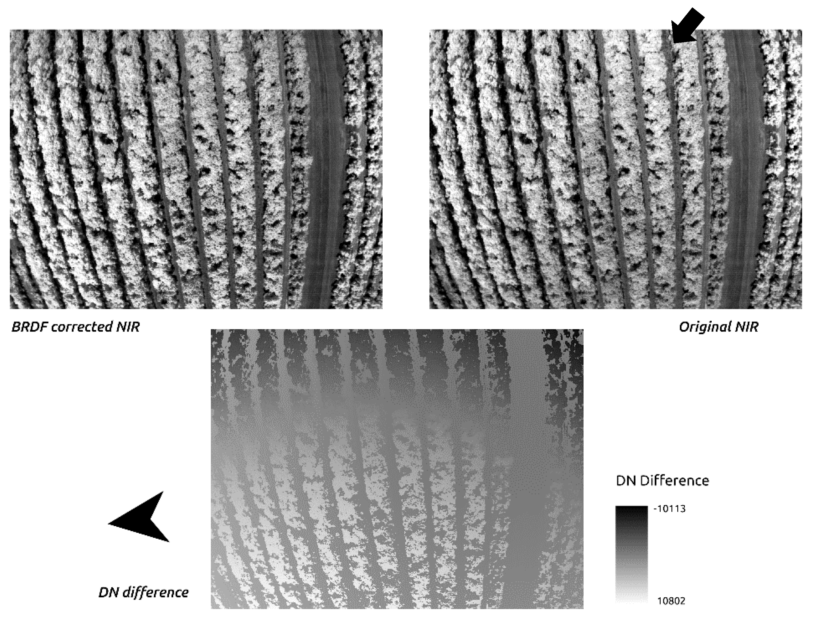
2.3.3. Correcting for Solar and Viewing Geometries Within and Between Images—Bidirectional Reflectance Distribution Function (BRDF)

Previous studies suggest that BRDF correction increases the brightness homogeneity of the mosaiced images for crop fields [16,17]. To address this, we implemented a BRDF correction using the Walthal model [26] with an in-house Python script as a plugin of Agisoft PhotoScan Pro. For each pixel, it is assumed we can back-calculate their spatial location accurately as well as their projection on the earth after optimising camera positions and orientations with the aid of GCPs. Based on the known solar ephemeris, we can calculate the solar zenith and azimuth angles at a specific date and time for every pixel. Sensor view zenith and azimuth angles were calculated using the projection vectors from the camera centre to each pixel, then transform the vectors from the camera coordinates to the world coordinate system. With the known illumination and viewing angles, we can then use the parameters to solve a Walthal BRDF model using tie points as multiple observations. The Walthal BRDF model is described as:

$$r=a{\theta }_v^2+b{\theta }_v\cos \left({\phi }_v-{\phi }_s\right)+c$$

(4)

where r is the reflectance, ${\theta }_v$ is the viewing zenith angle, ${\phi }_v$ is the viewing azimuth angle, ${\phi }_s$ is the sun azimuth angle; and a, b, and c are the coefficients of the multivariate linear regression. We can calculate the nadir reflectance for the tie points by calculating the c value. In a horticultural environment, it is assumed there are usually two features on the ground: soil and vegetation. Therefore, we solved the Gaussian mixture model for each image and predicted which feature each pixel belonged to, based on its DN value. The linear regression for each feature in each image based on the tie points’ BRDF models was then calculated. By predicting which feature each pixel belonged to, a respective linear regression was applied to calculate the nadir reflectance for every pixel. For the avocado data, the BRDF correction was only applied to the generated orthomosaic with colour-balancing (method 2), following the recommendation of previously reported studies [16,17]. However, the BRDF correction algorithm was applied to the banana data with the sensor-information-based calibration (method 4), to explore a workflow which is similar to method applied to satellite imagery for obtaining at-surface reflectance.

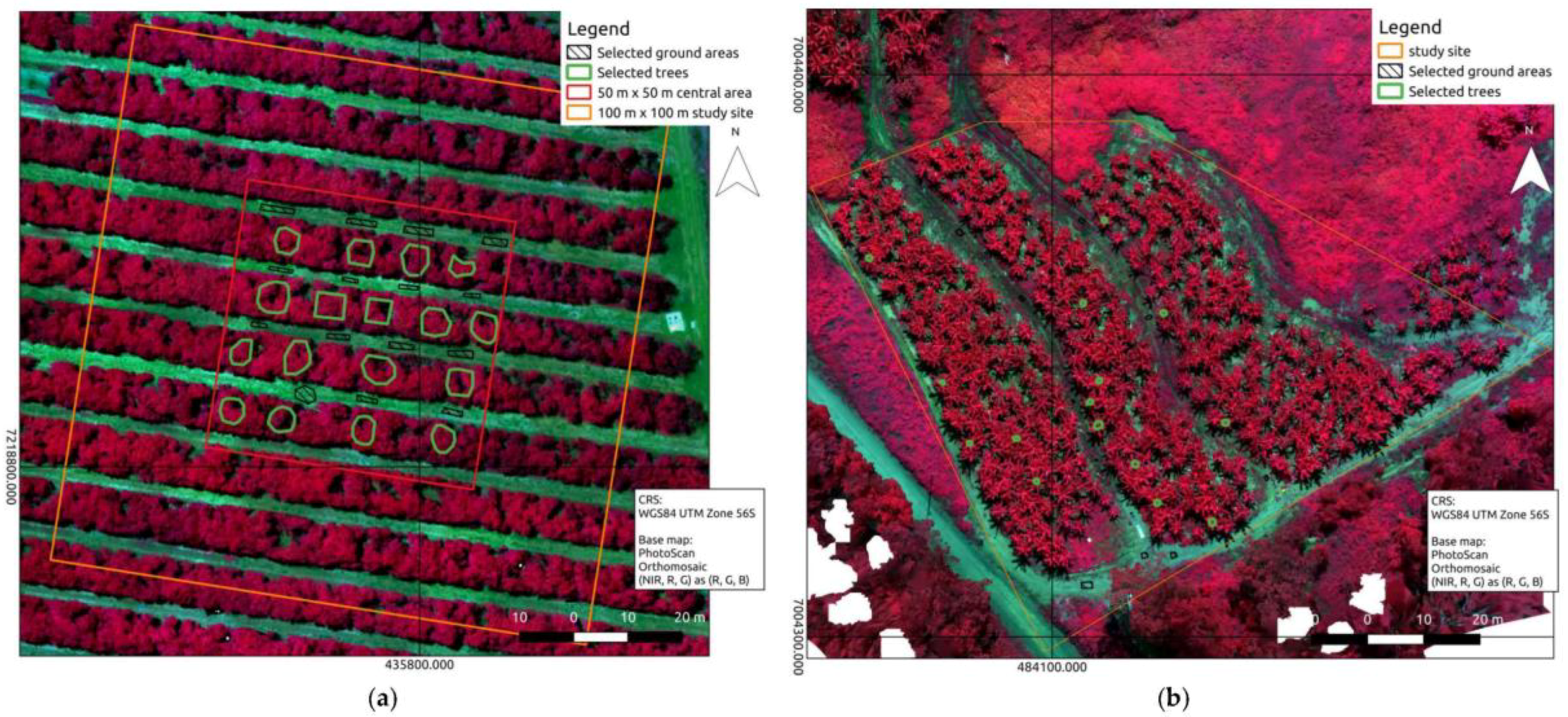
2.4. Assessment of Canopy Reflectance Consistency

If it is possible to correct both internal and external errors due to canopy geometry and image orientation, then it should be possible to achieve similar results from the measurements which are conducted at the same time for the same features [1,19,27,28]. In other words, if a correction algorithm works properly, the corrected images from the temporally near-coincident datasets should provide consistent surface reflectance regardless of the variation in acquisition parameters.

It was difficult to guarantee that the distribution of pixel values would be similar in the same area from different datasets, due to the variations in observation perspectives among different flights caused by differences in flying height, speed and flying pattern. However, we can still compare the similarity of the datasets in terms of calibrated pixel values using methods relying on simple statistical values such as box-and-whisker comparison. We compared the medians and interquartile range (IRQ) between two datasets to determine the likelihood of difference at the scale of objects, that is, individual trees and patches of bare ground. If the two datasets did not have overlapping IRQs, we can confidently say that the two datasets are significantly different. If the IRQs are overlapping, then we can use the fraction of difference between medians (DBM) over overall visible spread (OVS) to determine whether there is a difference between two datasets. As Wild, et al. [29] suggested, the critical fraction to identify the difference of DBM/OVS are stated as follow:

5.

For a sample size of 30, if this fraction is over 33%, there tends to be a difference.

6.

For a sample size of 100, if this fraction is over 20%, there tends to be a difference.

7.

For a sample size of 1000, if this fraction is over 10%, there tends to be a difference.

In this case, the sample size is the pixel counts of the selected objects in the images. Based on the sample size and fraction values provided by [29], the critical fraction for the sample size between these numbers can be derived using the exponential relationship between the fraction criterion and the natural logarithm of the sample size as:

$$\mathrm{critical}\mathrm{fraction}=2.6104\times {(\ln \left(sample size\right))}^{-1.686}$$

(5)

This equation can help to determine the critical fraction for samples which have less than 1000 samples. Once the sample size reaches 1000, 10% is enough to determine if there tends to be a difference between two datasets. If the calculated DBM/OVS fraction had not exceeded the respective critical fraction, we concluded that there was no significant difference between the different input data. Thus, the estimated reflectance for selected feature was consistent between the datasets.

For the avocado and banana image datasets, the areas and number of sites sampled were chosen purposely, to cover variability in the trees, but also to be logistically feasible within our resources and time. The sample datasets will contain some bias, but it was not possible to obtain an exhaustive and statistically sound data set within our time constraints. For the avocado trees, we visually delineated image areas in the inner tree crowns for 17 purposely selected trees. In association with these trees, image areas of 15 flat and weed-free ground areas, were also purposely selected. For the banana data, image areas of 15 trees and 10 ground areas were selected for the comparison (Figure 5). The delineated areas were saved as ESRI shapefiles and then batch-processed using an in-house Python script to derive zonal statistics of the delineated areas from corrected images, including median, the first quartile, the third quartile, minimum extreme, and maximum extreme. Such statistical attributes were extracted to Microsoft Excel files and compared between the same sampled feature from temporal near-coincident images which were corrected with the same correction method. The percentage of consistent results divided by total inputs was defined as the consistency rate in our study and used as an indicator of the robustness of each correction method.

3. Results

In this section, we present the results of the calibrated reflectance consistency assessment with object-based box-and-whisker comparison for the avocado images. The box-and-whisker comparison results for the banana images will subsequently be presented. It should be highlighted that the analysis results in this section show the consistency of the calibrated reflectance rather than the absolute accuracy compared to other spectral measurements.

3.1. Reflectance Consistency Assessment of Avocado Imagery

Figure 6 shows the consistency rate of the calibrated reflectance for the 17 selected tree canopies and 15 selected ground patches. Detailed comparison for tree canopies and ground areas can be found in

Table A1. Reflectance consistency percentages of tree canopies between different flight patterns in dataset 1.

Correction Method	Band	Along vs. Cross	Along vs. Grid	Cross vs. Grid
Empirical correction	Green	41.2%	11.8%	0%
	Red	0%	0%	0%
	Red edge	58.8%	76.5%	76.5%
	NIR	82.4%	94.1%	70.6%
Colour balancing + Empirical correction	Green	58.8%	94.1%	88.2%
	Red	23.5%	88.2%	41.2%
	Red edge	29.4%	88.2%	70.6%
	NIR	47.1%	76.5%	82.4%
Irradiance normalisation + Empirical correction	Green	0%	47.1%	0%
	Red	0%	0%	0%
	Red edge	76.5%	70.6%	82.4%
	NIR	82.4%	94.1%	88.2%
Sensor-information-based calibration	Green	47.1%	100%	82.4%
	Red	0%	52.9%	0%
	Red edge	47.1%	0%	0%
	NIR	0%	88.2%	0%

,

Table A2. Reflectance consistency percentages of tree canopies between different flight patterns in dataset 2.

Correction Method	Band	Along vs. Cross	Along vs. Grid	Cross vs. Grid
Empirical correction	Green	0%	58.8%	0%
	Red	0%	11.8%	0%
	Red edge	64.7%	47.1%	88.2%
	NIR	64.7%	70.6%	76.5%
Colour balancing + Empirical correction	Green	11.8%	0%	0%
	Red	17.6%	0%	0%
	Red edge	47.1%	17.6%	52.9%
	NIR	11.8%	82.4%	11.8%
Irradiance normalisation + Empirical correction	Green	47.1%	58.8%	76.5%
	Red	23.5%	5.9%	5.9%
	Red edge	47.1%	70.6%	94.1%
	NIR	52.3%	82.4%	23.5%
Sensor-information-based calibration	Green	0%	0%	0%
	Red	0%	23.5%	0%
	Red edge	0%	100%	0%
	NIR	0%	88.2%	0%

and

Table A3. Reflectance consistency percentages of tree canopies between different flight patterns in dataset 3.

Correction Method	Band	Along vs. Cross	Along vs. Grid	Cross vs. Grid
Empirical correction	Green	0%	5.9%	0%
	Red	0%	58.8%	0%
	Red edge	5.9%	35.3%	5.9%
	NIR	5.9%	82.4%	0%
Colour balancing + Empirical correction	Green	0%	52.9%	0%
	Red	0%	17.6%	0%
	Red edge	23.5%	29.4%	17.6%
	NIR	0%	76.5%	0%
Irradiance normalisation + Empirical correction	Green	0%	0%	0%
	Red	0%	52.9%	0%
	Red edge	29.4%	52.9%	70.6%
	NIR	0%	88.2%	0%
Sensor-information-based calibration	Green	0%	5.9%	0%
	Red	0%	0%	0%
	Red edge	0%	88.2%	0%
	NIR	0%	64.7%	0%

and

Table A4. Reflectance consistency percentages of ground areas between different flight patterns in dataset 1.

Correction Method	Band	Along vs. Cross	Along vs. Grid	Cross vs. Grid
Empirical correction	Green	33.3%	0%	0%
	Red	0%	0%	0%
	Red edge	33.3%	60%	40%
	NIR	40%	66.6%	60%
Colour balancing + Empirical correction	Green	0%	0%	6.7%
	Red	13.3%	13.3%	20%
	Red edge	20%	40%	33.3%
	NIR	40%	73.3%	46.7%
Irradiance normalisation + Empirical correction	Green	33.3%	20%	0%
	Red	0%	6.7%	0%
	Red edge	26.7%	40%	26.7%
	NIR	13.3%	53.3%	33.3%
Sensor-information-based calibration	Green	40%	73.3%	20%
	Red	0%	53.3%	0%
	Red edge	6.7%	0%	0%
	NIR	13.3%	60%	6.7%

,

Table A5. Reflectance consistency percentages of ground areas between different flight patterns in dataset 2.

Correction Method	Band	Along vs. Cross	Along vs Grid	Cross vs. Grid
Empirical correction	Green	26.7%	6.7%	26.7%
	Red	6.7%	6.7%	6.7%
	Red edge	66.7%	26.7%	40%
	NIR	13.3%	6.7%	60%
Colour balancing + Empirical correction	Green	0%	0%	0%
	Red	0%	6.7%	6.7%
	Red edge	33.3%	6.7%	26.7%
	NIR	26.7%	40%	26.7%
Irradiance normalisation + Empirical correction	Green	0%	26.7%	40%
	Red	0%	0%	20%
	Red edge	60%	40%	20%
	NIR	40%	46.7%	46.7%
Sensor-information-based calibration	Green	6.7%	0%	0%
	Red	13.3%	40%	6.7%
	Red edge	6.7%	53.3%	0%
	NIR	6.7%	40%	0%

and

Table A6. Reflectance consistency percentages of ground areas between different flight patterns in dataset 3.

Correction Method	Band	Along vs. Cross	Along vs. Grid	Cross vs. Grid
Empirical correction	Green	0%	0%	0%
	Red	0%	13.3%	0%
	Red edge	0%	40%	6.7%
	NIR	0%	93.3%	0%
Colour balancing + Empirical correction	Green	0%	20%	0%
	Red	20%	0%	0%
	Red edge	26.7%	6.7%	26.7%
	NIR	0%	46.7%	0%
Irradiance normalisation + Empirical correction	Green	0%	0%	0%
	Red	6.7%	6.7%	0%
	Red edge	40%	40%	33.3%
	NIR	0%	60%	0%
Sensor-information-based calibration	Green	0%	20%	0%
	Red	0%	0%	0%
	Red edge	0%	73.3%	0%
	NIR	0%	6.7%	0%

respectively. From Figure 6, we can tell that the reflectance consistency was much better for the canopy areas than the ground areas. Datasets 1, 2, and 3 had above ground flight altitudes of 75 m, 100 m, and 50 m, and solar elevation of approximately 60°, 80°, and 80° respectively. As mentioned before, we compared the sub-datasets which were the data with different flight patterns from the same flight. Therefore, since the tree canopy biophysical conditions did not change much during one flight, a high consistency percentage across all flight patterns was expected if a correction method was optimal. It is noted that the consistency rates of the red edge and NIR bands are mostly moderate and higher than the green and red bands, especially using the empirical-correction-based methods. However, it seems that no correction method provided an overall high consistency percentage for all bands in all datasets in this presented experiment. No correction method provided consistently corrected reflectance values even for the canopy areas for dataset 3. The performance of colour-balancing and irradiance normalisation was not stable. Both of them increased the consistency rate in some of the datasets while decreased in others.

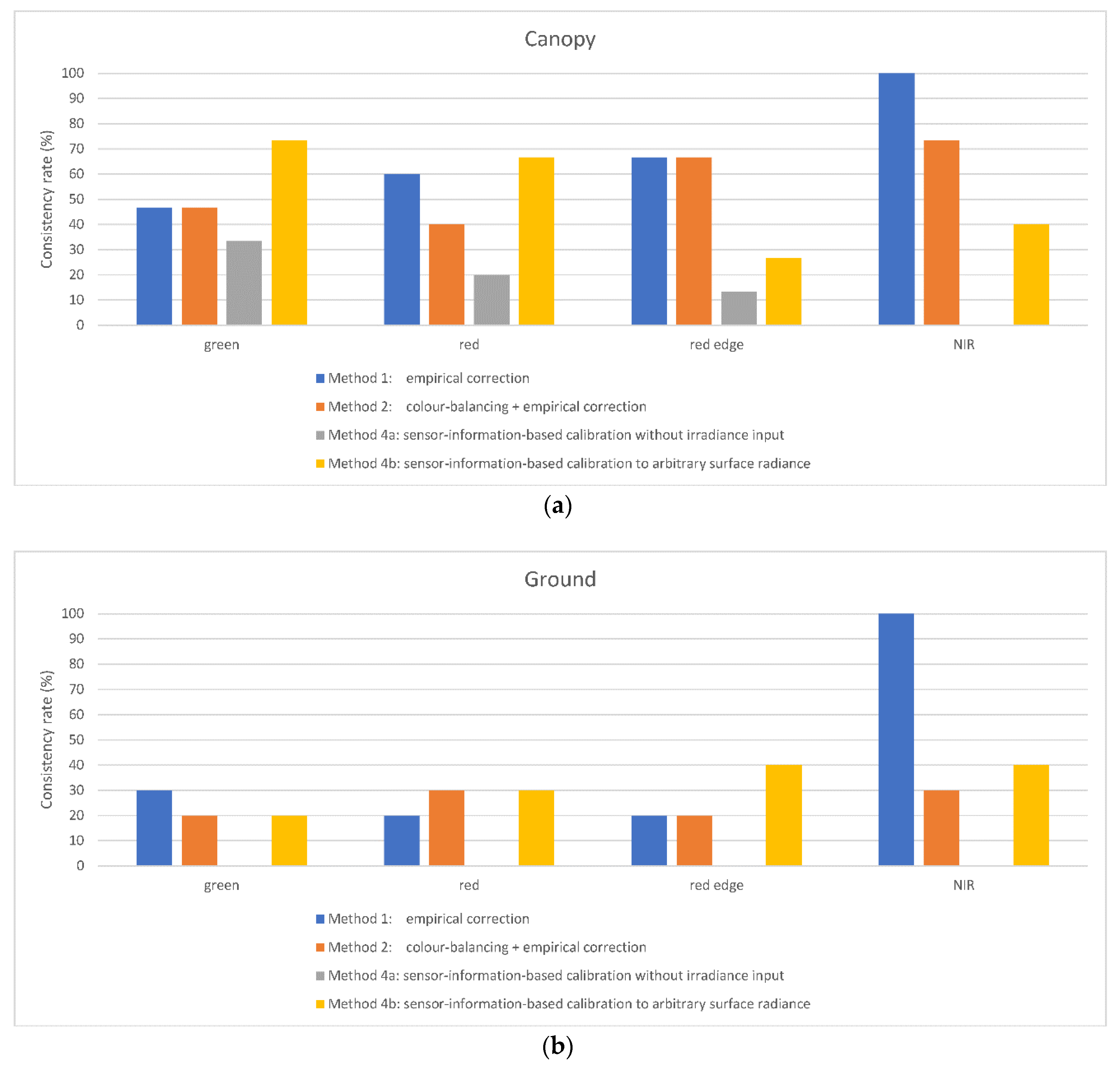
3.2. Correction Consistency Assessment of Banana Imagery

Figure 7 shows the consistency rate of the radiometrically calibrated values between two temporally close datasets for the 15 selected tree canopies and 10 selected ground patches. Detailed information can be found in

Table A7. Consistency assessment results from the box-and-whisker plot comparison between two temporally close flights.

Correction Method	Band	Canopies	Ground
Empirical correction	Green	46.7%	30%
	Red	60%	20%
	Red edge	66.7%	20%
	NIR	100%	100%
Colour balancing + Empirical correction	Green	46.7%	20%
	Red	40%	30%
	Red edge	66.7%	20%
	NIR	73.3%	30%
Sensor-information-based calibrated surface reflectance	Green	33.3%	0%
	Red	20%	0%
	Red edge	13.3%	0%
	NIR	0%	0%
Sensor-information-based calibrated arbitrary surface radiance	Green	73.3%	20%
	Red	66.7%	30%
	Red edge	26.7%	40%
	NIR	40%	40%

. From Figure 7, we can tell that the calibrated values of canopies were more consistent than those for the ground areas, except for the NIR band using the simplified empirical correction. The consistency rates for the canopies in the red edge and NIR bands were generally higher than those for the green and red bands when the images were corrected with the empirical-correction-based method. It is noted that although the reflectance consistency rate was poor in the sensor-information-based calibration, the calibrated arbitrary radiance provided the highest consistency for the green and red bands.

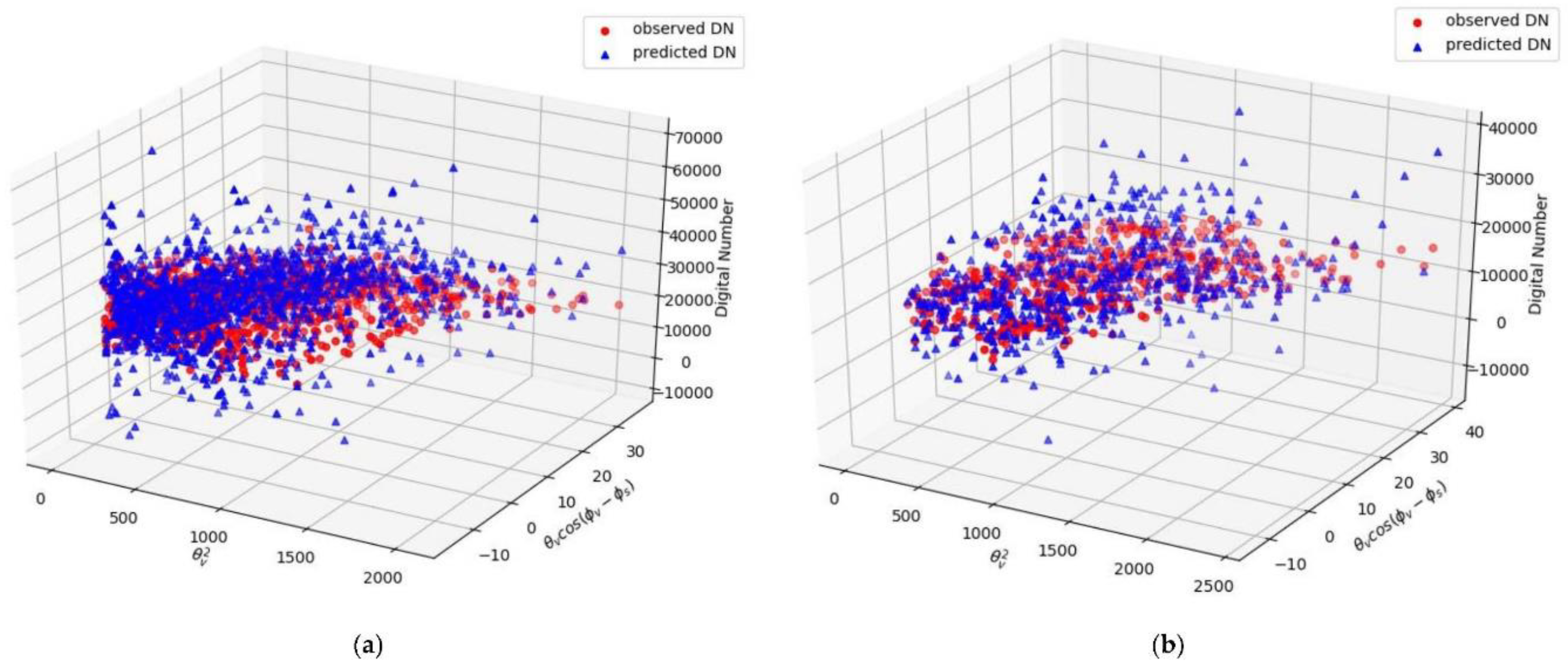
3.3. BRDF Correction Consistency Assessment

Figure 8 shows the estimated BRDF models for both canopy and ground features for an avocado orchard image in the NIR band. Both prediction models and Figure 9 show that most of the DN changes, where BRDF corrections were largest, occurred in the canopy areas. We analysed both single image brightness homogeneity and surface reflectance consistency to assess whether the proposed BRDF correction worked properly.

We used an image which contained mostly ground features and calculated the DN mean for every row and column. The covariance of rows and columns between the original image and corrected image were then compared to assess the single image brightness homogeneity for the avocado datasets. The larger the covariance was, the larger the DN values varied through the whole image. Results show that the covariance of the original image was 4,409,616 DN, whereas the covariance of the BRDF corrected image was 3,864,839 DN, which means the overall spread of DN distribution became smaller after BRDF correction. We also used images where the calibration panels were in different locations to compare the DN values difference. The black panel in the original images had a DN difference up to 6000 higher when the panel was near the image edge rather than at the centre, where the difference was reduced to around 1000 in the BRDF corrected images. These assessments were evidence that the proposed algorithm increased the brightness homogeneity. Increasing brightness homogeneity for the same features from different images can reduce brightness variation between similar features. From Figure 9, we can tell that the hot spots in some of the original images of the avocado orchard were eliminated after BRDF correction.

Table 1. Reflectance consistency percentages between different flight patterns in dataset 2.

Correction Method	Band	Along vs. Cross	Along vs. Grid	Cross vs. Grid
BRDF + Colour balancing + Empirical correction on canopies	Green	0% (same)	0% (same)	5.9% (better)
	Red	0% (same)	0% (same)	0% (same)
	Red edge	52.9% (better)	88.2% (better)	64.7% (better)
	NIR	41.2% (better)	17.6% (worse)	64.7% (better)
BRDF + Colour balancing + Empirical correction on ground	Green	0% (same)	0% (same)	6.7% (better)
	Red	0% (same)	0% (worse)	26.7% (better)
	Red edge	0% (worse)	26.7% (better)	0% (worse)
	NIR	6.7% (worse)	6.7% (worse)	46.7% (better)

shows the results of the box-and-whisker plot comparison for assessing reflectance consistency between different flight patterns. The proposed BRDF correction did not improve the performance in the green and red bands. Compared to the result of colour balancing before the empirical correction in Table A2 and Table A5, the overall consistency increased a little bit in the red edge and NIR bands for canopies, although the difference was not significant. The consistency became even worse for the ground areas.

The results of the BRDF correction with sensor-information-based calibration for the banana datasets did not provide robust solutions either (

Table 2. Consistency assessment results for banana from box-and-whisker comparison between two temporally close flights.

Correction Method	Band	Canopies	Ground
BRDF + Sensor-information-based calibrated surface reflectance	Green	46.7% (better)	10% (better)
	Red	26.7% (better)	0% (same)
	Red edge	26.7% (better)	0% (same)
	NIR	33.3% (better)	0% (same)
BRDF + Sensor-information-based calibrated arbitrary surface radiance	Green	33.3% (worse)	10% (worse)
	Red	33.3% (worse)	40% (better)
	Red edge	53.3% (better)	0% (worse)
	NIR	20% (worse)	20% (worse)

). Although the consistency rate of at-surface reflectance increased by a maximum of 33% in NIR band, the consistency of the calibrated at-surface radiance dropped significantly in the green and red bands compared to the results in Table A7.

To sum up, we found that for the avocado datasets, none of the proposed corrections provided consistent at-surface reflectance in the green and red bands. The empirical corrections provided moderate consistency rates in the red edge and NIR bands when the data was acquired above 75 m AGL. There is no evidence to prove that colour-balancing and on-board irradiance normalisation provided robust improvements in consistency rates. However, the proposed BRDF correction somehow improved consistency rates in the red edge and NIR bands for the canopy areas compared to the colour-balancing correction. This result is an important finding in terms of the use of UAS, particularly the NIR band for mapping variability in tree health. High NIR reflectance is synonymous with high tree vigour [30,31], and as such, using these image layers where high NIR reflectance is the result of a BRDF effect as opposed to actual tree variability may lead to incorrect assessment of crop condition and management decisions. For the banana datasets, we found that the empirical correction provided moderate consistency rates in the green and red bands even though the data was acquired at 50 m AGL. The consistency rates in the red edge and NIR bands were still higher, consistent with the observations for the avocado datasets. The sensor-information-based calibrated at-surface reflectance had the worst consistency rates in all bands. Nevertheless, the sensor-information-based calibrated arbitrary at-surface radiance showed the best consistency rates in the green and red bands. A brief performance comparison of the proposed methods can be found in

Table 3. A simplified comparison table of the proposed correction methods. G, R, RE, and NIR are green, red, red edge, and NIR bands respectively. X means the method doesn’t work well; V means the method works well; Δ means the results are unstable; O means the results are moderately consistent.

Correction Method	Avocado Datasets				Banana Datasets
	G	R	RE	NIR	G	R	RE	NIR
Simplified empirical correction	X	X	V	V	O	O	V	V
Colour-balancing + empirical correction	X	X	Δ	Δ	O	O	V	V
Irradiance normalisation + empirical correction	X	X	Δ	Δ
Sensor-information-based calibrated reflectance	X	X	X	X	X	X	X	X
Sensor-information-based calibrated radiance					V	V	X	O
Remarks	None of them works when flight altitude is 50 m

.

4. Discussion

4.1. The Influences of Flight Altitude and Image Scale

There are several factors which affect the reflectance of tree canopies, such as viewed area, canopy geometry, terrain, and the viewing geometry between the ground surface, sensor, and the Sun [19]. As the spatial resolution increases, so does the variance of observed reflectance [19]. In addition, increasing spatial resolution in UAS imagery comes with lower flight altitude, which also means that each camera frame covers a smaller area. When creating orthomosaics for the same area with smaller image frames, higher variation in the illumination conditions and solar-viewing geometry will occur [12,16,17,19]. Therefore, the cause of the reflectance inconsistency in dataset 3 of the avocado orchard may be due to these two factors. Besides, when pre-processing satellite images, the topographic effect caused by terrain is much more severe than individual features in the scene so that the canopy geometry variation can usually be simplified by simple physical models [32]. However, when the spatial resolution increases, the canopy geometry starts contributing to the variation in reflectance which is no longer negligible.

Moreover, it is well-known that the reflection properties of natural materials are usually scale-dependent [33]. For very high spatial resolution imagery such as that acquired by a UAS, the BRDF effect becomes more serious because of increasing Sun-surface-view geometry variation [19]. For correcting topographic effects for large-scale images, the Lambertian assumption is applied to most of the natural surfaces [33]. However, many studies have suggested that the BRDF models for natural surfaces are more sophisticated instead of being Lambertian [34,35,36,37]. Meanwhile, the diffusive illumination from the environment may affect the observed reflectance as well [33,38]. Such scattering from surroundings is easier to observe from the fine-scale measurement [38]. This factor may be the cause of the inconsistent reflectance we found in our ground samples and some of the tree canopies. In a horticultural environment, trees cover the majority of a scene, and ground areas are surrounded by trees. Therefore, we suspect that the higher possibility of diffusive light influenced the radiance the camera acquired, especially in the ground areas.

4.2. The Influence of Canopy Geometric Complexity on Reflectance Consistency

As mentioned above, the reflectance variation caused by canopy geometry becomes significant as the spatial resolution increases. This effect can be observed in the avocado datasets. Avocado datasets 2 and 3 had almost the same acquisition conditions, except for the flight altitude. Dataset 2 had a flight altitude of 100 m, which resulted in a 9.86 cm ground sample distance (GSD), whereas dataset 3 at a flight altitude of 50 m had a GSD of 4.74 cm. At such a high spatial resolution, we suspect that the effect of directional reflectance caused by leaf angle variation also started to contribute to radiometric distortion due to the reflection angle non-uniformity. In addition, such effect was more serious for the avocado orchard than for the banana plantation because the complexity of avocado tree crowns is much higher. The avocado dataset 3 had the same flight altitude as the banana datasets. However, there was no reflectance consistency in avocado dataset 3 while there was still some consistency observed in the banana datasets.

4.3. The Limitation of Simplified Empirical Correction

Studies have observed that the Parrot Sequoia multi-spectral camera has different sensitivity in different bands, and the maximum detectable reflectance for green and red bands is around 40% [39]. The saturation problem in the green and red bands reduces the effectiveness of empirical correction because it reduces the samples for calculating the linear regression. Moreover, the diffusive radiant flux in the horticultural environment may also cause the observed albedo of the calibration panels in the UAS images to be inaccurate, especially if the panels were deployed in a tree-surrounded area. Since the green and red bands are more sensitive, we suspect that the scattering of green and red radiant flux from the environment influenced the albedo measurement of the panels more seriously. Such characteristics can explain why the empirical correction always resulted in worse consistency in the green and red bands. Besides, the bidirectional reflectance phenomenon was also observed on the panels (see Section 3.3). Perfectly Lambertian surface materials are expensive so we used a more cost-effective alternative, which was proposed by Wang and Myint [13]. However, brightness variation in panels was still observed in some individual images. Except for the possible diffusive flux influence, some of the brightness difference may be caused by backscatter as well.

In addition, the canopy geometric complexity of avocado trees also caused some problems when applying empirical corrections. The calibrated reflectance was very often negative in the green and red bands in the avocado data when using the empirical correction, but such a negative reflectance problem was absent in the banana data using the same correction. We suspect that the complex canopy geometry caused many shaded leaves within tree crowns so that those shaded leaves obtained negative reflectance values after applying the empirical correction based on the panels. Besides, as previously mentioned, diffusive green and red radiant flux may increase the measured albedo from the panels, creating a false relationship between pixel DN and at-surface reflectance. Setting the linear regression with a 0 interception could solve the negative values problem. However, this is not practical since the minimum DN value depends on the black current of the camera instead of zero. The negative reflectance will cause problems when deriving vegetation indices from the reflectance data. The solution is subtracting the minimum value which was found in the canopy areas (equivalent to adding the value which has the maximum magnitude in the negative domain) from the calibrated reflectance image, as long as the reflectance still matches the spectral signature of vegetation.

4.4. UAS Based Irradiance Measurements

We also noticed that the irradiance measurements with the Sequoia^® irradiance sensor had directional variation. In avocado dataset 1, the solar elevation was around 60°, and the flight direction was along-row, approximately aligned with the direction of the Sun. Comparing this with the coincident dataset, which was flown perpendicular to the Sun direction, the recorded irradiance measurements from adjacent images appeared with a 30% difference in its arbitrary irradiance unit, which is homogeneous to ${\mathrm{Wm}}^{-2}$. Such differences may be the cause of unstable correction performance (see Table 3). Most of the modern onboard UAS irradiance sensors are equipped with a cosine corrector, which was proved to increase the accuracy [40]. The lack of a cosine corrector for the Sequoia irradiance sensor may prevent the measured irradiance from being direction independent. This is why we did not apply the irradiance measurements for the radiometric correction and the sensor-information-based calibration for the banana datasets.

4.5. Proposed BRDF Correction

From Table 1, we can tell that the proposed BRDF correction did not improve the reflectance consistency. Part of the reason may be due to the limitation of the empirical correction we mentioned in Section 4.3. However, from Table 2, we can tell that even without applying the empirical correction, the BRDF correction did not provide a robust solution for consistent measurements. Such inconsistency may be caused by non-uniform leaf inclination angle, which is proved to impact the BRDF models [26,35]. Besides, some studies also suggested that the topographic effect on the BRDF models need to be addressed [19,33]. As we discussed in Section 4.1, with very fine-scale UAS imagery, the non-uniform reflection properties caused by solar-surface-viewing geometry variation starts to affect the observation. Therefore, instead of only addressing the solar-viewing geometry, as with the proposed BRDF correction algorithm, the surface topography also needs to be considered for solving solar-surface-viewing geometry variation.

Another problem in our proposed algorithm is that solving the Gaussian mixture model of the pixel value distribution did not provide a good prediction to the objects in the images. Although there were usually two types of features in the scenes, there were many pixels in the canopies belonging to shaded leaves that were classified as ground features, and some pixels of the ground features which had hot spots that were classified as canopies. The wrong prediction of features resulted in the inappropriate linear regression being applied to those pixels. Consequently, such corrected images were very likely to make the correction more inconsistent. Since object detection using machine learning in UAS imagery has significantly progressed [41,42,43], we believe that this technology can possibly provide a robust solution to object detection. The correct object detection can help to solve the BRDF problem by providing the correct model to respective objects in the images. An accurate object detection method can also help us to build empirical BRDF models for specific features in the images with enough input data. We believe that this will be a convenient way to deal with the BRDF problem.

4.6. Potential of Sensor-Information-Based Calibration

Although the sensor-information-based calibration to at-surface reflectance with panel input did not work very well (Figure 7), the arbitrary at-surface radiance from such calibration provided the best consistency in the green and red bands. The reason that the calibrated at-surface reflectance was not consistent may be due to insufficient data to correlate the radiance with reflectance. This method only relies on one reflectance target to solve the arbitrariness instead of creating a linear relationship over a range of reflectance values. Additionally, this calibration heavily relies on the coefficients provided by the manufacturers (Equation (3)). This characteristic can explain why the at-surface radiance consistency rates in the red edge and NIR bands were not as high as the green and red bands because the coefficients recorded in the firmware may not have been as accurate. The behaviour of how captured radiance is converted to DN may also change after a firmware update. Therefore, camera manufacturers should pay careful attention to identify the physical variables collected to calibrate the sensor, to make sure the energy-to-signal conversion behaviour works as expected [44,45]. Moreover, with the in-situ radiance measurement, camera end users could possibly calculate the conversion equation themselves to fit their needs in the local environments [44]. Once we can figure out accurate calibration parameters for a specific camera to get accurate surface radiance in ${\mathrm{Wsr}}^{-1}{\mathrm{m}}^{-2}$, it is possible to use either ground or onboard irradiance sensors to measure the irradiance in ${\mathrm{Wm}}^{-2}$ to calculate accurate surface reflectance.

5. Conclusions

Our results show that the bidirectional reflectance distribution function (BRDF) is an essential factor, which needs to be taken into account to reduce brightness variations due to illumination and sensor geometries in UAS images. As discussed in Section 4.1 and Section 4.5, the fine-spatial scale characteristic of UAS imagery causes more serious BRDF effect. Past studies suggest that using the Walthal BRDF model will resolve the solar-viewing geometry variation [17]. However, in a more complex environment like orchards or even forest, the topography should also be considered to resolve the solar-surface-viewing geometry variation instead [33]. With enough input data, we can even build empirical BRDF models for features of interest and apply the respective models to different features in the images with the aid of object detection. Accurate BRDF model application should enable effective BRDF correction, which allows accurately mosaicking UAS images to provide more accurate analysis ready data for mapping and monitoring environmental changes.

The simplified empirical correction worked to some degree. Although the simplified empirical correction has proved to provide some good results in precision agricultural applications [12,14], for measuring trees with complex canopy geometry, it is suggested not to acquire UAS imagery below a specific height because the smaller frame size and higher spatial resolution can increase the variation of solar-surface-viewing geometry. Some studies also suggested that flying the UAS at around 80 m AGL is the optimal protocol for measuring trees [8,46], which is very close to the height threshold we found for the avocado datasets. Besides, the surrounding environment of the calibration panels plays an important role to provide accurate reference. As we discussed in Section 4.3, it should be as open and flat as possible to avoid diffusive radiant flux, influencing the observed albedo for the panels. Meanwhile, the reflectance design of the panels should also consider the radiant flux spectral sensitivity of the camera to avoid signal saturation.

The proposed illumination corrections, including colour-balancing and irradiance normalisation, did not exhibit stable performance in our experiment. Although colour-balancing has appeared to improve brightness homogeneity in past studies [16,17], previous studies were conducted in a relatively homogenous environment and did not assess its absolute accuracy. On the other hand, the lack of cosine corrector on the irradiance sensor makes the measured irradiance directionally dependent. Therefore, in order to address a proper irradiance normalisation, accurate irradiance measurements should be conducted either on ground or onboard the UAS [16].

Finally, sensor-information-based calibration has the potential to provide accurate reflectance. Although it did not provide consistent results in our experiment, by calculating the accurate calibration coefficients, it is possible to convert the DN values to at-sensor radiance in ${\mathrm{Wsr}}^{-1}{\mathrm{m}}^{-2}$ directly. With a simultaneously accurate measurement of irradiance in ${\mathrm{Wm}}^{-2}$, the camera-measured at-surface radiance may be processed to at-surface reflectance directly. In addition, this calibration method takes photography factors into account so that it can reduce the possibility of brightness variation due to floating photography settings.

Radiometric correction protocols for satellite images are now commonly applied, and provide the basis for analysis-ready data and for correcting images for illumination change, atmospheric effect, viewing geometry, and instrument response characteristics [2]. Although techniques for processing UAS multi-spectral imagery are relatively new, the general problems we need to deal with are still very similar, although the scale is much smaller and the details of data are much higher. This study addresses which factors should be considered for radiometrically correcting UAS multi-spectral imagery in order to analyse tree crops’ biophysical properties and their temporal changes. Future related work should focus on addressing effective BRDF correction, as well as establishing a standard protocol for camera signal-to-radiance-to-reflectance conversion.

References

1. Sellers, P.J. Canopy reflectance, photosynthesis, and transpiration, II. The role of biophysics in the linearity of their interdependence. Remote Sens. Environ. 1987, 21, 143–183. [Google Scholar] [CrossRef]
2. Lillesand, T.M.; Kiefer, R.W.; Chipman, J.W. (Eds.) Remote Sensing and Image Interpretation, 7th ed.; Wiley: Hoboken, NJ, USA, 2015. [Google Scholar]
3. Heege, H.J. Precision in Crop Farming: Site Specific Concepts and Sensing Methods: Applications and Results; Springer: Berlin, Germany, 2013; p. 356. ISBN 978-94-007-6760-7. [Google Scholar]
4. Jensen, J.R. Introductory Digital Image Processing: A Remote Sensing Perspective, 4th ed.; Pearson Education, Inc.: Glenview, IL, USA, 2016. [Google Scholar]
5. Zarco-Tejada, P.J.; Diaz-Varela, R.; Angileri, V.; Loudjani, P. Tree height quantification using very high resolution imagery acquired from an unmanned aerial vehicle (UAV) and automatic 3D photo-reconstruction methods. Eur. J. Agron. 2014, 55, 89–99. [Google Scholar] [CrossRef] [Green Version]
6. Torres-Sánchez, J.; López-Granados, F.; Serrano, N.; Arquero, O.; Peña, J.M. High-Throughput 3-D Monitoring of Agricultural-Tree Plantations with Unmanned Aerial Vehicle (UAV) Technology. PLoS ONE 2015, 10, e0130479. [Google Scholar] [CrossRef] [PubMed]
7. Herwitz, S.R.; Dunagan, S.; Sullivan, D.; Higgins, R.; Johnson, L.; Zheng, J.; Slye, R.; Brass, J.; Leung, J.; Gallmeyer, B. Solar-powered UAV mission for agricultural decision support. In Proceedings of the 2003 IEEE International Geoscience and Remote Sensing Symposium (IGARSS’03), Toulouse, France, 21–25 July 2003; pp. 1692–1694. [Google Scholar]
8. Johansen, K.; Raharjo, T.; McCabe, M. Using Multi-Spectral UAV Imagery to Extract Tree Crop Structural Properties and Assess Pruning Effects. Remote Sens. 2018, 10, 854. [Google Scholar] [CrossRef]
9. Candiago, S.; Remondino, F.; De Giglio, M.; Dubbini, M.; Gattelli, M. Evaluating Multispectral Images and Vegetation Indices for Precision Farming Applications from UAV Images. Remote Sens. 2015, 7, 4026–4047. [Google Scholar] [CrossRef] [Green Version]
10. Comba, L.; Gay, P.; Primicerio, J.; Aimonino, D.R. Vineyard detection from unmanned aerial systems images. Comput. Electron. Agric. 2015, 114, 78–87. [Google Scholar] [CrossRef]
11. Chianucci, F.; Disperati, L.; Guzzi, D.; Bianchini, D.; Nardino, V.; Lastri, C.; Rindinella, A.; Corona, P. Estimation of canopy attributes in beech forests using true colour digital images from a small fixed-wing UAV. Int. J. Appl. Earth Obs. Geoinf. 2016, 47, 60–68. [Google Scholar] [CrossRef] [Green Version]
12. Iqbal, F.; Lucieer, A.; Barry, K. Simplified radiometric calibration for UAS-mounted multispectral sensor. Eur. J. Remote Sens. 2018, 51, 301–313. [Google Scholar] [CrossRef]
13. Wang, C.; Myint, S.W. A Simplified Empirical Line Method of Radiometric Calibration for Small Unmanned Aircraft Systems-Based Remote Sensing. IEEE J. Sel. Top. Appl. Earth Obs. Remote Sens. 2015, 8, 1876–1885. [Google Scholar] [CrossRef]
14. Berni, J.A.J.; Zarco-Tejada, P.J.; Suárez, L.; Fereres, E. Thermal and Narrowband Multispectral Remote Sensing for Vegetation Monitoring from an Unmanned Aerial Vehicle. IEEE Trans. Geosci. Remote Sens. 2009, 47, 722–738. [Google Scholar] [CrossRef] [Green Version]
15. Parrot (Ed.) Application Note: Pixel Value to Irradiance Using the Sensor Calibration Model; Parrot: Paris, France, 2017; Volume SEQ-AN-01. [Google Scholar]
16. Hakala, T.; Honkavaara, E.; Saari, H.; Mäkynen, J.; Kaivosoja, J.; Pesonen, L.; Pölönen, I. Spectral imaging from UAVs under varying illumination conditions. In UAV-g2013; Grenzdörffer, G., Bill, R., Eds.; International Society for Photogrammetry and Remote Sensing (ISPRS): Rostock, Germany, 2013; Volume XL-1/W2, pp. 189–194. [Google Scholar]
17. Honkavaara, E.; Saari, H.; Kaivosoja, J.; Pölönen, I.; Hakala, T.; Litkey, P.; Mäkynen, J.; Pesonen, L. Processing and Assessment of Spectrometric, Stereoscopic Imagery Collected Using a Lightweight UAV Spectral Camera for Precision Agriculture. Remote Sens. 2013, 5, 5006–5039. [Google Scholar] [CrossRef] [Green Version]
18. Scarth, P. A Methodology for Scaling Biophysical Models; The University of Queensland, School of Geography, Planning and Architecture: St Lucia, Australia, 2003. [Google Scholar]
19. Wulder, M. Optical remote-sensing techniques for the assessment of forest inventory and biophysical parameters. Prog. Phys. Geogr. Earth Environ. 1998, 22, 449–476. [Google Scholar] [CrossRef]
20. Marceau, D.J.; Howarth, P.J.; Gratton, D.J. Remote sensing and the measurement of geographical entities in a forested environment. 1. The scale and spatial aggregation problem. Remote Sens. Environ. 1994, 49, 93–104. [Google Scholar] [CrossRef]
21. Novaković, P.; Hornak, M.; Zachar, M. 3D Digital Recording of Archaeological, Architectural and Artistic Heritage; Knjigarna Filozofske Fakultete: Ljubljana, Slovenija, 2017; ISBN 978-961-237-898-1. [Google Scholar] [CrossRef]
22. Parrot (Ed.) Application Note: How to Correct Vignetting in Images; Parrot: Paris, France, 2017; Volume SEQ-AN-02. [Google Scholar]
23. Pix4D. Camera Radiometric Correction Specifications. Available online: https://support.pix4d.com/hc/en-us/articles/115001846106-Camera-radiometric-correction-specifications (accessed on 23 January 2018).
24. Pasumansky, A. Topic: Questions about New Calibrate Color Feature in 1.4. Available online: http://www.agisoft.com/forum/index.php?topic=8284.msg39660#msg39660 (accessed on 23 January 2018).
25. Pasumansky, A. Topic: About “Build Orthomosaic”. Available online: http://www.agisoft.com/forum/index.php?topic=7000.0 (accessed on 20 May 2017).
26. Walthall, C.L.; Norman, J.M.; Welles, J.M.; Campbell, G.; Blad, B.L. Simple equation to approximate the bidirectional reflectance from vegetative canopies and bare soil surfaces. Appl. Opt. 1985, 24, 383–387. [Google Scholar] [CrossRef] [PubMed]
27. Hapke, B. Bidirectional reflectance spectroscopy: 1. Theory. J. Geophys. Res. Solid Earth 1981, 86, 3039–3054. [Google Scholar] [CrossRef]
28. Moran, M.S.; Jackson, R.D.; Slater, P.N.; Teillet, P.M. Evaluation of simplified procedures for retrieval of land surface reflectance factors from satellite sensor output. Remote Sens. Environ. 1992, 41, 169–184. [Google Scholar] [CrossRef]
29. Wild, C.J.; Pfannkuch, M.; Regan, M.; Horton, N.J. Towards more accessible conceptions of statistical inference. J. R. Stat. Soc. 2011, 174, 247–295. [Google Scholar] [CrossRef] [Green Version]
30. Johansen, K.; Duan, Q.; Tu, Y.-H.; Searle, C.; Wu, D.; Phinn, S.; Robson, A. Mapping the Condition of Macadamia Tree Crops Using Multi-spectral Drone and WorldView-3 Imagery. In Proceedings of the International Tri-Conference for Precision Agriculture in 2017 (PA17), Hamilton, New Zealand, 16–18 October 2017. [Google Scholar]
31. Robson, A.; Rahman, M.M.; Muir, J.; Saint, A.; Simpson, C.; Searle, C. Evaluating satellite remote sensing as a method for measuring yield variability in Avocado and Macadamia tree crops. Adv. Anim. Biosci. 2017, 8, 498–504. [Google Scholar] [CrossRef]
32. Dymond, J.R.; Shepherd, J.D. Correction of the Topographic Effect in Remote Sensing. IEEE Trans. Geosci. Remote Sens. 1999, 37, 2618–2620. [Google Scholar] [CrossRef]
33. Gu, D.; Gillespie, A. Topographic Normalization of Landsat TM Images of Forest Based on Subpixel Sun–Canopy–Sensor Geometry. Remote Sens. Environ. 1998, 64, 166–175. [Google Scholar] [CrossRef]
34. Coulson, K.L.; Bouricius, G.M.; Gray, E.L. Optical reflection properties of natural surfaces. J. Geophys. Res. 1965, 70, 4601–4611. [Google Scholar] [CrossRef]
35. Verhoef, W.; Bach, H. Coupled soil–leaf-canopy and atmosphere radiative transfer modeling to simulate hyperspectral multi-angular surface reflectance and TOA radiance data. Remote Sens. Environ. 2007, 109, 166–182. [Google Scholar] [CrossRef]
36. Gao, F.; Shaaf, C.B.; Strahler, A.H.; Jin, Y.; Li, X. Detecting vegetation structure using a kernel-based BRDF model. Remote Sens. Environ. 2003, 86, 198–205. [Google Scholar] [CrossRef]
37. Lucht, W.; Schaaf, C.B.; Strahler, A.H. An Algorithm for the Retrieval of Albedo from Space Using Semiempirical BRDF Models. IEEE Trans. Geosci. Remote Sens. 2000, 38, 977–998. [Google Scholar] [CrossRef]
38. Goetz, A.F.H. Making Accurate Field Spectral Reflectance Measurements; ASD Inc.: Longmont, CO, USA, 2012. [Google Scholar]
39. González-Piqueras, J.; Sánchez, S.; Villodre, J.; López, H.; Calera, A.; Hernández-López, D.; Sánchez, J.M. Radiometric Performance of Multispectral Camera Applied to Operational Precision Agriculture; Universidad de Castilla-La Mancha: Ciudad Real, Spain, 2018. [Google Scholar]
40. Bendig, J.; Gautam, D.; Malenovský, Z.; Lucieer, A. Influence of Cosine Corrector and UAS Platform Dynamics on Airborne Spectral Irradiance Measurements. In Proceedings of the 2018 IEEE International Geoscience and Remote Sensing Symposium, Valencia, Spain, 22–27 July 2018. [Google Scholar]
41. Ma, X.; Geng, J.; Wang, H. Hyperspectral image classification via contextual deep learning. EURASIP J. Image Video Process. 2015, 2015, 1–12. [Google Scholar] [CrossRef]
42. Cheng, G.; Han, J. A survey on object detection in optical remote sensing images. ISPRS J. Photogramm. Remote Sens. 2016, 117, 11–28. [Google Scholar] [CrossRef] [Green Version]
43. Hung, C.; Bryson, M.; Sukkarieh, S. Multi-class predictive template for tree crown detection. ISPRS J. Photogramm. Remote Sens. 2012, 68, 170–183. [Google Scholar] [CrossRef]
44. Del Pozo, S.; Rodríguez-Gonzálvez, P.; Hernández-López, D.; Felipe-García, B. Vicarious Radiometric Calibration of a Multispectral Camera on Board an Unmanned Aerial System. Remote Sens. 2014, 6, 1918–1937. [Google Scholar] [CrossRef] [Green Version]
45. Hiscocks, P.D. Measuring Luminance with a Digital Camera. Syscomp Electron. Des. Ltd. 2011, 16, 6–16. [Google Scholar]
46. Dandois, J.P.; Olano, M.; Ellis, E.C. Optimal Altitude, Overlap, and Weather Conditions for Computer Vision UAV Estimates of Forest Structure. Remote Sens. 2015, 7, 13895–13920. [Google Scholar] [CrossRef] [Green Version]
Figure 1. Study sites: (a) Avocado orchard in Bundaberg, (b) banana orchard in Wamuran.
Remotesensing 10 01684 g001
Figure 2. Measured spectral reflectance of the eight greyscale radiometric calibration panels, corresponding with the four Parrot Sequoia® multi-spectral bands using a handheld ASD visible- near-infrared (NIR) range spectrometer.
Remotesensing 10 01684 g002
Figure 3. The appearance of the same avocado tree between (a) an original image; and the orthomosaics derived from (b) Agisoft PhotoScan and (c) Pix4DMapper. Although the avocado tree looks similar in (ac), the halo effect surrounding the tree in (c) is visible.
Remotesensing 10 01684 g003
Figure 4. Conceptual workflow of the radiometric correction methods.
Remotesensing 10 01684 g004
Figure 5. Selected trees and ground areas for both avocado (a) and banana (b) sites for box-and-whisker comparison.
Remotesensing 10 01684 g005
Figure 6. Consistency rate derived from box-and-whisker comparison for (a) canopy areas and (b) ground patches of avocado datasets. It only shows the lowest consistency rates among the three datasets because box-and-whisker comparison was only applicable to two datasets at a time. It shows that no method provided overall robust correction, while the consistency in the red edge and NIR bands is generally higher than in the green and red bands.
Remotesensing 10 01684 g006
Figure 7. Consistency rate derived from box-and-whisker comparison for (a) canopy areas and (b) ground patches of banana datasets. The flight height is the same as avocado dataset 3 but the corrected values consistency is higher. The empirical-correction-based method provided higher consistency in red edge and NIR bands while sensor-information-based calibration provided higher consistency in green and red bands on canopies.
Remotesensing 10 01684 g007
Figure 8. The diagrams show the predicted nadir DN versus observed DN by solving tie points’ Walthal bidirectional reflectance distribution function (BRDF) coefficients for the avocado image, (a) shows the scatterplot for canopy tie points, (b) shows the scatterplot for ground tie points. The x-axis represents squared viewing zenith angle, and the y-axis represents the viewing zenith angle multiply by the cosine of solar-viewing azimuth angle difference.
Remotesensing 10 01684 g008
Figure 9. Image comparison before and after BRDF correction. The black arrow shows where the hot spot is.
Remotesensing 10 01684 g009