1. Introduction
In today’s severely competitive business environment, trade credit is widely employed by supplier to encourage the retailers to order more per time. Under this circumstance, the supplier will offer the retailers a delay period in payment. During the period, the retailer can sell the goods and accumulate revenue and earn interest. However, the retailer should pay the supplier an interest on the outstanding amount if the payment is not fully paid by the end of the trade credit period. Many empirical results show that trade credit is an important short-term financing source for retailers. For example, Petersen and Rajan [
1] estimate that 70% of small firms in the U.S. provide trade credit to their customers. For developing countries, Ge and Qiu also show that, on average, 27% of the total sales in China are based on trade credit [
2,
3].
In the last few decades, a number of studies have been published which study the inventory model under trade credit. Goyal [
4] first develop an economic order quantity (EOQ) model under the condition of permissible delay in payments. Aggarwal and Jaggi [
5] extend Goyal’s model by taking an exponential deterioration rate into account. Furthermore, Jamal et al. [
6] extend the model to allow for shortages. Many other studies also generalize Goyal’s model by studying trade credit from a broader perspective. Zhou et al. [
3], Huang and Chung [
7], Ouyang et al. [
8] and many others consider the two-part trade credit problem, i.e., the supplier not only provides a certain fixed period for settling the account, but also offer a cash discount if the retailer makes the full payments within a given short period. Another important issue about trade credit is that not only the supplier provides a delayed payment period for the retailer, but also the retailer offers a credit period to customers to stimulate their buying behavior. This type of policy is defined as two-level trade credit and is extensively studied recently. Huang [
9] first establishes an EOQ model under the two-level trade credit policy. Later, Teng and Goyal [
10] and Teng and Chang [
11] generalize the model by relaxing the assumption that the credit period offered by the supplier is longer than that offered by retailer. Recently, Ho [
12], Soni and Patel [
13], and Feng et al. [
14] also consider the inventory models under two-level trade credit policy.
As the world is getting warmer, human beings and earth’s ecological system are greatly threatened. Global warming has become a very important sustainable development issue since the 1990s [
15]. The increasing carbon emissions are the main reason that results in global warming. As a result, the problem of curbing carbon emissions has attracted more and more attentions around the world. Recently, many carbon reduction mechanisms, such as strict carbon caps, carbon tax, cap-and-trade, etc. are designed and widely implemented. These mechanisms cause the firms to adopt more energy efficiency technologies or to adjust their operations to reduce carbon emissions. Though both types of measures can reach carbon reduction, adopting high-energy efficiency technology commonly requires a lot of investments. On the contrary, adjusting the firm’s operations is costless but has been largely ignored until recently [
16].
Many researchers explore how to adjust the firm’s operations to reduce carbon emissions recently. Cachon [
17] analyzes how the layout of retail supply chain influences the total systems operating costs and carbon emissions. Their results imply the carbon emissions may substantially increase if the firm exclusively focuses on minimizing operating costs, compared to the minimum level of carbon emissions. A price on carbon is an ineffective mechanism for reducing emissions and the most attractive option is to improve the consumer fuel efficiency. Hoen et al. [
18] consider the transport mode selection decisions under the carbon emissions regulation and find that though large emission reductions can be obtained by switching to a different mode, the actual decision depends on the regulation and non-monetary considerations, such as lead time variability. Chen et al. [
19] utilize an EOQ model to investigate how the retailer adjusts his/her inventory and ordering decisions to reduce carbon emissions. It is implied by most cases that the retailer can reduce carbon emissions without significant cost increase. Benjaafar et al. [
20] also use lot-sizing models to investigate how to integrate carbon emissions concerns into operational decisions making. The impact of operational decisions on carbon emissions and the importance of operational models in evaluating the impact of different regulatory policies are explicitly examined. Hua et al. [
21] also use an EOQ model to examine the how the firms manage carbon emissions in inventory management. Furthermore, Caro and Corbett [
16] explore how the supply chain coordinates to reduce carbon emissions and allocate the carbon emissions among each individual firm.
For a retailer, the adjustment of the operations means that he/she adjusts his/her ordering cycle and order quantity to balance the operating costs against carbon emissions. Moreover, in practice, the retailer commonly also has to make ordering decisions in front of the trade credit policy provided by the supplier, whereas he/she could also provide a permissible delay in payments to the consumers. Although Hua et al. [
21] have explored the retailer’s ordering adjustment by an EOQ model. no one has integrated both the trade credit and carbon emissions concerns into the operational decisions making. In this paper, we develop a general model to derive the optimal ordering decisions for retailers in the presence of both trade credit and cap-and-trade system, and analyze the jointly impacts of trade credit and carbon emissions trading on ordering decisions, carbon emissions and total cost. Thus, compared to the model that only considers cap-and-trade system, our research provides a more realistic scenario and we draw interesting observations and management insights from our research findings.
The rest of this paper is organized as follows. In
Section 2, we give the notations and assumptions. In
Section 3, we formulate the models and derive the optimal ordering cycles under the trade credit and the cap-and-trade system. We analyze the results with regard to the impacts of cap-and-trade system and trade credit on ordering decisions, carbon emissions and total cost in
Section 4. In
Section 5, we conclude the paper and suggest future research directions.
3. Model Formulation
In this section, we formulate the model by considering a system where the supplier offers a credit period to the retailer and the retailer determines the ordering cycle by taking both the trade credit and carbon emissions into account. Though there are many types of emission regulations in place, such as strict carbon caps, taxes on emissions, cap-and-trade, etc., we only consider the cap-and-trade in our research because it is one of the most commonly used and efficient tools to manage carbon emissions. Moreover, the other regulatory forms can also be seen as the specific cases of a cap-and-trade system, thus our results can be easily extended to other emission regulation policy.
We first derive the carbon emissions of the retailer. Under the circumstance with a cap-and-trade system, the retailer’s inventory policy not only is impacted by the credit period offered by the supplier, but also needs to be adjusted according to the amount of carbon emissions, the carbon cap and carbon price. Similar to Chen et al. [
19] and Hua et al. [
21], we assume the total carbon emissions are
where
,
and
are the emissions associated with ordering, inventory holding, and production/purchasing, respectively [
19,
21].
According to Equation (1), when (Letting ), the retailer’s carbon emissions reach the minimum .
Next, we derive the optimal decisions of the retailer under both the cap-and-trade system and trade credit financing. Under the cap-and-trade system, once the retailer oversteps his/her carbon cap, he/she should buy the corresponding carbon credit from the market. On the other hand, if the retailer is under his/her carbon cap, he/she could sell the extra carbon credit for revenue. Therefore, we have the following carbon balance equation.
where
is the total amount of carbon credits that the retailer bought or sold in the market per year.
could be negative, positive, or zero, which depends on whether the retailer oversteps his/her carbon cap.
The retailer’s annual total relevant costs consist of the following elements.
- 1
The annual ordering cost is .
- 2
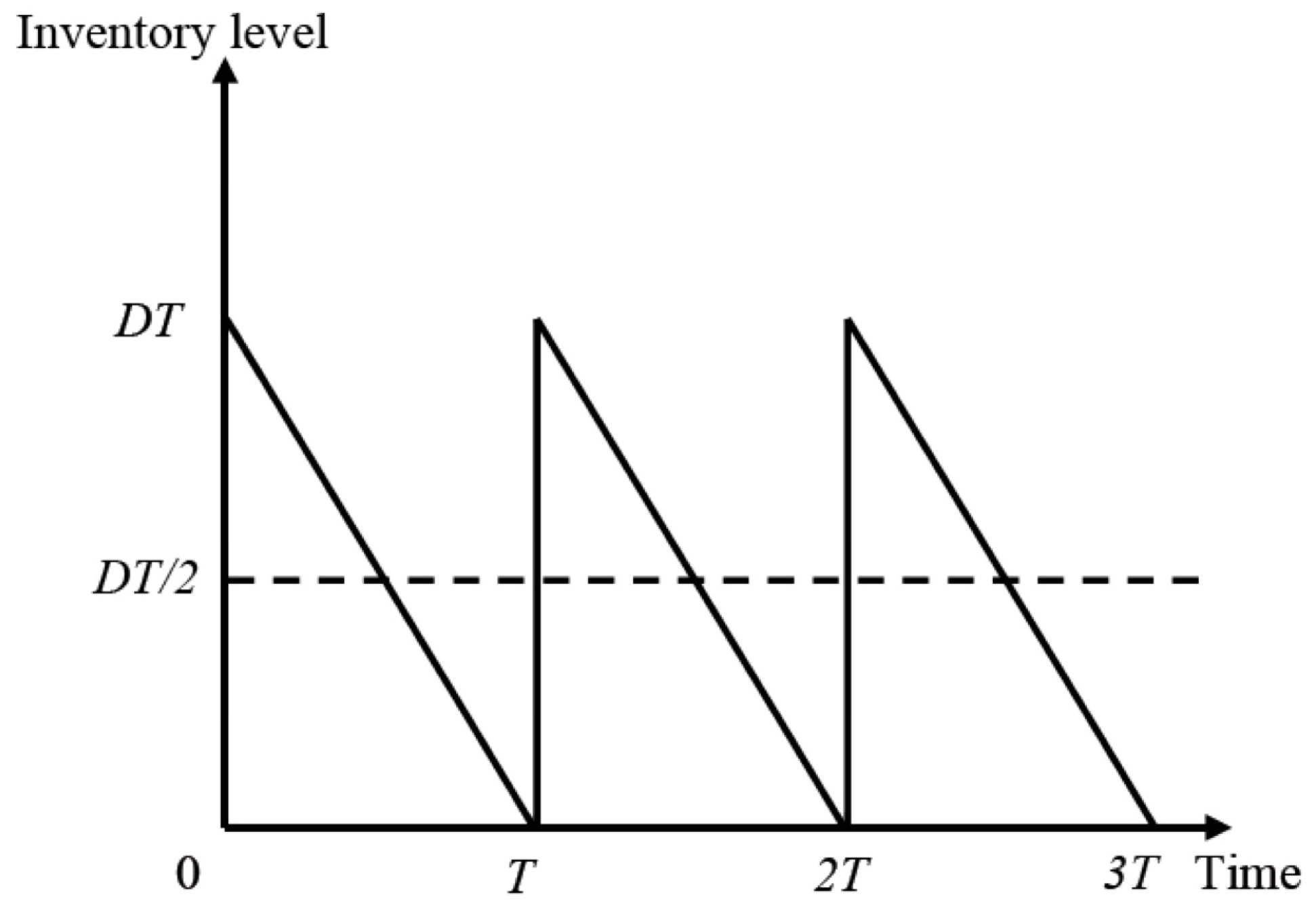
The annual holding cost (excluding interest charges) equals to
times the annual average inventory level
, as
Figure 1 shows. Therefore, the annual holding cost (excluding interest charges) is
.
- 3
The annual purchasing cost is .
- 4
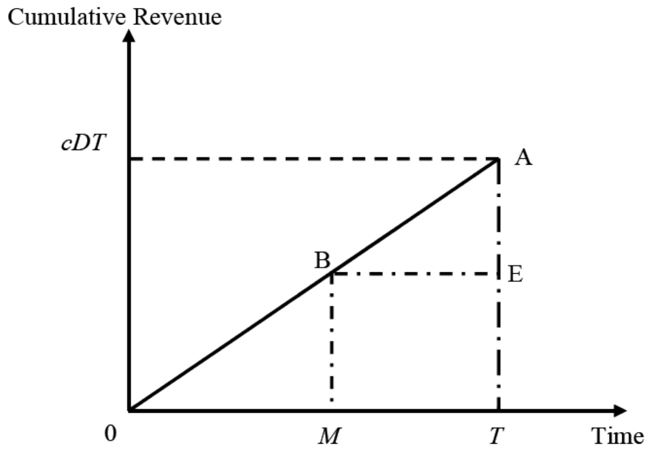
With regard to the costs of interest charges for unsold items after the credit period, according to Assumption 6, there are two cases to be considered.
Case 1:
. As the
Figure 2 shows, when
, the retailer pays off all units sold at time
, keeps the profits, and starts paying for the interest charges on the items sold after
. As a result, the interest payable per cycle is
times the area of the triangle ABE shown in
Figure 2. Therefore, the annual interest payable is
.
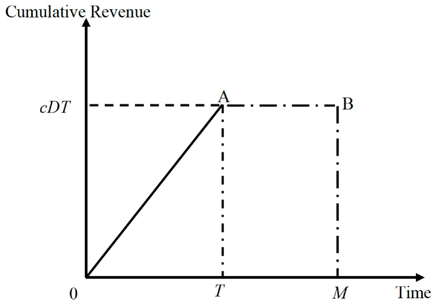
Case 2:
. In this case, the retailer can pay off the supplier at time
by all the sales revenue just as the
Figure 3 shows. Therefore, the annual interest payable is 0.
5 With regard to the interest earned from sales revenue, there are also two cases to be considered.
Case 1:
. As shown in
Figure 2, because the retailer only needs to pay off the purchase cost at time
, he/she can accumulate the revenue and earns the interest at a rate of
starting from time 0 through
. Therefore, the interest earned per cycle is
times the area of triangle OBM shown in
Figure 2. The annual interest earned is
.
Case 2:
. As
Figure 3 shows, the retailer starts selling the product at time 0 and receives the total revenue at time
. Moreover, he/she pays off all the purchase cost by
. Consequently, he/she earns the interest at rate
starting from time 0 through
. In this case, the interest earned per cycle is
times the area of trapezoid OABM shown in
Figure 3. The annual interest earned is
.
6 The emission cost (or revenue if ) is .
From the above arguments, the annual total cost for retailer is the total relevant cost (i.e., the sum of Assumptions 1–4 and 6) minus the interest earned. As a result, the annual total cost for the retailer is given by
where
Rearrange the terms of Equation (2) and substitute
into Equations (4) and (5), we obtain
Because
,
is continuous and well defined. Both
and
are defined on
. By taking the first and second derivatives of
and
, we obtain
Equations (9) and (11) imply that
and
are convex on
. In addition, we have
. Thus,
is convex on
. Let
for
, we get
According to the convexity of
and
, we can get
For furthering summarizing the results, we define , which determines the sign of the derivative of (i.e., and ) at (see Equations (8) and (10)). Moreover, we find that can be used to determine if the retailer’s optimal ordering cycle is larger or smaller than . This result is formally presented in Theorem 1.
Theorem 1. Under both the cap-and-trade system and trade credit financing, given the retailer’s annual total cost (Equation (3)), the retailer’s optimal ordering cycle is given by: (1) if , then and ; and (2) if , then and .
Proof. (1) If , then . Equation (14) implies that is decreasing on and increasing on , is decreasing on . Thus, is decreasing on and increasing on . As a result, .
(2) If , then . Equation (14) implies that is decreasing on and increasing on , is increasing on . Thus, is decreasing on and increasing on . As a result, .
Theorem 1 implies that
is an important term to determine if the optimal ordering cycle
is larger than credit period
. Note, if there is no cap-and-trade system, or equivalently the carbon price
equals to 0,
is degenerated to
, which has been discussed in Huang [
9] and Chung [
22]. Hence, their results are special cases of this research [
9,
22].
4. The Impacts of Carbon Emission Trading on the Retailer’s Ordering Policy
We investigate the joint impacts of trade credit and carbon emissions trading on the retailer’s ordering policy, carbon emissions and total cost in this section.
First, by investigating the expressions of , we find how the retailer’s optimal ordering cycle varies with the cost and carbon emissions, which is as the following Theorem shows.
Theorem 2. The is increasing in both A and e, and it is decreasing in both h and g.
Theorem 2 implies that the carbon emissions can be viewed as the extra costs that incurred during the ordering and inventory holding stages. That is, under the cap-and-trade system, the costs of the retailer that incurred during the ordering and stocking stages increase by pe and pg, respectively. On the one hand, if the retailer incurs more cost or emits more carbon dioxide per order, he/she inclines to order less frequently and extend the ordering cycle accordingly. On the other hand, if the retailer incurs more cost or emits more carbon dioxide during the inventory hold stage, the best strategy for him/her is to order less per time and shorten the ordering cycle. Under the cap-and-trade system, the retailer adjusts his/her ordering decisions accordingly on his/her carbon emissions during the ordering and inventory holding stages.
We next compare the costs minimizing ordering cycle with the cycle that minimizes the total emissions. This result is as Theorem 3 shows.
Theorem 3. - (1)
When :
- (a)
if , then ;
- (b)
if , then ; and
- (c)
if , then .
- (2)
When :
- (a)
if , then ;
- (b)
if , then ; and
- (c)
if , then .
Proof. Comparing with for the cases of and , respectively, it is easy to prove Theorem 3.
Theorem 3 makes a comparison between the optimal ordering cycle for the retailer under the cap-and-trade system, and the optimal ordering cycle that minimizes the retailer’s carbon emissions. Note that is the ratio of carbon emissions that emitted during the inventory holding stage to those emitted during the ordering stage. and are the ratios of the inventory holding cost to ordering cost when the retailer’s ordering cycle is shorter or longer than the credit period respectively. Theorem 3 implies that whether the retailer should order more products only depends on which of these two ratios is larger.
When (or ), the retailer’s optimal ordering cycle also minimizes the carbon emissions. That is, in this case, there is no space to further reduce the retailer’s carbon emissions by adjusting the retailer’s ordering and inventory decisions. However, when or , it implies that the carbon emissions during the inventory holding stages are relatively small. Thus, the retailer should order less and shorten his/her ordering cycles, compared with the ordering cycle that minimizes the total emissions. Therefore, is smaller than in this case, and vice versa.
Theorem 4. The retailer’s optimal ordering cycle is irrelevant to carbon cap . Moreover, given the carbon cap , we have the following.
- (1)
When :
- (a)
if , the retailer’s optimal ordering cycle is irrelevant to ;
- (b)
if , the retailer’s optimal ordering cycle is increasing in ; and
- (c)
if , the retailer’s optimal ordering cycle is decreasing in .
- (2)
When :
- (a)
if , the retailer’s optimal ordering cycle is irrelevant to
;
- (b)
if , the retailer’s optimal ordering cycle is increasing in ; and
- (c)
if , the retailer’s optimal ordering cycle is decreasing in .
Proof. By investigating the expression of (see Theorem 1), it is easy to observe that is irrelevant to . Moreover, differentiating with respect to , and letting the derivative be equal to, larger or smaller than zero, respectively, we can obtain the above conditions easily.
Theorem 4 further characterizes the varying of the retailer’s optimal ordering cycle under trade credit with the cap-and-trade system parameters. It implies that only the carbon price has impact on the retailer’s ordering decisions. More specifically, when (or ), the retailer’s optimal ordering cycle is increasing in carbon price, and vice versa. Note that is smaller than when (or ), it implies the retailer will always adjust his/her ordering cycle towards , which minimize the retailer’s total carbon emissions, as the carbon price increases.
To further investigate the impact of cap-and-trade system on the retailer’s cost and carbon emissions, we next consider the case where the price equals to zero. In this case, the retailer’s optimal ordering decisions degenerate to the case that there are no cap-and-trade system. In particular, we get , , and while applying equals to 0 to the expressions of , and respectively. Note the retailer’s optimal decisions, costs and emissions are all functions of carbon price, we denote this no cap-and-trade system case with , , , accordingly.
Corollary 1: The cap-and-trade system can induce the retailer to reduce carbon emissions, i.e., .
Proof. Omitted.
Corollary 1 implies that the cap-and-trade system can reduce the retailer’s carbon emissions as it is anticipated. However, what interests us now is how does the retailer’s cost change under this system, which is given in Theorem 5.
Let , , we have Theorem 5.
Theorem 5. - (1)
When and :
- (a)
if , the total cost ;
- (b)
if :
- (b.1)
if , then ;
- (b.2)
if , then ;
- (b.3)
if , then ; and
- (c)
if , then ;
- (2)
When and :
Let
- (a)
if , ;
- (b)
if :
- (b.1)
if , then ;
- (b.2)
if , then ;
- (b.3)
if , then ; and
- (c)
If , then ;
- (3)
When and :
- (a)
if , ;
- (b)
if ,
- (b.1)
if , then ;
- (b.2)
if , then ;
- (b.3)
if , then ; and
- (c)
if , then ;
- (4)
When and :
- (a)
if , the total cost
- (b)
if ,
- (b.1)
if , then ;
- (b.2)
if , then ;
- (b.3)
if , then ; and
- (c)
If , then .
Parts (1)–(4) of Theorem 5 are characterized with similar features. The retailer’s cost changes in the presence of cap-and-trade system can be divided into three cases by carbon cap. Firstly, if the carbon cap is less than the retailer’s minimum carbon emissions (i.e., ), the carbon constraint is so tight that the retailer has to buy carbon credit from the market anyway. As a result, the retailer’s cost will increase under common conditions, i.e., . However, this is not the case under some extreme conditions, such as when the cap-and-trade system alters the ordering cycle from longer than the credit period to shorter than the credit period (see Part (3) of Theorem 5). In this case, the cost changes are composed of two parts: on the one hand, the cost will increase because the extra carbon credit buying is needed; and, on the other hand, the cost will also decrease as the interest payable is reduced due to the shortened ordering cycle. As a result, if the cost changes are positive is dependent on the trade-off between these two effects.
Secondly, when the carbon cap is larger than (or ), Theorem 4 implies that the retailer’s cost will decrease generally except when the retailer’s optimal ordering cycle alters from shorter than credit period to longer than it under cap-and-trade system. Under this condition, because the increased interest payable may overstep the decreased emission cost, the retailer’s cost could increase Part (2) of Theorem 4 shows.
Finally, when the carbon cap is between the above two thresholds, Theorem 4 implies that the retailer’s total cost changes are dependent on the carbon price. If the carbon price is low, the cost will generally increase except the case that the retailer’s optimal ordering cycle alters from longer than credit period to shorter than it, and vice versa. As a result, a high carbon price is highly beneficial for reducing emissions and cost simultaneously.
Overall, compared to the modified EOQ model under cap-and-trade system that Hua et al. [
21] studied, our results show if the trade credit is considered, there is a joint impact of cap-and-trade system and trade credit on the retailer’s cost. On the one hand, the retailer incurs emission cost under the cap-and-trade system. On the other hand, the trade credit may also impact on the cost significantly when the retailer’s optimal ordering cycle changes from shorter/longer than the credit period to longer/shorter than credit period. The total cost changes are dependent on which of these two effects is larger.
Theorem 6. There exists thresholds and .
- (1)
When :
- (a)
if , then the retailer should buy units of carbon credit;
- (b)
if , then the retailer should sell units of carbon credit; and
- (c)
if , then the retailer should neither buy nor sell carbon credit.
- (2)
When :
- (a)
if , then the retailer should buy units of carbon credit;
- (b)
if , then the retailer should sell units of carbon credit; and
- (c)
if , then the retailer should neither buy nor sell carbon credit.
In Theorem 6, , and , respectively.
Proof. Let , , and , respectively, we can derive Theorem 6 easily.
Theorem 6 gives the threshold if the retailer should buy carbon credit from the carbon market. Under the trade credit mechanism, given the carbon cap, whether the retailer should buy carbon credit is not only determined by the ordering and holding cost of the inventory, but also determined by the credit period, the interest earned and the interest charged by the supplier. If the given cap is lower than the threshold or , the retailer should buy the carbon credit, and vice versa. The key insight here is that the retailer’s total emissions are irrelevant to the amount of carbon credits, i.e., the carbon cap allocated to the retailer, under the cap-and-trade system. The retailer would buy the carbon credit from the market once his/her emissions exceed the cap; otherwise, he/she would sell the extra carbon credit to earn revenue. As a result, though carbon cap does not influence the retailer’s total emissions, it determines how many carbon credits the retailer should buy or sell. In other words, it makes an impact on the retailer’s total cost.
Formally, we have the following theorem about the relationships between the carbon emissions and both the carbon cap and price.
Theorem 7. The carbon emissions are irrelevant to cap α' and decreasing in carbon price p.
This result is consistent with the fact. Moreover, the retailer’s carbon emissions are decreasing in carbon price as expected. Because the rising carbon price will not only increase the real cost, but also the opportunity cost of carbon emissions. The retailer has to adjust his/her ordering decisions and reduce the carbon emissions accordingly. However, we should note that marginal effect of carbon price on reducing the carbon emissions is decreasing as the carbon price rises. That is, when the carbon price is very high, the retailer’s optimal decision is similar to the one that minimizes emissions. No matter how high the carbon price is in this case, the lower bound of the emissions would never be exceeded.
Moreover, it should also be noted that the results in Theorems 6 and 7 are based on the assumption that the carbon cap are allocated to a single retailer. In fact, the carbon price will increase if the total carbon credits the government allocated to the system are reduced. The retailer’s ordering decisions and carbon emissions will be influenced by the increasing carbon price. As a result, the government could reduce the total carbon emissions by decreasing the total carbon credits allocated to the system.
Theorem 8. - (1)
When :
- (a)
if , the carbon emissions are increasing in , or else it is decreasing in ; and
- (b)
the carbon emissions are irrelevant to and .
- (2)
When :
- (a)
if , the carbon emissions are increasing in , and decreasing in and ; and
- (b)
if , the carbon emissions are decreasing in , and increasing in and .
Proof. By investigating the expression of carbon emissions , it is easily to prove Theorem 8.
Theorem 8 is composed of two cases. When the retailer’s optimal ordering cycle is shorter than credit period, the retailer’s carbon emissions are irrelevant to credit period and the difference between the interests charged and earned . Moreover, if , the retailer’s carbon emissions are increasing in . , and vice versa. When the retailer’s ordering cycle is longer than credit period and , the retailer’s carbon emissions are increasing in , and .
Similar to Theorems 3 and 4, the relationships between retailer’s carbon emissions and trade credit parameters , and also depend on the relative size of the ratios and (or ). Generally, if the retailer emits less at the inventory holding stage relative to the ordering stage, he/she would extend the ordering cycle to decrease the carbon emissions. However, if the interest earned is large, the retailer also inclines to shorten the ordering cycle because he/she would earn more interest. As a result, the retailer’s carbon emissions are increasing in . The similar reasons also apply to explain the relationships between carbon emissions and credit period and .
5. Conclusions
As global warming has become an increasingly important sustainability issue in today’s world, we study how the retailer to adjust his/her ordering decisions to reduce carbon emissions under the cap-and-trade system. In addition, because trade credit is a commonly used mechanism between suppliers and retailers, we incorporate it into our study to investigate how the retailer’s ordering policy changes under this condition. We derive the retailer’s optimal ordering cycle, as well as the total cost and carbon emissions, and compare them to those without cap-and-trade system. The main insights are summarized as follows.
First, the cap-and-trade system and trade credit financing jointly impact on the retailer’s ordering decision. The retailer’s optimal ordering cycle is increasing in ordering cost and emissions during the ordering stage. Moreover, it decreases with the cost and emissions during the storage stage. As a result, under the cap-and-trade system, the retailer would like to shorten his/her ordering cycle and order less products per time when he/she emits more carbon dioxide during the inventory holding stage relative to the ordering stage, such as for the deteriorating products (which need for refrigeration and emit more carbon dioxide during the inventory stage). On the other hand, considering one intention of the trade credit is to stimulate the retailer to order more each time, the effect of trade credit on stimulating the retailer to order more would be reduced in this case.
Second, our results imply the cap-and-trade system is effective in reducing the retailer’s carbon emissions. Moreover, under the cap-and-trade system, the retailer’s total cost may increase or decrease, depends on the carbon cap allocated to the retailer and the carbon price. Specifically, when the carbon constraint is too tight, the retailer has to buy carbon credit from the market anyway. Therefore, the retailer’s cost will increase except for some extreme cases. On the contrary, when the carbon cap or carbon price is very high, the retailer can reduce the cost and emissions simultaneously. Compared to the modified EOQ model under cap-and-trade system, which Hua et al. [
21] studied, we identify a few special cases that the cost changes oppositely to what Hua’s model predicts (such as Theorems 5(2) and 5(3) show), as a result of the joint impact of cap-and-trade system and trade credit on the retailer’s cost.
Finally, we find that the carbon cap does not impact on the retailer’s optimal ordering decisions and carbon emissions, but the total cost, as Theorems 4 and 7 show. Moreover, whether the carbon emissions are increasing in the trade credit parameters, such as annual interest earned per dollar, the difference between interest rate charged and earned, and the credit period is dependent on the relative size of the ratio and (or ). Throughout the paper, these ratios are key factors that determine the properties of retailer’s ordering cycle and carbon emissions. In addition, it is observed that trade credit only impacts on the cost ratio. At last, the retailer’s carbon emissions decrease with the carbon price, however, the marginal effect of carbon price on reducing carbon emissions is decreasing.
Based on EOQ model and taking trade credit into account, we investigate how the retailer adjusts his/her ordering decisions under the cap-and-trade system, and the corresponding changes of his/her carbon emissions and total cost. Our research could be extended from many perspectives. First, we could consider more complicate and realistic trade credit forms, such as the two-part or two-level trade credit, and investigate how the supplier and retailer coordinate under these conditions to reduce carbon emissions. The impact of carbon emissions constraint on the design of trade credit contract should be explicitly explored. Moreover, besides the cap-and-trade system, we could also examine the adjustment of the retailer’s ordering decisions under many other carbon control mechanisms, such as the strict carbon caps and the carbon tax, etc.
