Effects of New Roads on Environmental Resource Use in the Central Himalaya

Abstract

Construction of roads into remote rural areas can improve livelihoods by reducing transportation costs, but may also have negative environmental impacts, such as increased deforestation. However, evidence of the effect of rural roads on household environmental income and reliance, as well as local level forest stand conservation is limited. This study, conducted in Mustang District in Nepal, contributes to answering the following questions: (i) what are the impacts of the establishment of rural roads on household environmental income and reliance; (ii) what are the determinants of environmental income and reliance, and how are they affected by road establishment; and (iii) what are the short-term impacts of the construction of a rural road on local forest conservation? Following the Poverty Environment Network (PEN) methodology, income data from 176 randomly-sampled households were collected in 2006 from two similar Himalayan villages, Lete and Lulang, and again in 2012 after a new road was constructed in 2008 in Lete. Forest strata data were collected in Lete through permanent sample plots (n = 59) measured in 2005 and 2010 and used to estimate stock change (before and after road construction), annual increment and annual wood extraction. Results show that the new road had significant positive effects on absolute household environmental income, but negative effects on reliance as other income options became available. Wood product extraction levels remained below increment levels, indicating that the road did not (yet) have negative implications for local forest conservation.

1. Introduction

Rural household incomes in developing countries derive from diverse activities [1,2,3,4], typically in response to variations in household member skills, the seasonality of employment opportunities and food production systems, shocks and spatially in relation to market access [1,3]. Recently, the economic importance of income (absolute and relative) from forests and other non-cultivated environments—such as grasslands, fallows, rivers and swamps—to rural households has been demonstrated across a range of developing countries and settings (e.g., [4,5,6,7,8]). Both rich and poor rural households benefit from such environmental income, with the average contribution to total household income varying across regions: 32.1% in Latin America, 22.0% in Asia and 30.1% in Africa [4]. With some exceptions [7,9], most studies find higher environmental reliance (i.e., relative share of environmental income in total household income) among poorer households and that richer households tend to have higher levels of absolute environmental income [4,8,10,11]. Generally, environmental income is integrated into rural livelihoods through: (i) supporting current consumption (e.g., [12,13]); (ii) gap filling in periods with a lack of other income (e.g., [14]); and (iii) the provision of safety-nets in response to common and idiosyncratic shocks depressing income and food security (e.g., [14]). Furthermore, there may be situations where environmental income contributes to providing pathways out of poverty [3,15,16].

Given the importance of environmental income to rural livelihoods, such income should be explicitly considered in poverty alleviation interventions and policies [4]. To identify appropriate interventions and policies, a better understanding of the nature and dynamics of environmental income is needed. Published studies are mostly static, and the available panel datasets usually do not account for environmental income. However, environmental income and reliance change in response to a range of factors, such as relative prices and employment opportunities. Such factors are substantially influenced by road infrastructure, and hence, the establishment of new roads into remote rural areas, reducing the costs of transporting agricultural and other products to markets [17]. Transport costs are often the single most important cost of agricultural production and marketing in rural areas [18].

Despite the accepted fact that road establishment in rural areas in developing countries can bring about economic and social benefits to the affected villages [19,20,21], it can also have negative environmental consequences, e.g., through immigration-driven land conversion or increased harvesting of environmental resources to supply urban markets. This can lead to deforestation, landscape fragmentation, increased landslides, the spread of invasive species and the depletion of wildlife by commercializing former local subsistence hunting [22,23,24,25,26,27,28,29,30,31]. New roads opening access to remote areas are considered a major factor contributing to deforestation in Nepal [32]. Extraction of fuelwood, construction material, fodder and other forest products can also reduce stocks and biodiversity. Trade-offs may therefore exist between conservation and development objectives in relation to road development, and assessment of the impacts of roads on forest product extraction and stocks is needed to facilitate informed decisions in the designing of conservation strategies.

The impact of roads on poverty in developing countries has been subject to recent scrutiny [33,34,35]. However, most studies addressing the household-level impact of roads focus on broad outcome measures, such as total household income, with no disaggregation to specific income sources. Very few studies have assessed the impacts of road establishment on non-farm income [36,37]. Additionally, no studies have assessed the impact of road establishment on household environmental income and reliance, hindering an understanding of the overall impacts and making the abovementioned trade-offs difficult to evaluate.

This study provides an empirical investigation of the counterfactual effect of road establishment on household-level environmental income and associated determinants, linked to changes in forest stock in the Central Himalayas through a BACI analysis (Before, After, Control and Implementation). The research questions are: (i) what are the impacts of the establishment of rural roads on household environmental income and reliance; (ii) what are the determinants of environmental income and reliance, and how are they affected by road establishment; and (iii) what are the short-term impacts of rural road construction on local forest conservation? This is achieved through a quasi-natural experiment using a panel dataset providing household-level total income data from one site—Lete Village Development Committee (VDC, an administrative unit) in Mustang District—before and after rural road construction, and a control site—Lulang VDC in Myagdi District without road establishment. Both sites are located in the high mountain physiographic zone of the Western Development Region of Nepal. Income data cover the years 2006 and 2012, while the road providing access to urban centers was constructed through Lete VDC in 2007/2008 and opened in 2008.

2. Methods

2.1. Study Sites

Lete and Lulang VDCs (Figure 1) are located above 2000 m.a.s.l. and experience similar weather patterns, with most of their precipitation received in the four months from June to September coinciding with the peak farming season. The terrain is highly variable, with grasslands on rugged steep mountain slopes, forest in the mid-slopes and plateaus and cultivated river valleys. Livelihoods generally rely on agriculture, livestock production, forests products and small-scale trade/business. All crop production relies on rain-fed irrigation. Herds of sheep and goats move from grazing in agricultural plots, for fertilization before planting, to forests and high altitude grassland after planting. Cattle and buffalo are normally kept in the villages and supplied cut-and-carry fodder from forest and non-forest environments. Trekking routes through Lete and Lulang provide tourism income, although trekking is more popular in Lete than in Lulang. In both sites, remittances constitute an important source of income.

The areas have relatively low population density and high forest area per capita (compared to lower altitudes). The forest is dominated by Pinus wallichiana A.B. Jacks and some old-growth Tsuga dumosa (D. Don) Eichler, two valuable timber species. In both study sites, forest products, such as fodder and firewood, are usually harvested by individual households. Forests are government owned, but communities have use and management rights, and there is a high degree of rule enforcement. Lete VDC is located inside the Annapurna Conservation Area, and forest management has since 1992 been implemented through Conservation Area Management Committees (CAMCs) monitored by the National Trust for Nature Conservation, a national conservation-oriented non-governmental organization. In Lulang VDC, local forest user groups are required to submit management plans detailing rules for the collection of firewood and non-timber forest products, the annual allowable cut of timber, rotational harvesting and regeneration, among others, to the Department of Forests (DoF) for approval. The DoF usually limits firewood collection to dead wood and sets a low quota for timber extraction for community or personal purposes.

Lete VDC, in Mustang, is today approximately a four-hour bus ride from Myagdi District headquarters, Beni, along the newly-constructed Beni-Jomsom-Sadak road, which continues to the headquarters of Mustang District (Jomsom; about three hours from Lete). This dry weather tertiary road provides vehicular access to markets, hospitals, schools and other major facilities. Lulang VDC, in Myagdi, remains remote with no road connection to neighboring town centers. The nearest dry weather road is located in Darbang, about eight hours' walking distance from Lulang. The construction of a dry weather road from Darbang to Takum (four-hour walk from Lulang) began in 2012, but was not completed at the end of this study.

2.2. Data Collection

The Lete (n = 74) income data are a panel dataset, designed and collected following the Poverty Environment Network (PEN) approach [38], where households were randomly selected through a computer-generated random table, produced from an up-dated census list sourced from the VDC office. Data collection included rural appraisal at VDC and village levels to generate contextual understanding used to adapt the prototype questionnaire to the local context; translation of the prototype questionnaire into Nepali; and testing outside the frame. Income data were collected using four quarterly surveys in 2006 and repeated in 2012. In Lulang (n = 102), the same format was applied to collect data for both years, based on recall, in the beginning of 2013. To minimize the bias of a longer recall period, we implemented a methodology similar to Krishna’s stages-of-progress approach [39,40]. Respondents were reminded of major event(s) in 2006, e.g., the end of the civil war, and the 2006 questionnaire was implemented after a conversation about life in that period to help jog memory.

All 2012 prices were converted to 2006 prices using the national Consumer Price Index (CPI). Income is defined as the gross value obtained from the trade/consumption of goods and/or services by members of the household, minus the cost of all inputs and capital, except for the cost of household labor. It thus includes both cash and subsistence income. The survey recorded income from seven major sources: environmental, crop, livestock, business, wage, remittances and other income. Valuation techniques followed Wunder et al. [41]. Environmental income is the sum of benefits resulting from the extraction of forest and other non-cultivated wild products (from grasslands, swamps, fallows, etc.). Also included is income from Forest User Group (FUG) payments and processed environmental products. Crop income is generated from the production of agricultural crops. Livestock income includes income from farm animals and any products and services they provide. Wage income includes income from wage work, whether on or off farm. Business income refers to income from private business, other than farms, owned and managed by the household. Income received from family members living and working away is referred to as Remittance income. Other income is income not accounted for above (e.g., from pensions). Total annual household income is the sum of all sources of household income throughout a 12-month period. The relative share of each income source in total household income was calculated, reflecting household reliance. All income measures are converted to adjusted Adult Equivalent Units (AEU) [5].

Lete’s forest area (501 ha between approximately 2000 and 2900 m) was stratified into seven strata, based on forest structure and species-level basal area. The seven forest strata (S) are shown in Figure 2 (S.1–S.7). S.1 consists of young to middle-aged stands of P. wallichiana, some of which are planted. The stands are located in flat terrain east of Lete, along the banks of the Kali Gandaki River, and in sloping terrain west of Lete. S.2 is heavily degraded forest in sloping terrain west of Lete, where almost no larger trees are left. S.3 is mixed forest dominated by T. dumosa and P. wallichiana. It is degraded from past timber extraction and fire. S.4 is located on north-facing slopes south of Lete; it is a dense forest with typical characteristics of virgin forest with many large old trees and large amounts of deadwood. S.5 is upper-slope forest west of Lete and is dominated by T. dumosa and Rhododendron arboreum Sm. S.6 is mature, mixed forest with P. wallichiana and broadleaves, such as Juglans, Ilex and Rhododendron. S.7 is mixed P. wallichiana forest, partly with a middle story of Alnus nepalensis D. Don, and is located along the Kali Gandaki River.

A total of 59 permanent plots (500 m² each) were established in 2005, using a nested plot design. The spatial distribution of the plots followed a “coffee-house” design within each of the seven forest strata [42]. In our implementation of the coffee-house design, the first point/plot is located randomly within the relevant area (polygon), and all subsequent points are located in the position that is optimal given the location of all previously-established points (see Appendix 1 for further explanation of the coffee-house design). Their actual geographical location was recorded using a GPS device, and corners were marked using concrete pillars. Measurements within plots included tree species identification, stem mapping and diameter at breast height for all trees. Total tree height, bole height, tree health and quality were measured for a permanent sample of trees selected for each species (289 trees in 2005, 263 trees in 2010). Trees that reached a sufficient diameter between 2005 and 2010 were recorded as ingrowth. Trees felled between 2005 and 2010 (stumps) were recorded as harvested.

2.3. Data Analysis

Using household economic data, we document the economic importance of environmental income to rural households, followed by an estimation of the impact of the road on absolute and relative environmental incomes. We then examine the household-level characteristics affecting these incomes, through parameterized structural models. Random effects models were estimated for environmental income and environmental reliance to determine the effects of the road and other household-level covariates over the observation period. Random effects models were chosen over fixed effects models based on the Hausman test (probability > χ² = 0.4056). The models were estimated with errors clustered by villages for increased robustness. The covariates used in model specification were selected based on empirical relations observed in the literature (

Table 1. Overview of expected relationships between covariates and Environmental Income (EI) and Environmental Reliance (ER) at the study sites. AEU refers to Adult Equivalent Units; FUG to Forest User Group.

Variables	Expected Signs		Guiding Assumptions
	EI	ER
Road
1. Interaction term showing the effects of the road on the affected village (Village×Time)	+	−	The road will increase access to markets where environmental products fetch higher prices, thus increasing environmental income; however, due to greater access to town centers, households will be less reliant on this income source in Lete.
Location in region
2. Village dummy (treatment: Lete = 1; and control: Lulang = 0)	−	−	Environmental income and reliance is lower in the treatment village (Lete) because more remunerative income-generating options are present, especially after the construction of the road.
Time
3. Time dummy (after: 2012 = 1 and before: 2006 = 0)	−	−	As households accumulate assets, they invest in more remunerative income sources; therefore, both environmental income and reliance decline.
Household characteristics
4. Age of household head	−	−	Younger households tend to have higher absolute and relative environmental income because of a lack of assets [7,11]. However, the opposite can also be true in some cases, as older households are not able to practice farming and may rely more on environmental income.
5. Gender of household head (female = 1)	−	+	Female-headed households have less labor available for the extraction of environmental resources; however, they also have fewer assets and may therefore depend more on environmental income [11,44,45].
6. Household head education	−	−	Number of years of formal schooling completed. Better-educated households have greater access to more remunerative income options [4,11,15].
7. Dependency ratio	+	+	Ratio of dependents (children <15 years and adults >60 years) to laborers. A high ratio means fewer household members are able to participate in other income-generating activities, making environmental income more important.
Household assets
8. Total value of implements Ω owned by household (AEU)	−	−	Higher values indicate access to other income-generating activities and less reliance on environmental income [6,46].
9. Area of crop land cultivated by household	+	−	Crop land is fertilized using compost, which contains forest products; therefore, environmental income will be higher, while reliance will be lower as households produce more crop income [44].
10. Area of land rented by household	+	+	Following from above, absolute environmental income is higher with more land is rented, but households renting land are poor and, therefore, more reliant on the environment [6,11,15].
11. Area of other land owned by household	+	+	Other land is uncultivated land, where environmental products can be extracted, increasing environmental income and reliance.
12. Household savings (AEU)	−	−	Savings can be invested in more remunerative income-generating activities, as well as provide a buffer against shocks, reducing environmental income and reliance [11].
13. Household debt (AEU)	+	−	Debt may signal access to credit used to invest in production options, making households less reliant on environmental income, though they may earn high absolute values [11].
Location in village
14. Distance to village center in minutes	+	+	Households on the village edge are closer to environmental harvest areas (forest, fallows and pastures), leading to higher absolute and relative values [7,47].
FUG influence
15. Household participation in FUG activities (yes = 1)	+	+	Households participating in FUG activities invest time into forest management and have more influence on the use of resources. Therefore, they are likely to earn higher environmental income and be more reliant on this income source.

^Ω These include all productive implements used in crop production, livestock production, collection of environmental products and the processing of all raw material.

). Hence, the model is a linear random effects panel data model where environmental income or environmental reliance is given by:

$$y_{it}^j=\mathsf{\alpha }+{\mathsf{\alpha }}_1{d}_t+{\mathsf{\alpha }}^1{d}^j+\mathsf{\beta }{d}_t^j+Z_{it}^j\delta +{Є}_{it}^j$$

(1)

where y is the outcome variable of interest for unit i (household: i = 1, …, N_t) in group j (control = 0 or treatment = 1) in period t (2006 = 0 or 2012 = 1), where road establishment acts as the treatment. d_t, $d^j$ and $d_t^j$ are dummy variables, where: d_t = 1 if t = 1 and 0 otherwise; $d^j$ = 1 if j = 1 and 0 otherwise; $d_t^j$ = 1 for the treated group after it receives the treatment and 0 for all other cases. β is the true causal effect of the treatment on the outcome for the treated group. The key identifying assumption is that β would be 0 in the absence of the treatment or $E[{Є}_{it}^j|d_t^j]=0$. Additionally, $Z_{it}^j$ represents the vector of household-level characteristics, allowing us to adjust for observable differences between the observations in the different groups. Enforcing equality of $\mathsf{\delta }$ across groups ensures that Equation (1) will adjust for differences in these variables across groups [43].

All variables and the theoretical justification for including them in the models are explained in Table 1. The first variable in the models is an interaction term between the location, i.e., the treatment-control dummy and the time dummy representing the situations before and after road construction reflecting the counterfactual effect of the Beni-Jomsom-Sadak road on environmental income or reliance in Lete. Then follows the individual location and time dummies, reflecting the treatment and control villages and the time period prior and subsequent to the road construction. The other covariates grouped under household characteristics provide proxies for labor force and skills available to a household, while the household asset covariates act as proxies of household wealth status. Given the weak land markets in the region, land is considered a proxy for more permanent wealth, along with productive implements, while savings and debt may tend to fluctuate more easily. Livestock value was highly correlated with the age of the household head and the value of implements and, therefore, was dropped from the model. The final two covariates account for the household’s distance from the village center (which is normally where transportation and market hubs are located) and the household’s participation in forest and environmental management activities at the village level.

Having determined the effects of the road and household-level determinants of environmental income and reliance, we examine how significant household-level determinants modify the effects of the road on the outcome variables. This is done through the inclusion of interactions between the road effects dummy and specific covariates in the model.

The volume of trees alive in 2005 and 2010, dead, but still present in 2010, harvested between 2005 and 2010 and ingrowth detected in 2010 and total wood volume (m³·ha⁻¹) were estimated using Sharma and Pukkala’s functions [48] for total volume in each of the 59 forest plots. Total volume includes volume <10 cm in diameter, which is an important source of firewood, and volume >10 cm in diameter, which is mainly used for construction purposes. Estimates of standing stock in 2005 and 2010 and the increment were calculated at the plot, stratum and forest level and compared to the estimated extraction. Stratum-level estimates were calculated using standard methods for unconstrained random samples, whereas forest-level estimates were calculated using methods for stratified random sampling.

3. Results

3.1. The Dynamics of Household-Level Environmental Income

Basic statistics for absolute and relative household-level incomes per year for each source are presented in

Table 2. Household (n = 176) income (USD per AEU) per income source in 2006 and 2012, Nepal, Central Himalayas (percentage shares in parentheses).

Income Source	Lete (n = 74)		Lulang (n = 102)		Total Sample (n = 176)
	2006	2012	2006	2012	2006	2012
Environmental income	166 ± 154 (18.3)	149 ± 178 (16.7)	210 ± 159 (42.5)	197 ± 179 (52.7)	191 ± 158 (28.7)	177 ± 180 (29.9)
Crop income	40 ± 57 (4.5)	24 ± 65 (2.7)	29 ± 22 (5.8)	20 ± 17 *** (5.4)	34 ± 41 (5.0)	22 ± 44 *** (3.7)
Livestock income	117 ± 209 (12.9)	54 ± 79 ** (6.0)	149 ± 152 (30.1)	96 ± 85 *** (25.7)	135 ± 178 (20.3)	78 ± 85 *** (13.3)
Remittances	20 ± 67 (2.2)	90 ± 266 ** (10.1)	62 ± 130 (12.5)	34 ± 89 (9.1)	44 ± 110 (6.6)	57 ± 187 (9.7)
Business income	463 ± 819 (51.1)	302 ± 557 (34.0)	5 ± 28 (1.1)	5 ± 17 (1.2)	198 ± 576 (29.6)	130 ± 389 (22.0)
Wage income	19 ± 34 (2.0)	25 ± 48 (2.8)	19 ± 37 (3.9)	17 ± 31 (4.4)	19 ± 36 (2.8)	20 ± 39 (3.4)
Other income	82 ± 121 (9.0)	246 ± 495 *** (27.7)	21 ± 64 (4.2)	6 ± 18 ** (1.5)	46 ± 96 (7.0)	107 ± 341 ** (18.1)
Total income	906 ± 850	888 ± 810	494 ± 306	374 ± 256	667 ± 630	590 ± 613

Standard deviation after ±. Significance levels of change from 2006 to 2012 (pair-wise t-test): *** p < 0.01; ** p < 0.05.

. The share of environmental income in total household income averaged 29% in 2006 and 30% in 2012 (average of both VDCs), derived mainly from fuelwood, timber, medicinal plants, wild fruits, wild vegetables, leaf litter, bamboos and grasses for fodder and roof construction. The standard deviation is large for all seven income categories (and total income), and the comparison of mean and median values indicates a considerable skew between households in the study villages (see Appendix 2).

Overall, business income was the dominant source of household income in Lete in both periods (51% in 2006 and 34% in 2012), while environmental income contributed the highest share in Lulang (43% in 2006 and 53% in 2012). In Lete, the share of environmental income in overall household total income remained constant at 17%–18% in 2006 and 2012. Livestock income for both VDCs contributed an average of 20% in 2006 and 13% in 2012, while crop income only provided on average 5% in 2006 and 4% in 2012, reflecting small land holdings and low productivity in the high mountainous regions.

Average total household income in the period dropped by 77 USD (11.5%) mainly due to reduced business and livestock incomes. Absolute mean environmental income dropped across the period from 191 USD to 176 USD (7.9%). In Lete, absolute livestock income dropped significantly (p < 0.017), while remittances and other income increased significantly (p < 0.030 and p < 0.006) (pair-wise t-test). In Lulang, crop income, livestock income and other income all significantly decreased (p < 0.001, p < 0.002, p < 0.024, respectively).

Most environmental income is subsistence income (Figure 3a). In Lete, households on average doubled their cash environmental income after establishment of the road while overall subsistence environmental income declined sharply. However, while 99% of households obtained subsistence environmental income, only 54% were involved in the trade of environmental products for cash. Further disaggregating by wealth terciles in Lete reveals that most of the increase in cash environmental income was recorded among the two poorest terciles (Figure 3b). Additionally, the poorest households did not experience a drop in subsistence environmental income. There were no significant changes in levels of cash and subsistence environmental income in Lulang between the two years of observation.

3.2. The Impacts of Road Establishment

The outputs of the random effects models of environmental income and reliance are presented in

Table 3. Random effects models of EI and ER.

Covariates	Parameterized Structural Models
	EI		ER
	Coefficeint	Robust Standard Errors	Coefficient	Robust Standard Errors
Interaction term: road effects (β)	25.575 ***	1.685	−0.068 ***	0.018
Village dummy	−92.821 ***	14.231	−0.135 ***	0.007
Time	−12.004	6,654	0.074 ***	0.002
Age of household head	0.724	1.452	−0.0001	0.001
Gender of household head	38.897	26.624	0.030	0.020
Household head education	1.441	1.060	−0.004 ***	0.001
Dependency ratio	28.711 ***	3.711	0.040 **	0.017
Value of implements (AEU)	−0.150 ***	0.004	<−0.001 ***	0.000
Area of crop land (m2/AEU)	0.012 ***	0.001	<−0.001	0.000
Area of land rented in (m2/AEU)	0.054 ***	0.004	<0.001	0.000
Area of other land (m2/AEU)	0.019 ***	0.002	<0.001	0.000
Savings (AEU)	0.001	0.000	<−0.001	0.000
Debt (AEU)	−0.003	0.006	<0.001 ***	0.000
Distance to village center (min)	0.609 ***	0.180	<0.001	0.000
Participation in FUG activities	13.439	11.490	−0.053	0.069
Constant	98.554 **	48.63	0.465 ***	0.021
	N = 176		N = 176
	Rho = 0.484		Rho = 0.384
	Overall R-sq = 0.116		Overall R-sq = 0.343

Significance levels: *** p < 0.01; ** p < 0.05.

(see Appendix 3 for basic statistics for the covariates). Road establishment had a significant positive effect on household-level environmental income in Lete VDC. Results also show that a higher dependency ratio, area of land (crop land, land rented, other land) and distance to village center were significantly associated with higher environmental income, whereas a higher value of implements owned had a significant negative effect on environmental income.

Establishment of the road also appears to have a significant negative effect on household-level environmental reliance in Lete VDC, although households in the study area generally became more reliant on environmental income over time (cf. above). A higher household dependency ratio and level of debt both had a significant positive effect on environmental reliance, while higher levels of household head education and value of implements owned were significantly associated with lower environmental income.

To understand how the covariates of environmental income and reliance modified the road effects, we consecutively included interaction terms in the models (Appendix 4). In the model of absolute environmental income, the positive effects of road establishment on environmental income were significantly reduced by the value of implements and the area of other land owned by the household. The household’s dependency ratio, area of crop land owned and area of land rented in significantly increased the effects of the road on environmental income. In other words, the positive effects of road establishment were lower for households with a higher value of implements and households that owned larger areas of other land, while they were higher for households with more dependents, households with greater areas of crop land and land rented. In the model of environmental reliance, the value of household implements and the level of debt significantly reduced the negative effects of road establishment.

3.3. The Impacts of Road Establishment on Forest Conservation

Standing volume (V) in 2005 and 2010, annual increment and annual extraction were estimated for each of the seven forest strata and for the entire forest in Lete (

Table 4. Estimates of stock change (2005 to 2010), increment and extraction of wood (total) based on permanent sample plots (n = 59) in Lete, Mustang District, Nepal. Standard errors are shown in parenthesis.

Stratum No.	Area of Stratum (ha)	Standing Stock		Change of Stock (m3·ha−1)	Increment b (m3·ha−1)	Annual Values			Extraction Increment Ratio
		V2005 (m3·ha−1)	V2010 a (m3·ha−1)			Increment (m3·ha−1·Year−1)	Extraction (m3·ha−1·Year−1)	Increment Surplus (m3·ha−1·Year−1)
S.1	56.5	281.3	306.3	25.0	37.0	7.4	2.4	5.0	0.32
		(35.7)	(35.3)	(7.3)	(5.0)	(1.0)	(1.0)	(1.5)
S.2	16.1	7.5	11.3	3.8	3.8	0.8	0.0	0.8	0.00
		(4.1)	(4.1)	(1.9)	(1.9)	(0.4)	(0.0)	(0.4)
S.3	71.4	142.6	164.2	21.6	30.4	6.1	1.5	4.5	0.25
		(35.9)	(37.8)	(12.3)	(9.8)	(2.0)	(0.9)	(2.4)
S.4	170.3	401.6	408.2	6.5	12.5	2.5	1.1	1.4	0.42
		(110.6)	(113.5)	(6.4)	(5.4)	(1.1)	(0.3)	(1.3)
S.5	23.1	210.9	222.6	11.7	15.1	3.0	0.7	2.3	0.22
		(73.4)	(75.4)	(2.6)	(3.0)	(0.6)	(0.3)	(0.5)
S.6	115.1	207.7	225.8	18.1	18.5	3.7	0.1	3.6	0.02
		(67.0)	(74.5)	(9.5)	(9.5)	(1.9)	(0.1)	(1.9)
S.7	48.3	136.9	153.0	16.1	17.5	3.5	0.3	3.2	0.08
		(13.1)	(14.3)	(6.2)	(7.4)	(1.5)	(0.3)	(1.2)
Forest-level	500.8	259.6	274.1	14.5	19.5	3.9	0.9	3.0	0.24
estimates		(41.3)	(42.9)	(3.7)	(3.3)	(0.7)	(0.2)	(0.7)

^a Standing stock in 2010 is estimated as the sum of the volumes of live trees and ingrowth; ^b the increment is estimated as the difference in the volume of live trees in 2010 and 2005, plus the volume of ingrowth.

). In 2005, the standing stock estimated for the forest as a whole was 259.6 m³·ha⁻¹. At the stratum level, the standing stock varied considerably, with the lowest standing volume observed in S.2 (7.5 m³ ha⁻¹). This stratum is heavily degraded and affected by livestock browsing. Two other strata are also degraded, but to a lesser extent: S.7 (136.9 m³·ha⁻¹) southeast of Lete and S.3 (142.6 m³·ha⁻¹) immediately above Lete, where most P. wallichiana was harvested in the past and 61% of the remaining stock is T. dumosa. Higher volume levels were observed in S.1 (281.3 m³·ha⁻¹), which includes almost pure, even-aged and even-planted stands of P. wallichiana, S.5 (210.9 m³·ha⁻¹), where T. dumosa and R. arboreum are the most dominant species, and S.6 (207.7 m³·ha⁻¹), where the main species is P. wallichiana. The highest standing volume (401.6 m³·ha⁻¹) was observed in S.4 located on a relatively steep north-facing slope south of Lete and constituting an almost undisturbed, mixed forest dominated by T. dumosa and P. wallichiana.

Standing stock increased in all seven forest strata from 2005 to 2010. The forest-level change of standing stock was 14.5 m³·ha⁻¹, varying from 3.8 m³·ha⁻¹ in S.2 to 25 m³·ha⁻¹ in S.1. The forest-level mean annual stock increment was 3.9 m³·ha⁻¹·year⁻¹, varying from 0.8 m³·ha⁻¹·year⁻¹ in the degraded S.2 to 7.4 m³·ha⁻¹·year⁻¹ in the even-aged P. wallichiana stands in S.1. The forest-level mean annual extraction was 0.9 m³·ha⁻¹·year⁻¹, ranging from 0.0 m³·ha⁻¹·year⁻¹ in the degraded S.2 to 2.4 m³·ha⁻¹·year⁻¹ in the even-aged P. wallichiana stands in S.1. In all strata, the estimated mean annual extraction was lower than the mean annual increment. The mean increment surplus varied from 0.8–5.0 m³·ha⁻¹·year⁻¹. The standard errors of the estimated mean increment surplus values were lower than the estimated values, and the overall-forest level estimate is significantly different from zero (mean ± 95% CI: 3.0 ± 1.5 m³·ha⁻¹·year⁻¹, probability > |t| < 0.001). The proportion of the increment that was extracted in the five-year period varied from 0.00 in the degraded S.2 to 0.42 in the almost undisturbed S.4, and for the forest as a whole, it was only 0.24. It thus seems that harvest can be increased considerably in all strata, except the most understocked ones (S.2, S.3, S.7) without reducing standing stock. Considering only the increment surplus of the four strata with a stocking in 2010 of at least 200 m³·ha⁻¹, the annual extraction level could be increased by as much as 1000 m³·ha⁻¹·year⁻¹ without jeopardizing forest stocking. Since the present extraction is only 462 ± 214 m³·ha⁻¹·year⁻¹ (mean ± 95% CI), this corresponds to tripling the extraction.

4. Discussion

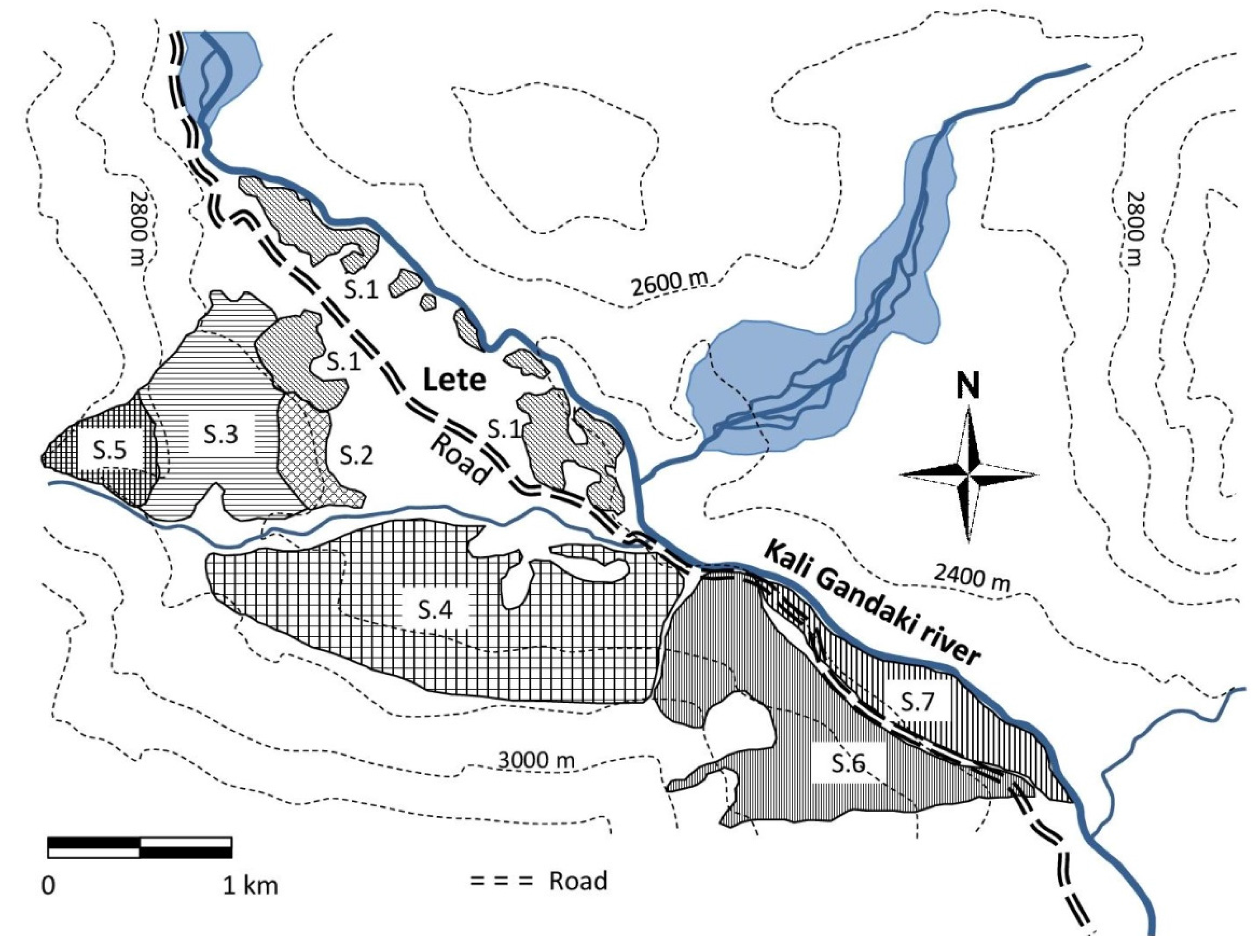
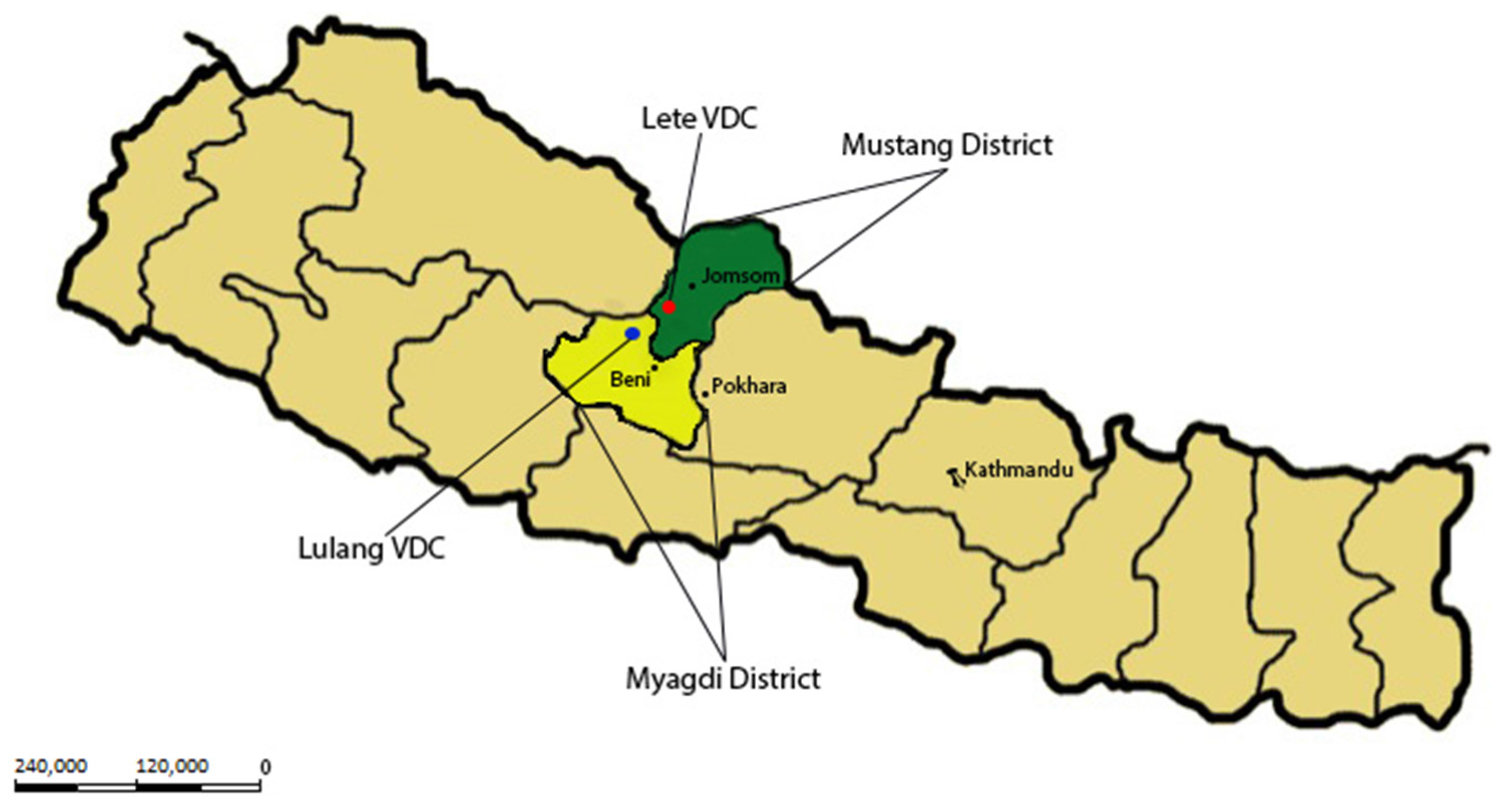
4.1. Rural Roads and Environmental Income in the Nepal Himalayas

Our findings confirm the importance of environmental income to rural households in the Western Himalayan region of Nepal, matching that of similar studies [11,49]. Environmental income mainly originated from the collection of environmental products consumed in households (subsistence). High-return forest activities, such as logging and timber cutting, are discouraged, as conservation is one of the primary objectives of forest management in the Annapurna Conservation Area.

Between 1999 and 2003, investment in road construction accounted for 5.7% (over USD 200 million) of Nepal’s national budget [50], as such interventions are expected to have strong positive effects on rural household welfare [50,51]. Using the same dataset as the one utilized in this study, another study by Charlery et al. [17] found that rural road construction had a significantly positive effect (to the magnitude of 28%) on household total income in the Western Himalayan region of Nepal. Our results show that after the construction of the road through Lete, a greater proportion of environmental products is now sold for cash. This is a direct result of the improved access to the town centers of Beni, Jomsom and beyond. Previously, most agricultural and environmental products were used for household subsistence, and any surplus was mainly traded among villagers. Similar trends have been noted in other studies, such as Shah et al. 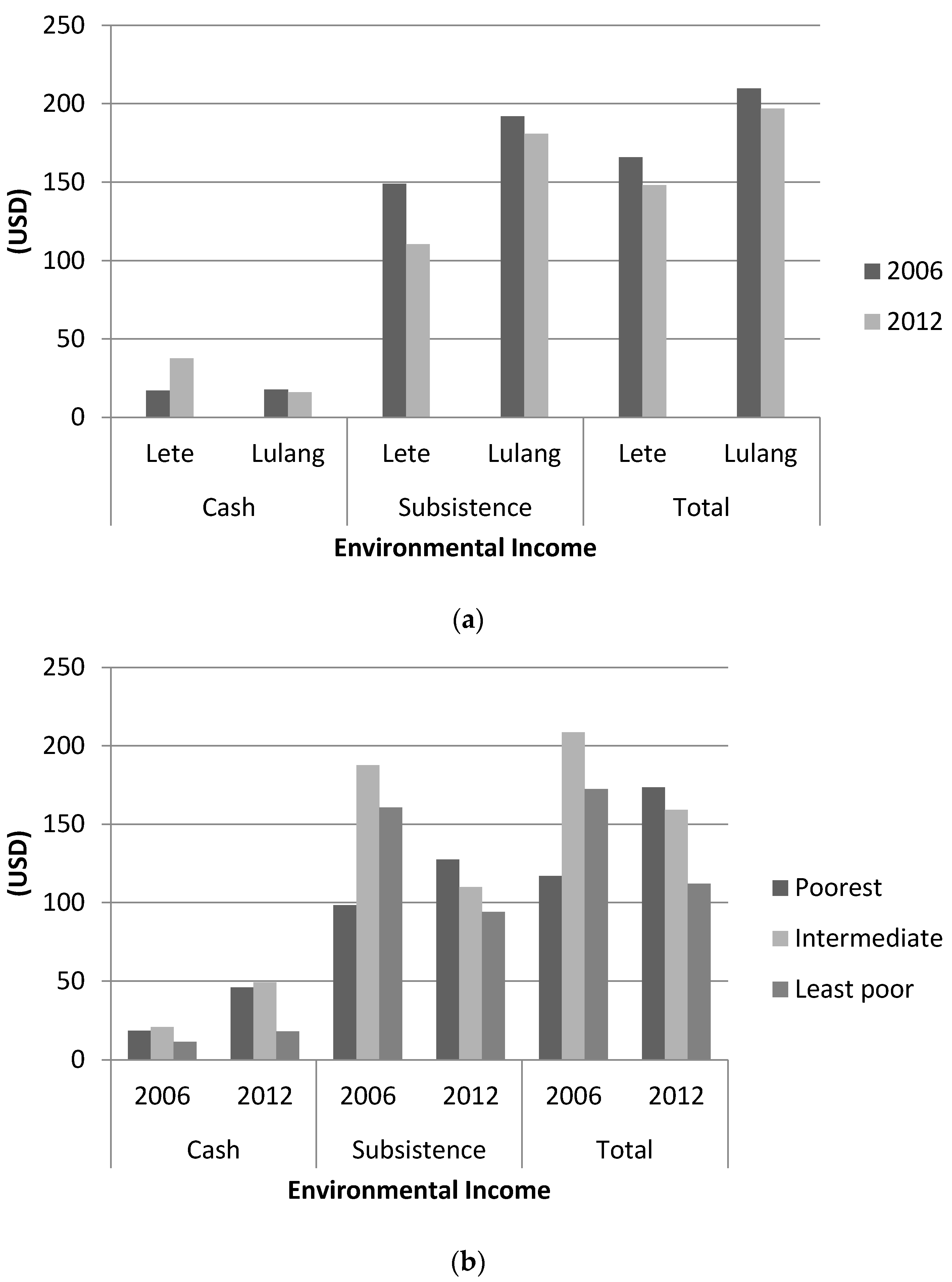[52] in their assessment of two wetland-situated villages in Trinidad and Tobago, where households without access to proper roads received much lower incomes for their products. Households in Lete are thus becoming more engaged in the market economy, selling more environmental products and reducing their use in home consumption. Contrary to the expectation that this change is driven by better off households, able to invest in bringing products to markets, we recorded the bulk of the increase in cash environmental income among poorer households (Figure 3b). Charlery et al. [17] found that increased environmental income in Lete contributed to decreasing income inequality. Additionally, if the increased trading of environmental products for cash is sustained, it is likely to have implications for rural households’ welfare dynamics, as the extraction of environmental resources can now directly contribute to asset accumulation, improving households’ chance of making a structural shift out of poverty [53]. Previous studies have focused on the role of environmental income in supporting current consumption and in providing safety-nets in response to shocks [4,14]. However, improved road infrastructure may also allow environmental income to contribute to asset accumulation.

Household characteristics positively associated with environmental income are those that support the willingness and ability of households to participate in environmental resource collection: labor availability, proximity of the household to forest and area of land holdings (owned or managed through rent). The participation of children and elders in the collection of environmental resources (such as firewood, leaf litter, wild fruits and vegetables) is common throughout rural Nepal. The dependency ratio therefore also appears as a significantly positive determinant of environmental income. Fisher and Shively [54] also found households with a higher dependency ratio to exhibit higher levels of forest extraction. The effect of the new road on environmental income is increased by a higher dependency ratio, possibly because environmental products can now more easily be sold for cash, making collection more attractive to households with excess low skill labor. This result is opposite to the findings of Viet Quang and Nam Anh [55], who found that households with a higher dependency ratio benefited less from the sale of non-timber forest products in Vietnam, but this variation can be due to the difference in context between the studies.

The location of the household is an indicator of the time required for household members to travel to and from environmental resource pools. Households residing closer to forests are able to gather greater quantities of environmental resources as also reported by McElwee [7] and Gunatilake [47]. However, the location of the household has no significant modifying effect on the impact of the road on environmental income, meaning that households in close proximity to forests did not increase their forest extraction activities more than those located at greater distances.

The area of land owned and managed by the household is an important determinant of environmental income, whether it is cultivated or uncultivated. This relates to the importance of forest leaf litter for the production of organic fertilizer used to maintain soil fertility [44,45]. Households owning uncultivated land have a private source of environmental resources, making it easier to collect higher quantities. Uncultivated lands are normally fallow land, steep sloping shrub lands, grass lands and primary forest, which in most cases cannot be cultivated. The effect of the road on environmental income is significantly and positively affected by an increase in the area of cropland owned and land rented by a household. More cropland means greater crop production and need for more environmental resources to maintain land fertility. However, the area of uncultivated land owned by the household has the opposite moderating effect on the impacts of the road on environmental income, perhaps indicating that these households are more engaged in new opportunities offered by the road and, thus, have less labor available to gather environmental resources or to cultivate their land.

On the other hand, we observed that households with a higher value of implements had lower environmental income. These households are more engaged in other income-generating activities related to the implements they own, such as private businesses, including processing of grains to produce alcohol, tailors/seamstresses and transportation, and, therefore, focus less on gathering environmental resources. Additionally, a higher value of implements reduced the road impacts on environmental income. This indicates that households, who initially earned less environmental income, because they were more engaged in other activities, further reduced the effort invested in this sector possibly due to further business opportunities offered by the new road.

4.2. Rural Roads and Environmental Reliance

The time trend showed that households in the study area generally became more reliant on the environment. However, the road reduced this trend in Lete. Unlike its impacts on environmental income, the new road had a significant negative impact on environmental reliance. This result was expected as new economic opportunities became available due to the road, e.g., as villagers incurred lower transportation costs for products to Beni and Jomsom, where there is also higher demand for skilled and unskilled labor. Although the increase in average wage income was not significant, it is possible that this demand for labor (source of additional wage income) has been captured in the category “other income”, which shows a highly significant increase. A limitation of the dataset is that during the process of data collection, households were not asked to identify the exact sources of other income, and this could have led to income from some forms of labor being reported as other income. Therefore, while households have the option of earning more cash income from environmental resources, they can also participate in new income-generating opportunities, making them less reliant on environmental income. Moreover, the impact of the road on environmental reliance was significantly and positively affected by the value of implements and the level of debt of the household. Households with a higher value of implements exhibit lower levels of environmental reliance, and with the new road, they are able to increase their earnings from other income-generating activities, thus further reducing their environmental reliance.

Studies have found that a higher level of education increases options for employment, and this results in households opting for more remunerative opportunities (when available) than environmental resource extraction [15,44], making them less environmentally reliant. Our results support these findings, although household head education level had no significant modifying effect on the impacts of the road on environmental reliance, perhaps because well-educated households already are less likely to be involved in environmental extraction activities [11].

Households with a higher dependency ratio have relatively fewer members who can gain employment in other income-generating activities. However, as explained above, these “unemployed” members contribute to the generation of environmental income, and this combined with lower income from other sources increases the households’ environmental reliance, thus appearing as a significant covariate in Table 3.

Similar to the findings by Rayamajhi et al. [11], our results show that higher debt increases environmental reliance, suggesting that indebted households resort to increased extraction of environmental resources to service their debt. A study by Gunatilake [47] hypothesized that indebted households are normally poorer, lacking endowments and, therefore, rely strongly on environmental resources. In our sample, the average debt to total income ratio was highest for households from the poorest income tercile, making this explanation plausible. However, an alternative explanation could be that higher debt means that these households have access to credit, which is invested in other activities—such as private businesses, farming and livestock production—in turn reducing environmental reliance [56]. Nonetheless, our results suggest that the former is the more likely explanation. The negative modifying effect of household debt on the effects of the road on environmental reliance suggests that these households resort to environmental resource extraction to service their debt only in the absence of more remunerative options.

4.3. Forest Conservation before and after Road Construction

Generally, road construction in remote, inaccessible areas presents threats of forest degradation and deforestation. Results from the forest inventories in Lete show that the rate of forest increment is significantly higher than the rate of extraction from 2005 (before the road) to 2010 (after the road). These inventories provide valuable information on the increment and extraction of wood-based forest products, such as fuelwood, poles and timber for construction. Although environmental income is generated from a wider range of environmental products than these, they constitute important products and can be used as indicators of the state of forest conservation in the area. Therefore, based on these measures, it appears that efforts aimed at forest conservation in Lete are effective, even with increased access to markets provided by the new road. This may reflect the generally conservative harvest levels in community forests also noted elsewhere in Nepal [57]. As it stands, even if households are allowed to triple their rate of extraction, this will not jeopardize the state of the forests. Note, however, that the inventories do not allow us to report on non-timber forest products, such as medicinal plants, and whether these are subjected to over-harvesting following road establishment. Though, judging from the household environmental income data, this is not likely to be the case. Nevertheless, it is important to note that given the short period between road construction and the second round of inventories, road impacts on the results might be limited, as changes in households’ activity patterns may take longer to produce measurable impacts.

5. Conclusions

The results of this study confirm the importance of environmental income to rural households in the Central Himalayan region of Nepal. Contributing an average of 29% in 2006 and 30% in 2012 to total household income in the two study sites, environmental income is more important than agricultural income from crop and livestock production. Policies and interventions aimed at improving the livelihoods of local people through the maximization of income opportunities thus need to account for environmental income as a major source of income in the region. Hence, policies directed towards reducing poverty also need to ensure the sustainable use of environmental resources.

Remote rural villages are increasingly connected to urban town centers through the construction of new roads. This study found significant positive impacts on household-level environmental income, while their environmental reliance decreased significantly. Although households increased their environmental income as a result of the road, they did not become more environmentally reliant, possibly because the road also provided access to other income-generating activities. Households became more market integrated, reducing subsistence consumption and increasing cash sales of environmental products, increasing the ability of this income source to contribute to household asset accumulation. This is an important aspect in relation to household welfare dynamics, which could be the focus of future studies.

Using plots to monitor forest stocks, we found that establishment of the road has not led to the harvest of wood products beyond increment levels, even to the extent that extraction levels can be increased with the associated local economic benefits. This indicates that forest conservation strategies in Lete, part of the Annapurna Conservation Area, are effective, even after the construction of the new road, or that environmental resource extraction is not economically competitive with other income-generating activities now available. Nonetheless, a follow-up round of inventories will provide a more accurate picture, as the time between the road construction and the second round may have been too short for providing long-term conclusions. However, so far, the results of this study suggest to environmental resource managers and development practitioners that infrastructural development can be achieved without negative consequences of excessive and unsustainable environmental exploitation while having positive overall welfare effects in terms of total household income.

References

1. Ellis, F. Rural Livelihoods and Diversity in Developing Cuntries; Oxford University Press: New York, NY, USA, 2000. [Google Scholar]
2. Winters, P.; Davis, B.; Carletto, G.; Covarrubias, K.; Quiñones, E.J.; Zezza, A.; Azzarri, C.; Stamoulis, K. Assets, activities and rural income generation: Evidence from a multicountry analysis. World Dev. 2009, 37, 1435–1452. [Google Scholar] [CrossRef]
3. Nielsen, Ø.J.; Rayamajhi, S.; Uberhuaga, P.; Meilby, H.; Smith-Hall, C. Quantifying rural livelihood strategies in developing countries using an activity choice approach. Agric. Econ. 2013, 44, 57–71. [Google Scholar] [CrossRef]
4. Angelsen, A.; Jagger, P.; Babigumira, R.; Belcher, B.; Hogarth, N.J.; Bauch, S.; Börner, J.; Smith-Hall, C.; Wunder, S. Environmental income and rural livelihoods: A global-comparative analysis. World Dev. 2014, 64, S12–S28. [Google Scholar] [CrossRef] [Green Version]
5. Cavendish, W. Quantitative method for estimating the Economic value of resource use to rural households. In Uncovering the Hidden Harvest; Campbell, B.M., Luckert, M.K., Eds.; Earthscan: London, UK, 2002; pp. 17–32. [Google Scholar]
6. Vedeld, P.; Angelsen, A.; Bojö, J.; Sjaastad, E.; Kobugabe Berg, G. Forest environmental incomes and the rural poor. For. Policy Econ. 2007, 9, 869–879. [Google Scholar] [CrossRef]
7. McElwee, P.D. Forest environmental income in Vietnam: Household socioeconomic factors influencing forest use. Environ. Conserv. 2008, 35, 147–159. [Google Scholar] [CrossRef]
8. Babulo, B.; Muys, B.; Nega, F.; Tollens, E.; Nyssen, J.; Deckers, J.; Mathijs, E. The economic contribution of forest resource use to rural livelihoods in Tigray, Northern Ethiopia. For. Policy Econ. 2009, 11, 109–117. [Google Scholar] [CrossRef]
9. Uberhuaga, P.; Smith-Hall, C.; Helles, F. Forest income and dependency in lowland Bolivia. Environ. Dev. Sustain. 2012, 14, 3–23. [Google Scholar] [CrossRef]
10. Mamo, G.; Sjaastad, E.; Vedeld, P. Economic dependence on forest resources: A case from Dendi District, Ethiopia. For. Policy Econ. 2007, 9, 916–927. [Google Scholar] [CrossRef]
11. Rayamajhi, S.; Smith-Hall, C.; Helles, F. Empirical evidence of the economic importance of Central Himalayan forests to rural households. For. Policy Econ. 2012, 20, 25–35. [Google Scholar] [CrossRef]
12. Hogarth, N.J.; Belcher, B.; Campbell, B.; Stacey, N. The role of forest-related income in household economies and rural livelihoods in the border-region of Southern China. World Dev. 2013, 43, 111–123. [Google Scholar] [CrossRef]
13. Prado Córdova, J.P.; Wunder, S.; Smith-Hall, C.; Börner, J. Rural income and forest reliance in highland Guatemala. Environ. Manag. 2013, 51, 1034–1043. [Google Scholar] [CrossRef] [PubMed]
14. Wunder, S.; Börner, J.; Shively, G.; Wyman, M. Safety nets, gap filling and forests: A global-comparative perspective. World Dev. 2014, 64, S29–S42. [Google Scholar] [CrossRef] [Green Version]
15. Fisher, M. Household welfare and forest dependence in Southern Malawi. Environ. Dev. Econ. 2004, 9, 135–154. [Google Scholar] [CrossRef]
16. Shackleton, C.M.; Shackleton, S.E.; Buiten, E.; Bird, N. The importance of dry woodlands and forests in rural livelihoods and poverty alleviation in South Africa. For. Policy Econ. 2007, 9, 558–577. [Google Scholar] [CrossRef]
17. Charlery, L.C.; Qaim, M.; Smith-Hall, C. Impact of infrastructure on rural household income and inequality in Nepal. J. Dev. Eff. 2016, 8, 266–286. [Google Scholar] [CrossRef]
18. Olsson, J. Improved road accessibility and indirect development effects: Evidence from rural Philippines. J. Transp. Geogr. 2009, 17, 476–483. [Google Scholar] [CrossRef]
19. Amadi, B.C. The impact of rural road construction on agricultural development: An empirical study of Anambra State in Nigeria. Agric. Syst. 1988, 27, 1–9. [Google Scholar] [CrossRef]
20. Isgut, A. Non-farm income and employment in rural Honduras: Assessing the role of locational factors. J. Dev. Stud. 2004, 40, 59–86. [Google Scholar] [CrossRef]
21. Warr, P. How road improvement reduces poverty: The case of Laos. Agric. Econ. 2008, 39, 269–279. [Google Scholar] [CrossRef]
22. Forman, R.; Alexander, L. Roads and their major ecological effects. Annu. Rev. Ecol. Syst. 1998, 29, 207–231. [Google Scholar] [CrossRef]
23. Angelsen, A.; Kaimowitz, D. Rethinking the causes of deforestation: Lessons from economic models. World Bank Res. Obs. 1999, 14, 73–98. [Google Scholar] [CrossRef] [PubMed]
24. Trombulak, S.C.; Frissell, C.A. Review of ecological effects of roads on terrestrial and aquatic communities and of aquatic ecological effects of roads on terrestrial commnunities. Conserv. Biol. 2000, 14, 18–30. [Google Scholar] [CrossRef]
25. Perz, S.G.; Caldas, M.M.; Arima, E.; Walker, R.J. Unofficial road building in the Amazon: Socioeconomic and biophysical explanations. Dev. Chang. 2007, 38, 529–551. [Google Scholar] [CrossRef]
26. Poulsen, J.R.; Clark, C.J.; Mavah, G.; Elkan, P.W. Bushmeat supply and consumption in a tropical logging concession in northern Congo. J. Soc. Conserv. Biol. 2009, 23, 1597–1608. [Google Scholar] [CrossRef] [PubMed]
27. Sudmeier-Rieux, K.; Jaquet, S.; Derron, M.-H.; Jaboyedoff, M.; Devkota, S. A case study of coping strategies and landslides in two villages of Central-Eastern Nepal. Appl. Geogr. 2012, 32, 680–690. [Google Scholar] [CrossRef]
28. Adam, M.; Kneeshaw, D.; Beckley, T. Forestry and road development: Direct and indirect impacts from an aboriginal perspective. Ecol. Soc. 2012, 17, 1–13. [Google Scholar] [CrossRef]
29. Laurance, W.F.; Clements, G.R.; Sloan, S.; O’Connell, C.S.; Mueller, N.D.; Goosem, M.; Venter, O.; Edwards, D.P.; Phalan, B.; Balmford, A.; et al. A global strategy for road building. Nature 2014, 513, 229–232. [Google Scholar] [CrossRef] [PubMed]
30. Barber, C.P.; Cochrane, M.A.; Souza, C.M.; Laurance, W.F. Roads, deforestation, and the mitigating effect of protected areas in the Amazon. Biol. Conserv. 2014, 177, 203–209. [Google Scholar] [CrossRef]
31. Baraloto, C.; Alverga, P.; Quispe, S.B.; Barnes, G.; Chura, N.B.; da Silva, I.B.; Castro, W.; da Souza, H.; de Souza Moll, I.E.; et al. Effects of road infrastructure on forest value across a tri-national Amazonian frontier. Biol. Conserv. 2015, 191, 674–681. [Google Scholar] [CrossRef]
32. Bhattarai, K.; Conway, D.; Yousef, M. Determinants of deforestation in Nepal’s Central Development Region. J. Environ. Manag. 2009, 91, 471–488. [Google Scholar] [CrossRef] [PubMed]
33. Van De Walle, D. Choosing rural road investments to help reduce poverty. World Dev. 2002, 30, 575–589. [Google Scholar] [CrossRef]
34. Fan, S.; Chan-Kang, C. Regional road development, rural and urban poverty: Evidence from China. Transp. Policy 2008, 15, 305–314. [Google Scholar] [CrossRef]
35. Khandker, S.; Bakht, Z.; Koolwal, G. The poverty impact of rural roads: Evidence from Bangladesh. Econ. Dev. Cult. Chang. 2009, 57, 685–722. [Google Scholar] [CrossRef]
36. Gibson, J.; Olivia, S. The effect of infrastructure access and quality on non-farm enterprises in rural Indonesia. World Dev. 2010, 38, 717–726. [Google Scholar] [CrossRef]
37. Rand, J. Evaluating the employment-generating impact of rural roads in Nicaragua. J. Dev. Eff. 2011, 3, 28–43. [Google Scholar] [CrossRef]
38. Angelsen, A.; Larsen, H.O.; Lund, J.F.; Smith-Hall, C.; Wunder, S. Why measure rural livelihoods and environmental dependence? In Measuring Livelihoods and Environmental Dependence: Methods for Research and Fieldwork; Angelsen, A., Larsen, H.O., Lund, J.F., Smith-Hall, C., Wunder, S., Eds.; Earthscan: London, UK, 2011; pp. 1–16. [Google Scholar]
39. Krishna, A. Escaping poverty and becoming poor: Who gains, who loses, and why? World Dev. 2004, 32, 121–136. [Google Scholar] [CrossRef]
40. Kristjanson, P.; Krishna, A.; Radeny, M.; Kuan, J.; Quilca, G.; Sanchez-Urrelo, A.; Leon-Velarde, C. Poverty dynamics and the role of livestock in the Peruvian Andes. Agric. Syst. 2007, 94, 294–308. [Google Scholar] [CrossRef]
41. Wunder, S.; Luckert, M.; Smith-Hall, C. Valuing the priceless: What are non-marketed products worth? In Measuring Livelihoods and Environmental Dependence: Methods for Research and Fieldwork; Angelsen, A., Larsen, H.O., Lund, J.F., Smith-Hall, C., Wunder, S., Eds.; Earthscan: London, UK, 2011; pp. 127–145. [Google Scholar]
42. Müller, W.G. Collecting Spatial Data: Optimum Design of Experiments for Random Fields; Physica-Verlag: Heidelberg, Germany, 2001. [Google Scholar]
43. Meyer, B. Natural quasi-experiments in economics. J. Bus. Econ. Stat. 1995, 13, 151–161. [Google Scholar]
44. Adhikari, B.; Di Falco, S.; Lovett, J.C. Household characteristics and forest dependency: Evidence from common property forest management in Nepal. Ecol. Econ. 2004, 48, 245–257. [Google Scholar] [CrossRef]
45. Adhikari, B. Poverty, property rights and collective action: Understanding the distributive aspects of common property resource management. Environ. Dev. Econ. 2005, 10, 7–31. [Google Scholar] [CrossRef]
46. Adhikari, M.; Nagata, S.; Adhikari, M. Rural household and forest: An evaluation of household’s dependency on community forest in Nepal. J. For. Res. 2004, 9, 33–44. [Google Scholar] [CrossRef]
47. Gunatilake, H. The role of rural development in protecting tropical rainforests: Evidence from Sri Lanka. J. Environ. Manag. 1998, 53, 273–292. [Google Scholar] [CrossRef]
48. Sharma, E.R.; Pukkala, T. Volume Tables for Forest Trees of Nepal; Ministry of Forests and Soil Conservation, Forest Survey and Statistics Division, HMG/Nepal: Kathmandu, Nepal, 1990; Volume 48. [Google Scholar]
49. Metz, J. Forest product use at an upper elevation village in Nepal. Environ. Manag. 1994, 18, 371–390. [Google Scholar] [CrossRef]
50. Dillon, A.; Sharma, M.; Zhang, X. Estimating the impact of rural investments in Nepal. Food Policy 2011, 36, 250–258. [Google Scholar] [CrossRef]
51. Biggs, E.; Watmough, G. A community-level assessment of factors affecting livelihoods in Nawalparasi District, Nepal. J. Int. Dev. 2011, 24, 255–263. [Google Scholar] [CrossRef]
52. Shah, K.U.; Dulal, H.B.; Johnson, C.; Baptiste, A. Understanding livelihood vulnerability to climate change: Applying the livelihood vulnerability index in Trinidad and Tobago. Geoforum 2013, 47, 125–137. [Google Scholar] [CrossRef]
53. Barrett, C.B. Rural poverty dynamics: Development policy implications. Agric. Econ. 2005, 32, 45–60. [Google Scholar] [CrossRef]
54. Fisher, M.; Shively, G. Can income programs reduce tropical forest pressure? Income shocks and forest use in Malawi. World Dev. 2005, 33, 1115–1128. [Google Scholar] [CrossRef]
55. Viet Quang, D.; Nam Anh, T. Commercial collection of NTFPs and households living in or near the forests. Case study in Que, Con Cuong and Ma, Tuong Duong, Nghe An, Vietnam. Ecol. Econ. 2006, 60, 65–74. [Google Scholar] [CrossRef]
56. Dev, O.; Yadav, N.; Springate-Baginski, O.; Soussan, J. Impacts of community forestry on livelihoods in the middle hills of Nepal. J. For. Livelihood 2003, 3, 64–77. [Google Scholar]
57. Meilby, H.; Smith-Hall, C.; Byg, A.; Larsen, H.O.; Nielsen, Ø.J.; Puri, L.; Rayamajhi, S. Are forest incomes sustainable? Firewood and timber extraction and productivity in community managed forests in Nepal. World Dev. 2014, 64, 113–124. [Google Scholar] [CrossRef]
Figure 1. Map of Nepal showing Lete and Lulang Village Development Committees (VDCs).
Sustainability 08 00363 g001
Figure 2. Map of Lete showing the seven forest strata (S.1–S.7).
Sustainability 08 00363 g002
Figure 3. (a) Cash and subsistence EI (USD per AEU) in Lete and Lulang VDCs in 2006 and 2012; (b) cash and subsistence EI by wealth terciles (USD per AEU) in Lete in 2006 and 2012.
Sustainability 08 00363 g003