Abstract
Cycling accessibility is a key indicator of urban resource equity and built environment performance. However, its relationship with equity, the importance of built environment factors, and nonlinear effects across facility types remain underexplored. This study combines the Gini coefficient with a generalized additive model (GAM) to examine the nonlinear accessibility–equity relationship and uses Light Gradient Boosting Machine (LightGBM) with SHapley Additive exPlanations (SHAP) to assess the importance and nonlinear effects of built environment variables. Potential effects of vegetation (Normalized Difference Vegetation Index, NDVI) and precipitation are also explored. Results show that both accessibility and equity peak in urban cores and decline toward peripheral areas. Facility types exhibit distinct patterns: accommodation services have high accessibility but low equity, life services require higher accessibility to achieve equity, and public services show an N-shaped relationship. SHAP analyses indicate that traffic signals, subway station accessibility, and street enclosure ratio are associated with higher cycling accessibility, whereas a higher sky view index is associated with lower accessibility. Observed moderating effects of vegetation and precipitation provide further insights into potential interactions. These findings offer guidance for improving cycling infrastructure and promoting more equitable and sustainable urban accessibility.
1. Introduction
Bicycle travel, with low cost, low emissions, and health benefits [1], has become an important mode for medium- and short-distance trips and a key connection to rail transit. Yet, promoting cycling faces multiple challenges, especially equity issues [2]. Accessibility, a central topic in urban science, influences land rent, population distribution [3], economic development, and spatial inequality [4]. In cycling, accessibility is a crucial indicator, with significant spatial disparities across functional services [5]. Built environment factors directly affect cycling accessibility, and uneven distribution may create disparities in cycling opportunities, raising equity concerns [6]. Exploring these effects thus has theoretical and practical significance.
Previous studies on the built environment primarily focused on its effects on cycling behavior, commonly used indicators such as land-use type, population density, bicycle infrastructure, bus stop density, and roadside greenery [7,8]. With the advancement of research, variables such as land-use mix, accessibility, and environmental aesthetics were also demonstrated to exert significant influences on transport-related cycling [9]. In addition, demographic characteristics, residential preferences, and travel attitudes were often incorporated as control variables in analytical frameworks [10]. At the facility level, different types of cycling infrastructure (e.g., bicycle lanes and bicycle paths) were found to exert differentiated impacts on public bicycle use [11], while high-density land use tended to promote bike-sharing activities; conversely, longer distances to metro stations and greater lengths of greenways might have had negative effects [12]. In recent years, studies increasingly incorporated cyclists’ subjective perceptions—such as sky view index, green view index, and street interface features—into analytical models, which revealed their critical roles in shaping shared bicycle use [13,14].
Accessibility, one of the key dimensions of the built environment, is defined as the ability of individuals to reach activity locations, interact with others, or utilize various opportunities [15]. In cycling research, accessibility is typically measured by spatial distance, where greater distance indicates lower accessibility [16]. Common quantitative indicators include the distance to the nearest opportunity point, the number of opportunities within a given distance or time threshold, the average distance to all opportunities, and the mean distance to several nearest opportunities [17]. In this study, the cumulative opportunity method [18] was adopted using the number of accessible facilities within a defined distance range along the road network to measure cycling accessibility. This approach was chosen for its maturity, simplicity, and effectiveness in evaluating residents’ cycling accessibility within specific distance ranges during daily travel [5].
A growing body of research demonstrates that the built environment exerts a significant influence on cycling accessibility [19]. For example, the addition of sidewalks and bicycle lanes in communities enhanced cycling levels, while integrating cycling with public transportation not only promoted active travel [20] but also significantly improved job accessibility [21]. Cycling accessibility was affected not only by individual characteristics but also by environmental conditions, among which the expansion and increased density of bicycle lane networks markedly improved travel accessibility [22]. Moreover, accessibility exhibited substantial perceptual differences shaped by multiple factors, including infrastructure conditions, travel habits, and environmental characteristics [23].
Previous studies on cycling accessibility equity mainly used linear models to analyze differences among groups such as children, older adults, and individuals of varying gender and income [2,24]. Findings showed that facilities were often concentrated in central areas with higher socio-economic populations [25]. Although bicycle networks expanded, ordinary least squares (OLS) and logistic regression indicated limited accessibility improvements for vulnerable groups. Recently, mixed-effects models have been adopted to better capture relationships between socio-demographics and bicycle lane variables [26]. Lorenz curves and Gini coefficients are widely used to assess equity, and this study follows this approach. For instance, studies in Bogotá [5] and bike-sharing systems [27] revealed significant disparities in access and facility distribution among socio-economic groups.
Nevertheless, research on the built environment remains largely fragmented, lacking systematic comparative analyses of the relative importance of infrastructural and perceptual factors within an integrated framework. Most studies also fail to identify the direct effects of the built environment on cycling while adequately controlling for demographic and natural environmental factors. In addition, accessibility and equity research still relies predominantly on linear approaches, focuses mainly on population-based disparities, and pays limited attention to spatial heterogeneity in cycling accessibility and its intrinsic link with equity. Systematic examination of the nonlinear mechanisms through which the built environment influences cycling accessibility across different facility types is absent.
To address the existing research gaps, this study aims to systematically reveal the characteristics of urban cycling accessibility and its equity, and to examine the key roles of built environment variables. By quantifying cycling accessibility and equity across different types of functional facilities, the study innovatively uncovers the spatial coupling patterns and corresponding relationships, such as “high accessibility–low equity” modes. While accounting for natural environmental variables and population, the analysis focuses on the associations of built environment variables and their nonlinear patterns and examines potential moderation by natural variables. The findings provide insights into urban cycling environments and the spatial distribution of public facilities, potentially supporting carbon reduction and sustainable urban development. The remainder of the paper is organized as follows. Section 2 introduces the study area, data, and methods, including Gini coefficient calculation and modeling approaches. Section 3 presents the results. Section 4 discusses the findings and policy implications, and Section 5 concludes the study.
2. Materials and Methods
2.1. Research Framework
The study framework includes three parts: data collection, methodology, and results analysis (Figure 1). The study focused on Xi’an’s central urban area, collecting data on the urban road network, four types of functional service points, 15 built environment variables, and control variables. Cycling accessibility was measured using the cumulative opportunities approach, and equity was evaluated with the Gini coefficient. GAM analyzed spatial relationships between accessibility and equity, while LightGBM assessed built environment effects and SHAP interpreted the model results. Results analysis examined spatial patterns of accessibility and equity across facility types, key built environment variables affecting accessibility, and interactions with natural factors to explain disparities.
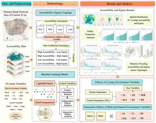
Figure 1.
Research framework.
2.2. Study Area
Xi’an, the largest city in Northwest China [28], serves as the focus of this study, which specifically investigates the main urban area, encompassing 58 subdistricts and covering a total area of 846.54 km2 (Figure 2). According to statistical data, the permanent population of Xi’an’s central urban area reached 7.1967 million in 2020 [29]. The area is characterized by relatively high bicycle usage [30] and extensive street view coverage. To obtain the most comprehensive street view data, the outermost boundaries of the study area were delineated based on village or community units. However, because these units are relatively small and inconvenient for visualization and spatial analysis, the maps present the study area at the subdistrict level. It should be noted that some peripheral areas may not correspond to complete subdistrict offices. Additionally, to ensure continuity of the road network, Fengdong Subdistrict of Xianyang City, which crosses administrative boundaries, was included in the cycling accessibility calculation, but this area was excluded from subsequent analyses.
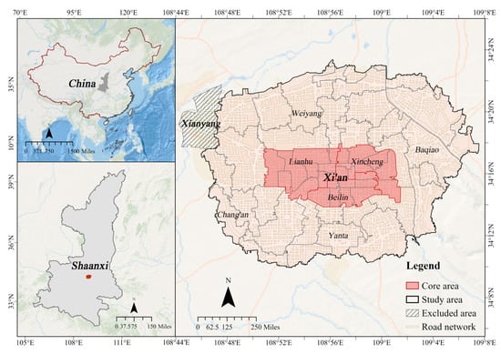
Figure 2.
Study area and location map.
2.3. Cycling Accessibility Calculation
To systematically assess the accessibility of functional service points for cycling, data on a total of 11 types of functional service points in Xi’an in 2023 were obtained from the Gaode map API. Following relevant literature [31,32,33] and considering the attributes of each facility type in terms of residents’ daily life, access to public services, and leisure preferences, the raw data were reclassified into four categories (Table 1) to comprehensively reflect the spatial distribution of urban functions.

Table 1.
Functional service point classification and type composition.
The urban road network data were derived from the cycling network in OpenStreetMap (OSM) and were further adjusted to reflect the actual conditions of the study area, resulting in a topological road network model encompassing arterial roads, secondary roads, and selected local streets. Given the high permeability of bicycle networks [34], and the lack of clearly defined entry and exit points, sampling points were generated along the roads at 200 m intervals in ArcGIS 10.8.1, yielding 28,850 points, which were used as spatial analysis units. Subsequently, cycling accessibility from each sampling point was calculated using the Network Analyst extension [5,25]. Following block-level studies [2], a 1000 m radius (approximately 5 min cycling) was adopted to compute the number of accessible functional service points within this range for each sampling point. Finally, the accessibility results were aggregated into 500 m × 500 m fishnet grids based on the total count, creating the spatial dataset used in subsequent machine learning analyses.
2.4. Variable Selection
2.4.1. Built Environment Variables
This study selected 10 built environment variables covering bicycle infrastructure, cycling comfort, and public transit accessibility (Table 2). Six variables, including bicycle lane density (BLD), bicycle lane barrier density (BLB), number of bicycle racks (BR), green view index (GVI), sky view index (SVI), and street enclosure ratio (SER), were extracted from Baidu Maps Street View images at 200 m intervals. Street view images were obtained from Baidu Maps’ real-time updates, representing the urban environment as of 2023. Over 25,000 panoramic images were segmented using Mask2Former with the Mapillary dataset to extract urban elements (Figure S1).
Table 2.
Indicator system and descriptions.
In addition, subway stations and bus stops in Xi’an in 2023 were obtained via the Gaode Maps API. Subway station accessibility (SS) was measured as the number of subway stations reachable within a 1000 m cycling distance from each sampling point. Due to their smaller service area, bus stop accessibility (BS) was calculated as the number of bus stops reachable within a 500 m cycling distance (approximately 3 min) [25], using the same method applied for functional service point accessibility. GVI, SVI, and SER were aggregated as grid averages, while all other variables were summed within each grid, generating a spatial dataset for subsequent machine learning analyses.
2.4.2. Control Variables
To effectively control for the potential confounding effects of natural factors and population on the relationship between built environment variables and cycling accessibility, five representative variables were selected [35,36,37]: temperature, precipitation, Normalized Difference Vegetation Index (NDVI), PM2.5 concentration, and population. These variables reflect regional climate comfort, weather conditions, vegetation coverage, air quality, and population distribution, all of which may influence residents’ travel preferences and cycling behavior, thereby indirectly affecting cycling accessibility.
Natural factor data for 2023 were obtained from the official website of the Chinese National Qinghai–Tibet Plateau Scientific Data Center, with an original spatial resolution of 30 m. Population data for 2023 were sourced from dataset [38], with an original resolution of 100 m. To maintain consistency with the built environment variables, all data were spatially aggregated to 500 m × 500 m fishnet grids. Natural factors were averaged within each grid, while the population was summed. Spatial alignment across all grids was ensured during aggregation.
2.5. Methods
2.5.1. Gini Coefficient and Lorenz Curve
In 1912, Corrado Gini first proposed the Gini coefficient to measure inequality among N quantities, which was widely applied in income distribution studies [39]. The Gini coefficient quantifies the Lorenz curve [40] to represent income distribution, where greater deviation of the curve from the line of perfect equality indicates higher inequality. In recent years, the Gini coefficient was increasingly applied in the transportation field to assess the spatial equity of accessibility to various service facilities [41,42]. Its calculation formula is as follows:
In this study, i represents a subdistrict in the central urban area of Xi’an, where i = 1, 2, 3, …, n; P denotes the total population of the central urban area; Pi represents the population of subdistrict i; and Bi indicates the cumulative proportion of cycling accessibility for subdistrict i. The Gini coefficient ranges from 0 (perfect equality) to 1 (extreme inequality).
We assessed the equity of cycling accessibility for four types of functional service points by calculating accessibility for each type and weighting it by the population of the corresponding subdistrict. At the global level, a single Gini coefficient was calculated for the entire study area based on the cumulative distribution of population-weighted accessibility, with the Lorenz curve representing overall facility equity. At the subdistrict level, Gini coefficients were computed using fishnet-based accessibility within each subdistrict, and these values were used for spatial visualization and GAM analysis. There is no universally accepted standard for interpreting Gini coefficient values in terms of equity. The United Nations Human Settlements Programme (UN-Habitat) suggests a widely recognized reference value, setting the “international alert line” at 0.4 [43]. Following relevant studies [44,45], four thresholds were defined in this study (Below 0.3, 0.3–0.4, 0.4–0.5, Over 0.5) to classify equity levels into four categories: “Equal,” “Relatively equal,” “Inequality,” and “High inequality.”
2.5.2. Generalized Additive Model (GAM)
The generalized additive model (GAM) is an extension of the generalized linear model (GLM) that allows nonlinear functions of independent variables to enter the model in an additive manner, providing a flexible generalization of GLM [46,47]. Its fitting typically relies on scatterplot smoothers, backfitting algorithms, and local scoring procedures [48]. In this study, GAM was employed to analyze the nonlinear relationships between subdistrict-level accessibility of different types of functional service points and their corresponding subdistrict-level equity. The model is expressed as follows:
yi represents the equity indicator of subdistrict i, corresponding to one of the four functional service point types: LifeS, PubS, ResS, or AccS; denotes the corresponding single accessibility indicator for LifeS, PubS, ResS, or AccS; is a nonparametric smoothing function used to capture the nonlinear effect of the independent variable on the equity indicator; and is the error term. We used the pyGAM library in Python 3.10 to perform univariate fitting for each accessibility indicator and its corresponding equity indicator, revealing their independent contributions and nonlinear trends, thereby accurately reflecting the relationship between accessibility and equity within the study area.
2.5.3. Light Gradient Boosting Machine (LightGBM)
This study employed the LightGBM algorithm, which showed higher training efficiency and scalability for high-dimensional features and large datasets compared with models such as XGBoost and pGBRT [49]. Continuous features were discretized into bins, and trees were constructed using a leaf-wise splitting strategy to enhance predictive accuracy [50].
During model training, several control variables (e.g., natural factors and population) were included to account for their potential influence on the dependent variable in the model. Both control variables and main independent variables were used as input features, allowing LightGBM to learn the relative contribution of each feature to predictive performance within a unified modeling framework. Accordingly, associations between the main independent variables and the dependent variable were examined in a multivariate context. In the output analysis, interpretation focused on the main independent variables, while control variables were not discussed separately. This approach aims to characterize conditional associations and nonlinear patterns rather than causal effects.
Hyperparameters were optimized through grid search with five-fold cross-validation. All parameter combinations were evaluated by randomly splitting the training set into five folds (80% training, 20% validation; KFold, shuffle = True, random_state = 42). The model was fitted on training folds, and R2 was calculated for training and validation sets. The average five-fold R2 was used to select the optimal hyperparameters, ensuring controlled differences between training and validation to reduce overfitting. Model performance was assessed using R2 and RMSE [50].
2.5.4. SHAP
Compared with traditional machine learning methods, interpretable machine learning can reveal the internal structure of models, thereby enhancing their interpretability [51]. Lundberg and Lee [52] proposed SHAP values and developed approximate algorithms to address computational challenges. Subsequently, Lundberg et al. [53] introduced the TreeExplainer method for tree-based models such as XGBoost and LightGBM. Based on this, the present study employed SHAP to analyze and visualize the contributions of built environment variables to the accessibility of different types of functional service points and further evaluated the interactive effects between built environment variables and natural factors on accessibility.
3. Results
3.1. Cycling Accessibility and Equity Results
3.1.1. Spatial Disparities in Cycling Accessibility and Equity
As shown in Figure 3 and Figure S2, significant differences in cycling accessibility and equity were observed among different types of functional service points. Overall, the Lorenz curves indicated that accessibility was generally unequal for all service types (GINI > 0.4). Accommodation services (AccS) exhibited the highest Gini coefficient (0.677), indicating the greatest overall inequity in cycling accessibility, with subdistricts of high inequality accounting for 65.5%, markedly higher than other types. The Gini coefficients of the other three service types were similar: 0.549 for public services (PubS), 0.527 for life services (LifeS), and 0.513 for residential services (ResS). Among them, PubS had a total 67.3% of subdistricts with inequality, with subdistricts of high inequality accounting for 39.7%, second only to AccS. LifeS showed a higher proportion of subdistricts with inequality (69%). ResS were relatively more evenly distributed (0.513), yet the total proportion of subdistricts with inequality still reached 68.9%. In summary, except for AccS, the Gini coefficients of the other three types were slightly lower, but the proportion of subdistricts with inequality remained high.
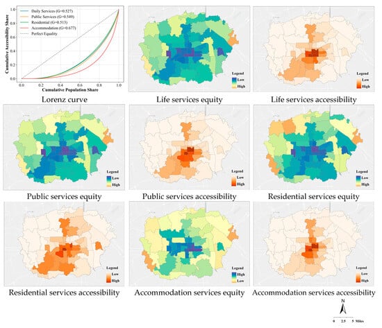
Figure 3.
Spatial visualization of cycling accessibility and equity.
As shown in Figure 3, all four facility types exhibited higher accessibility and relatively fair distribution in the urban core (Figure 2), whereas both accessibility and equity gradually declined toward peripheral areas. Life services (LifeS) and public services (PubS) showed similar spatial patterns: accessibility was highest in the core, relatively high and evenly distributed in the southwest and due north, and lowest in the northwest and east, accompanied by pronounced inequity. Residential services (ResS) displayed the highest equity in the core, with relatively high equity in the south and due north; however, accessibility was only favorable in the southwest and due north, while the northwest and east experienced generally low accessibility and low equity. Accommodation services (AccS) exhibited generally low accessibility and equity outside the urban core, with a clear spatial mismatch between the two.
3.1.2. Correlation Between Accessibility and Equity
As shown in Figure S3, the four types of service facilities generally exhibited consistent trends between accessibility and equity. Overall, subdistricts characterized by “low accessibility–low equity” accounted for over 45%, the highest proportion among the four facility types; this was followed by subdistricts of “high accessibility–high equity” and “high accessibility–low equity.”
Subdistricts of the “low accessibility–high equity” type were the least, all below 5%. Specifically, accommodation services (AccS) had markedly fewer subdistricts in the “high accessibility–high equity” category compared to the other three types, while the number of subdistricts in the “high accessibility–low equity” category was significantly higher than the other three types.
To further investigate the relationship between accessibility and equity, generalized additive models (GAM) were employed to fit the subdistrict-level accessibility and equity for the four types of functional service points (Figure S3). Specifically, life services (LifeS) subdistricts required an accessibility of approximately 4000 for the Gini coefficient to fall below 0.4; residential services (ResS) and accommodation services (AccS) required approximately 800 and 1100, respectively.
Public Services (PubS) exhibited a two-stage pattern, with equity reaching a higher level only when accessibility exceeded roughly 900 or 1900. Further analysis of the accessibility corresponding to peak equity revealed values of about 10,000 for LifeS, 2500 for PubS, and 1400 and 1500 for ResS and AccS, respectively. Overall, LifeS required the highest accessibility to achieve equitable distribution, while ResS required the lowest; the same pattern was observed at the equity peak. Notably, ResS and AccS included subdistricts with significantly high Gini coefficients, indicating extreme inequity in localized areas.
3.2. Effects of Built Environment Variables
3.2.1. Data Processing and Model Fitting Performance
Variance inflation factor (VIF) tests were conducted on the independent variables (Table S1). PM2.5, temperature (Temp), and precipitation (Prec) had VIFs > 10, with Temp highest at 36.47. After removing Temp, all remaining variables had VIFs below 10 (Table S2), indicating no significant multicollinearity [54], and suitability for regression. The processed data were input into LightGBM to model cycling accessibility for four service types. Training set R2 values were 0.877 (LifeS), 0.884 (PubS), 0.786 (ResS), and 0.647 (AccS); test set R2 values were 0.792, 0.808, 0.691, and 0.529, respectively Table S3. Overall, model performance was good, with PubS achieving the highest prediction accuracy and AccS the lowest.
3.2.2. Contribution of Built Environment Variables
This study analyzed the determinants of cycling accessibility for four types of service facilities using the LightGBM model combined with SHAP values (Figure 4). The results indicated that the number of traffic signals (TL), subway station accessibility (SS), street enclosure ratio (SER), sky view index (SVI), and number of road intersections (RI) consistently ranked among the top six influential variables across all facility types, while bus stop accessibility (BS) significantly affected the accessibility of life services (LifeS), public services (PubS), and residential services (ResS).
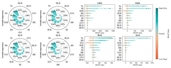
Figure 4.
Accessibility importance ranking and summary. (left) Shows the relative importance of built environment variables as a percentage; (right) shows the distribution of SHAP values and the direction of SHAP value clustering. More important variables tend to cluster in areas with higher SHAP values, indicating their greater influence on model prediction.
As shown in Figure 4, TL exhibited a consistently positive effect across all four facility types, contributing over 24% overall, with the highest contribution for accommodation services (AccS) at 27.4%, followed by PubS at 27.1%, and ResS and LifeS at around 25%. SS also showed strong effects, particularly on AccS (36.8%), and played an important role for LifeS and PubS as well. Both SER and SVI had notable impacts, though their influence varied by facility type: SER was strongest for LifeS (15%), whereas SVI had more pronounced effects on PubS (16.6%) and ResS (15.5%). In contrast, RI contributed relatively less across all facility types. BS had a limited overall effect, but its contribution reached 20.6% for ResS, highlighting its specific importance for residents’ daily accessibility.
3.2.3. Dependence Effects of Key Built Environment Variables
To eliminate the scale effects caused by differences in accessibility values across different facility types, the accessibility values were standardized using Z-scores in the single-factor dependence analysis, ensuring comparability across facility types. Based on this, the six key built environment variables mentioned above were further investigated.
The results indicated that, except for sky view index (SVI), all other built environment variables exerted positive effects on cycling accessibility across the four facility types (Figure 5). Specifically, the number of traffic signals (TL) had the most pronounced effect on life services (LifeS) accessibility, with the highest peak contribution; in contrast, its influence on accommodation services (AccS) and residential services (ResS) was relatively weaker, and marginal gains in accessibility diminished when the number of signals exceeded approximately 15. Subway station accessibility (SS) showed an overall significant positive effect, though the change was less pronounced for ResS and most prominent for AccS. Street enclosure ratio (SER) had the strongest impact on LifeS, exhibiting the largest fluctuation in dependency values, while its effect on AccS was minimal. Road intersection density (RI) displayed a similar pattern. Bus stop accessibility (BS) most substantially enhanced ResS accessibility, far exceeding its effects on other facility types, and was nearly ineffective for AccS. SVI exhibited a negative effect, particularly on public services (PubS) and ResS, with the adverse impact becoming especially evident when SVI exceeded 0.2.
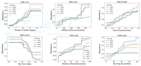
Figure 5.
Key built environment variables dependence plot. All dependence analyses were conducted at the fishnet grid level, with the X-axis representing values per 500 m × 500 m fishnet grid.
3.3. Moderating Effects of Natural Factors on Built Environment Variables
The moderating effects of natural factors on built environment variables were analyzed using the top three SHAP interactions per facility type (Figure 6). For LifeS, the strongest interactions were the interaction between NDVI and traffic signals (TL, 19.72), the interaction between NDVI and subway station accessibility (SS, 18.23), and the interaction between precipitation (Prec) and bus stop accessibility (BS, 18.16). For PubS, NDVI was the primary moderator: the interaction between NDVI and BS (8.67), NDVI and TL (6.93), and NDVI and green view index (GVI, 3.93). For ResS, precipitation dominated the interaction between Prec and BS (7.42) and Prec and TL (6.30). For AccS, the interaction between NDVI and SS (3.91) was strongest, followed by the interaction between Prec and SS and the interaction between NDVI and bicycle racks (BR). SHAP scatter plots (Figure 7) confirmed significant interactions of NDVI and Prec with key built environment variables (SS, TL) across facility types. The interaction between NDVI and SS positively influenced LifeS but negatively affected PubS and AccS when NDVI was around 0.3, reducing SHAP values by approximately 80. The interaction between Prec and SS increased AccS accessibility at annual precipitation of about 600 mm. The interaction between NDVI and TL slightly reduced accessibility for LifeS and PubS, whereas the interaction between Prec and TL increased accessibility for LifeS and ResS under approximately 600 mm precipitation. For ResS, the interaction between Prec and BS substantially improved accessibility, while higher SER slightly reduced it. Other notable interactions included the interaction between NDVI and GVI negatively affecting PubS and the interaction between NDVI and BR negatively affecting AccS.
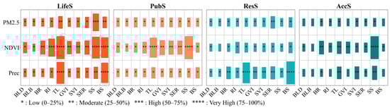
Figure 6.
Heatmap of interaction values between built environment variables and natural factors.
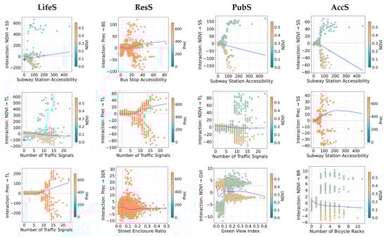
Figure 7.
Scatter plot of natural factors’ modulation of built environment effects on cycling accessibility. LOWESS curves were used to smoothly display the local trends of interactions between natural factors and built environment variables on cycling accessibility. These curves visually illustrate the positive or negative contributions of interactions to accessibility as built environment variables change, helping to identify the strength and direction of interaction effects across different facility types.
4. Discussion
4.1. Analysis of Cycling Accessibility and Equity
Cycling accessibility showed notable inequity (Gini > 0.4) across all four facility types. Core urban areas exhibited higher accessibility and equity, decreasing toward the periphery, consistent with previous studies [55]. Commercial accommodation facilities displayed the greatest inequity, with the highest proportion of high-inequity subdistricts. Outside the core, low accessibility–low equity was widespread, likely due to clustering of tourist and commercial areas disconnected from the cycling network. For the other three facility types, Gini coefficients were slightly lower, but over 67% of subdistricts still showed significant inequity. Accessibility was highest in the core, reflecting a better alignment of cycling networks and facility distribution in older districts. Indicators were also relatively high in the southwestern mature residential zone within the high-tech industrial park, where daily life, public service, and residential facilities are well distributed, and in the northern emerging sub-center, reflecting coordinated allocation of cycling infrastructure and services during urban expansion.
Regarding accessibility–equity correlations, subdistricts with “low accessibility–low equity” were the most common, followed by “high accessibility–high equity” and “high accessibility–low equity.” In general, low accessibility corresponds to low equity, and high accessibility to high equity. An exception is seen in accommodation services, where many subdistricts have high accessibility but low equity, reflecting capital-intensive development and concentrated passenger flows. Equity generally increases with accessibility. For life services, achieving equity required comprehensive, grid-like coverage, with a threshold around 4000. Accommodation and residential services had lower thresholds, approximately 1100 and 800, respectively, reflecting concentrated usage and connectivity-driven equity. Public services showed an N-shaped relationship: equity rose at around 900, declined after 1700 due to facility over concentration, and increased again beyond 1900, entering a “high-quality balancing phase.”
4.2. Analysis of Moderating Effects
Previous studies indicated potential interactions between weather and cycling infrastructure [56]. The results of this study show that NDVI and precipitation (Prec) played key moderating roles among built environment variables, particularly for subway station accessibility (SS) and traffic signals (TL).
At NDVI ≈ 0.3, representing moderate urban vegetation [57] SS negatively affected cycling accessibility to PubS and AccS, but positively influenced LifeS. The negative effects suggested facility over-concentration near stations, limiting slow-mode access, while the positive effect on LifeS may reflect increased residential density and improved “last-mile” cycling integration. In areas with annual precipitation ≈ 600 mm [58], people relied more on cycling–subway trips, enhancing accessibility to AccS near stations.
At NDVI ≈ 0.3, an increase in TL slightly reduced accessibility for LifeS and PubS, likely due to short, frequent trips being sensitive to additional stops. However, under annual precipitation ≈ 600 mm, TL positively affected LifeS and ResS accessibility, indicating that well designed intersections improve cycling safety and comfort.
High BS also enhanced ResS accessibility under 600 mm precipitation, suggesting a complementary slow-mode public transport system. Conversely, higher SER slightly reduced ResS accessibility, possibly due to dense building layouts affecting sightlines and air circulation, which under rain can exacerbate conflicts between motorized and slow-mode traffic and partially offset spatial efficiency benefits.
4.3. Recommendations for Enhancing Equity and Accessibility
This study examines cycling accessibility and spatial equity. “Low accessibility–low equity” areas dominate, confirming a positive correlation between accessibility and equity. Core urban areas, emerging sub-centers, and mature residential zones show high, coordinated accessibility and equity, whereas peripheral regions may require priority improvements.
To address “high accessibility–low equity” in accommodation services (AccS), it may be advisable to moderate development in core areas and encourage growth in sub-centers and scenic zones through transferable development rights or floor area ratio transfers. Life services (LifeS) could consider adopting polycentric, fine-grained layouts; residential services (ResS) may enhance equity through urban fabric restoration and transport integration. Public services (PubS) could follow an N-shaped development path to avoid over-concentration and promote peripheral diffusion.
Key built environment factors include traffic signals (TL), subway stations (SS), street enclosure ratio (SER), road intersections (RI), and bus stops (BS). TL might generally not exceed ~15 per grid, particularly in dense LifeS zones. Around subway stations, cycling infrastructure, including parking, shared-bike zones, and continuous corridors, could integrate with rail transit, especially near AccS clusters. High-enclosure blocks might prioritize LifeS, while PubS could be located in dense areas, with accessibility further improved by considering SVF (<0.2) and optimizing slow-mobility networks. ResS may strengthen cycling–bus connectivity with upgraded bikeways, parking, and moderate intersection density.
At NDVI ≈ 0.3, PubS and AccS might avoid clustering near subway stations, while LifeS could be prioritized with efficient rail–slow mobility transfer. TL density in LifeS and PubS clusters may be managed to maintain route continuity. Under annual precipitation ≈ 600 mm, TL could be moderately increased in dense LifeS and ResS areas, bus stops prioritized, cycling corridors maintained, and dedicated cycling lanes established in compact blocks to reduce conflicts and support cycling–bus integration.
5. Conclusions
This study proposed a framework to examine nonlinear relationships between cycling accessibility and equity, integrating the Gini coefficient with generalized additive models (GAM) to quantify patterns across facility types. LightGBM with SHAP identified nonlinear effects of built environment variables—traffic signals (TL), subway station accessibility (SS), street enclosure ratio (SER)—and assesses moderating effects of natural factors (NDVI and precipitation), providing an interpretable mechanism for accessibility–equity interactions.
Results showed a positive correlation between accessibility and equity, though AccS exhibited a “high accessibility–low equity” pattern. Accessibility and equity peak in urban cores and decrease toward the periphery. GAM analysis indicated facility-specific thresholds: LifeS had the highest, AccS and ResS lower, while PubS display an N-shaped relationship. Built environment variables affected accessibility differently by facility type: LifeS were sensitive to TL, SER, and road intersections (RI); AccS to SS; PubS to sky view index (SVI); and ResS to RI and bus stop accessibility (BS). Interaction analysis indicates that NDVI ≈ 0.3 and annual precipitation ≈ 600 mm may have a moderating influence on TL and SS. The study emphasizes relationships between urban built environments, cycling accessibility, and equity across facilities, spatial gradients, and natural conditions, offering insights into more equitable and sustainable urban cycling.
Several limitations should be noted. First, accessibility was measured using facility counts per unit area, without accounting for individual travel ability, preferences, or socio-economic characteristics. Second, natural factors were represented by annual averages, which may obscure temporal variability. Third, data on pavement quality, slope, and cycling flow were unavailable. Due to the limited number of subdistricts, spatially blocked cross-validation was not feasible; therefore, randomly shuffled five-fold cross-validation was adopted primarily to assess model stability rather than unbiased predictive accuracy, which may introduce a slight optimistic bias in R2 estimates under spatial autocorrelation. Future studies with more spatial units could adopt spatially blocked validation to further improve robustness. Finally, although SHAP analysis reveals variable importance, it does not quantify uncertainty or global contributions. Future work will apply global sensitivity analysis [59,60], such as Morris screening combined with Sobol indices, to evaluate total and interaction effects of key modeling choices and enhance the policy relevance of the results.
Supplementary Materials
The following supporting information can be downloaded at: https://www.mdpi.com/article/10.3390/su18031409/s1, Figure S1: Semantic segmentation accuracy of images (Mask2Former); Figure S2: Comparison of equity in cycling accessibility; Figure S3: Relationship between cycling accessibility and its equity; Table S1: Variance inflation factor (VIF) test result 1; Table S2: Variance inflation factor (VIF) test result 2; Table S3: LightGBM parameters.
Author Contributions
Conceptualization, J.Z.; Methodology, J.Z. and X.D.; Validation, J.Z.; Formal analysis, J.Z.; Resources, X.D.; Writing–original draft, J.Z. and X.D.; Writing–review & editing, T.L.; Funding acquisition, X.D. All authors have read and agreed to the published version of the manuscript.
Funding
This research was funded by National Natural Science Foundation of China, grant number 52478040, Fundamental Research Funds for the Central Universities, grant number 300102414201.
Institutional Review Board Statement
Not applicable.
Informed Consent Statement
Not applicable.
Data Availability Statement
The data that support the findings of this study are available from the corresponding author upon reasonable request, due to privacy restriction.
Conflicts of Interest
The authors declare no conflict of interest.
References
- Handy, S.; Van Wee, B.; Kroesen, M. Promoting cycling for transport: Research needs and challenges. Transp. Rev. 2014, 34, 4–24. [Google Scholar] [CrossRef]
- Mora, R.; Truffello, R.; Oyarzún, G. Equity and accessibility of cycling infrastructure: An analysis of Santiago de Chile. J. Transp. Geogr. 2021, 91, 102964. [Google Scholar] [CrossRef]
- Alonso, W. Location and Land Use: Toward a General Theory of Land Rent; Harvard University Press: Cambridge, MA, USA, 1964. [Google Scholar]
- Holl, A. Twenty years of accessibility improvements. The case of the Spanish motorway building programme. J. Transp. Geogr. 2007, 15, 286–297. [Google Scholar] [CrossRef]
- Rosas-Satizábal, D.; Guzman, L.A.; Oviedo, D. Cycling diversity, accessibility, and equality: An analysis of cycling commuting in Bogotá. Transp. Res. Part D Transp. Environ. 2020, 88, 102562. [Google Scholar] [CrossRef]
- Zhao, Q.; Winters, M.; Nelson, T.; Laberee, K.; Ferster, C.; Manaugh, K. Who has access to cycling infrastructure in Canada? A social equity analysis. Comput. Environ. Urban Syst. 2024, 110, 102109. [Google Scholar] [CrossRef]
- Wu, X.; Lu, Y.; Gong, Y.; Kang, Y.; Yang, L.; Gou, Z. The impacts of the built environment on bicycle-metro transfer trips: A new method to delineate metro catchment area based on people’s actual cycling space. J. Transp. Geogr. 2021, 97, 103215. [Google Scholar] [CrossRef]
- Dill, J.; Carr, T. Bicycle commuting and facilities in major US cities: If you build them, commuters will use them. Transp. Res. Rec. 2003, 1828, 116–123. [Google Scholar] [CrossRef]
- Boakye, K.; Bovbjerg, M.; Schuna, J., Jr.; Branscum, A.; Mat-Nasir, N.; Bahonar, A.; Barbarash, O.; Yusuf, R.; Lopez-Jaramillo, P.; Seron, P. Perceived built environment characteristics associated with walking and cycling across 355 communities in 21 countries. Cities 2023, 132, 104102. [Google Scholar] [CrossRef]
- Schoner, J.E.; Cao, J.; Levinson, D.M. Catalysts and magnets: Built environment and bicycle commuting. J. Transp. Geogr. 2015, 47, 100–108. [Google Scholar] [CrossRef]
- Mateo-Babiano, I.; Bean, R.; Corcoran, J.; Pojani, D. How does our natural and built environment affect the use of bicycle sharing? Transp. Res. Part A Policy Pract. 2016, 94, 295–307. [Google Scholar] [CrossRef]
- Sun, Y.; Tong, D.; Cao, C. How Urban Built Environment Affects the Use of Public Bicycles:A Case Study of Nanshan District of Shenzhen. Acta Sci. Nat. Univ. Pekin. 2018, 54, 1325–1331. [Google Scholar] [CrossRef]
- Shen, H.; Weng, J.; Lin, P. Exploring the nuanced correlation between built environment and the integrated travel of dockless bike-sharing and metro at origin-route-destination level. Sustain. Cities Soc. 2025, 119, 106090. [Google Scholar] [CrossRef]
- Rui, J.; Xu, Y. Beyond built environment: Unveiling the interplay of streetscape perceptions and cycling behavior. Sustain. Cities Soc. 2024, 109, 105525. [Google Scholar] [CrossRef]
- Handy, S. Planning for accessibility: In theory and in practice. In Access to Destinations; Emerald Group Publishing Limited: Leeds, UK, 2005; pp. 131–147. [Google Scholar]
- Saghapour, T.; Moridpour, S.; Thompson, R.G. Measuring cycling accessibility in metropolitan areas. Int. J. Sustain. Transp. 2017, 11, 381–394. [Google Scholar] [CrossRef]
- Apparicio, P.; Abdelmajid, M.; Riva, M.; Shearmur, R. Comparing alternative approaches to measuring the geographical accessibility of urban health services: Distance types and aggregation-error issues. Int. J. Health Geogr. 2008, 7, 7. [Google Scholar] [CrossRef]
- Geurs, K.T.; Van Wee, B. Accessibility evaluation of land-use and transport strategies: Review and research directions. J. Transp. Geogr. 2004, 12, 127–140. [Google Scholar] [CrossRef]
- Heinen, E.; Van Wee, B.; Maat, K. Commuting by bicycle: An overview of the literature. Transp. Rev. 2010, 30, 59–96. [Google Scholar] [CrossRef]
- Moudon, A.V.; Lee, C.; Cheadle, A.D.; Collier, C.W.; Johnson, D.; Schmid, T.L.; Weather, R.D. Cycling and the built environment, a US perspective. Transp. Res. Part D Transp. Environ. 2005, 10, 245–261. [Google Scholar] [CrossRef]
- Spierenburg, L.; van Lint, H.; van Oort, N. Synergizing cycling and transit: Strategic placement of cycling infrastructure to enhance job accessibility. J. Transp. Geogr. 2024, 116, 103861. [Google Scholar] [CrossRef]
- Ospina, J.P.; Duque, J.C.; Botero-Fernández, V.; Brussel, M. Understanding the effect of sociodemographic, natural and built environment factors on cycling accessibility. J. Transp. Geogr. 2022, 102, 103386. [Google Scholar] [CrossRef]
- Chan, T.H.-Y. Socio-material perspectives on perceived accessibility of cycling: A sociological inquiry into practices, regulations and informal rules. Transp. Res. Part A Policy Pract. 2025, 195, 104449. [Google Scholar] [CrossRef]
- Flanagan, E.; Lachapelle, U.; El-Geneidy, A. Riding tandem: Does cycling infrastructure investment mirror gentrification and privilege in Portland, OR and Chicago, IL? Res. Transp. Econ. 2016, 60, 14–24. [Google Scholar] [CrossRef]
- Houde, M.; Apparicio, P.; Séguin, A.-M. A ride for whom: Has cycling network expansion reduced inequities in accessibility in Montreal, Canada? J. Transp. Geogr. 2018, 68, 9–21. [Google Scholar] [CrossRef]
- Braun, L.M.; Rodriguez, D.A.; Gordon-Larsen, P. Social (in) equity in access to cycling infrastructure: Cross-sectional associations between bike lanes and area-level sociodemographic characteristics in 22 large US cities. J. Transp. Geogr. 2019, 80, 102544. [Google Scholar] [CrossRef]
- Giuffrida, N.; Pilla, F.; Carroll, P. The social sustainability of cycling: Assessing equity in the accessibility of bike-sharing services. J. Transp. Geogr. 2023, 106, 103490. [Google Scholar] [CrossRef]
- Cao, J.-J.; Zhu, C.-S.; Chow, J.C.; Watson, J.G.; Han, Y.-M.; Wang, G.-H.; Shen, Z.-X.; An, Z.-S. Black carbon relationships with emissions and meteorology in Xi’an, China. Atmos. Res. 2009, 94, 194–202. [Google Scholar] [CrossRef]
- Luo, Z.; Bai, X. Spatial differentiation of urban shadow education from a field perspective: Taking the main urban area of Xi’an as an example. Geogr. Res. 2024, 43, 1462–1481. Available online: https://kns.cnki.net/kcms2/article/abstract?v=zgUe5PvusG7VZazrApdEy3Nmm01udcN-EKt07KRPq3M-D0AcBQf9orl6-Mtxktapa8soCIIn-ZrSKEadljpV790w0RIq7_Wd261jdVo3rLuiY2oo0mTE8gZIshnms04LYaoYMOKMLj3iULP-_Ft2_emYTaivqquvyeYbZ6cYTHDcoUdkryh5EFfbqEsmFvV0-jYYuPJgGWg=&uniplatform=NZKPT&language=CHS (accessed on 30 August 2025).
- Ma, S.; Zhu, M.; Yang, L.; Duan, C.; Dong, Z. Identification and analysis of influencing factors in shared cycling network communities based on carbon reduction benefits. J. Beijing Jiaotong Univ. 2025, 49, 180–190. Available online: https://link.cnki.net/urlid/11.5258.u.20241122.1746.002 (accessed on 30 August 2025).
- Zhao, D.; Ong, G.P.; Wang, W.; Hu, X.J. Effect of built environment on shared bicycle reallocation: A case study on Nanjing, China. Transp. Res. Part A Policy Pract. 2019, 128, 73–88. [Google Scholar] [CrossRef]
- Saghapour, T.; Moridpour, S.; Thompson, R.G. Public transport accessibility in metropolitan areas: A new approach incorporating population density. J. Transp. Geogr. 2016, 54, 273–285. [Google Scholar] [CrossRef]
- Miller, E.J. Accessibility: Measurement and application in transportation planning. Transp. Rev. 2018, 38, 551–555. [Google Scholar] [CrossRef]
- Chen, S.; Claramunt, C.; Ray, C. A spatio-temporal modelling approach for the study of the connectivity and accessibility of the Guangzhou metropolitan network. J. Transp. Geogr. 2014, 36, 12–23. [Google Scholar] [CrossRef]
- Helbich, M.; Böcker, L.; Dijst, M. Geographic heterogeneity in cycling under various weather conditions: Evidence from Greater Rotterdam. J. Transp. Geogr. 2014, 38, 38–47. [Google Scholar] [CrossRef]
- Gao, J.; Kamphuis, C.B.; Dijst, M.; Helbich, M. The role of the natural and built environment in cycling duration in the Netherlands. Int. J. Behav. Nutr. Phys. Act. 2018, 15, 82. [Google Scholar] [CrossRef] [PubMed]
- Lee, C. Impacts of multi-scale urban form on PM2. 5 concentrations using continuous surface estimates with high-resolution in US metropolitan areas. Landsc. Urban Plan. 2020, 204, 103935. [Google Scholar] [CrossRef]
- Chen, Y.; Xu, C.; Ge, Y.; Zhang, X.; Zhou, Y. A 100 m gridded population dataset of China’s seventh census using ensemble learning and big geospatial data. Earth Syst. Sci. Data 2024, 16, 3705–3718. [Google Scholar] [CrossRef]
- Ceriani, L.; Verme, P. The origins of the Gini index: Extracts from Variabilità e Mutabilità (1912) by Corrado Gini. J. Econ. Inequal. 2012, 10, 421–443. [Google Scholar] [CrossRef]
- Lorenz, M.O. Methods of measuring the concentration of wealth. Publ. Am. Stat. Assoc. 1905, 9, 209–219. [Google Scholar] [CrossRef]
- Tahmasbi, B.; Mansourianfar, M.H.; Haghshenas, H.; Kim, I. Multimodal accessibility-based equity assessment of urban public facilities distribution. Sustain. Cities Soc. 2019, 49, 101633. [Google Scholar] [CrossRef]
- Guzman, L.A.; Oviedo, D.; Rivera, C. Assessing equity in transport accessibility to work and study: The Bogotá region. J. Transp. Geogr. 2017, 58, 236–246. [Google Scholar] [CrossRef]
- Moreno, E.L.; Bazoglu, N.; Mboup, G.; Warah, R. State of the World’s Cities 2008/2009-Harmonious Cities; Warah, R., Ed.; United Nations Human Settlements Programme: Nairobi, Kenya, 2008. [Google Scholar]
- Li, C.-E.; Lin, Z.-H.; Hsu, Y.-Y.; Kuo, N.-W. Lessons from COVID-19 pandemic: Analysis of unequal access to food stores using the Gini coefficient. Cities 2023, 135, 104217. [Google Scholar] [CrossRef] [PubMed]
- Hsu, Y.-Y.; Lin, Z.-H.; Li, C.-E. Realising the Sustainable Development Goal 11.7 in the post-pandemic era–A case study of Taiwan. Environ. Plan. B Urban Anal. City Sci. 2023, 50, 162–181. [Google Scholar] [CrossRef]
- Hastie, T.; Tibshirani, R. Generalized additive models: Some applications. J. Am. Stat. Assoc. 1987, 82, 371–386. [Google Scholar] [CrossRef]
- Ravindra, K.; Rattan, P.; Mor, S.; Aggarwal, A.N. Generalized additive models: Building evidence of air pollution, climate change and human health. Environ. Int. 2019, 132, 104987. [Google Scholar] [CrossRef]
- Hastie, T.J. Generalized additive models. In Statistical Models in S; Routledge: London, UK, 2017; pp. 249–307. [Google Scholar] [CrossRef]
- Ke, G.; Meng, Q.; Finley, T.; Wang, T.; Chen, W.; Ma, W.; Ye, Q.; Liu, T.-Y. Lightgbm: A Highly Efficient Gradient Boosting Decision Tree. 2017. Volume 30. Available online: https://proceedings.neurips.cc/paper/2017/hash/6449f44a102fde848669bdd9eb6b76fa-Abstract.html (accessed on 2 September 2025).
- Rui, J. Green disparities, happiness elusive: Decoding the spatial mismatch between green equity and the happiness from vulnerable perspectives. Cities 2025, 163, 106063. [Google Scholar] [CrossRef]
- Li, B.; Mostafavi, A. Incorporating environmental considerations into infrastructure inequality evaluation using interpretable machine learning. Comput. Environ. Urban Syst. 2025, 120, 102301. [Google Scholar] [CrossRef]
- Lundberg, S.M.; Lee, S.-I. A Unified Approach to Interpreting Model Predictions. 2017. Volume 30. Available online: https://proceedings.neurips.cc/paper/2017/hash/8a20a8621978632d76c43dfd28b67767-Abstract.html (accessed on 2 September 2025).
- Lundberg, S.M.; Erion, G.; Chen, H.; DeGrave, A.; Prutkin, J.M.; Nair, B.; Katz, R.; Himmelfarb, J.; Bansal, N.; Lee, S.-I. From local explanations to global understanding with explainable AI for trees. Nat. Mach. Intell. 2020, 2, 56–67. [Google Scholar] [CrossRef]
- Wang, J.; Dong, C.; Shao, C.; Bao, J.; Wan, F. Built environment effects on dockless bikesharing–metro integration: A spatial nonlinear analysis. Travel Behav. Soc. 2025, 40, 101003. [Google Scholar] [CrossRef]
- Cunha, I.; Silva, C. Assessing the equity impact of cycling infrastructure allocation: Implications for planning practice. Transp. Policy 2023, 133, 15–26. [Google Scholar] [CrossRef]
- Hong, J.; McArthur, D.P.; Stewart, J.L. Can providing safe cycling infrastructure encourage people to cycle more when it rains? The use of crowdsourced cycling data (Strava). Transp. Res. Part A Policy Pract. 2020, 133, 109–121. [Google Scholar] [CrossRef]
- Bilal, M.; Nazeer, M.; Qiu, Z.; Ding, X.; Wei, J. Global validation of MODIS C6 and C6. 1 merged aerosol products over diverse vegetated surfaces. Remote Sens. 2018, 10, 475. [Google Scholar] [CrossRef]
- Li, H.; Gao, Y.; Hou, E. Spatial and temporal variation of precipitation during 1960–2015 in Northwestern China. Nat. Hazards 2021, 109, 2173–2196. [Google Scholar] [CrossRef]
- Owais, M. Preprocessing and postprocessing analysis for hot-mix asphalt dynamic modulus experimental data. Constr. Build. Mater. 2024, 450, 138693. [Google Scholar] [CrossRef]
- Owais, M.; Moussa, G.S. Global sensitivity analysis for studying hot-mix asphalt dynamic modulus parameters. Constr. Build. Mater. 2024, 413, 134775. [Google Scholar] [CrossRef]


Disclaimer/Publisher’s Note: The statements, opinions and data contained in all publications are solely those of the individual author(s) and contributor(s) and not of MDPI and/or the editor(s). MDPI and/or the editor(s) disclaim responsibility for any injury to people or property resulting from any ideas, methods, instructions or products referred to in the content. |
© 2026 by the authors. Licensee MDPI, Basel, Switzerland. This article is an open access article distributed under the terms and conditions of the Creative Commons Attribution (CC BY) license.