Evaluation of Stratified Prediction Methods for Spatial Distribution of Groundwater Contaminants (Benzene, Total Petroleum Hydrocarbons, and MTBE) at Abandoned Petrochemical Sites

Abstract

This study evaluates the accuracy of various Geographic Information System interpolation methods in predicting the stratified spatial distribution of organic pollutants (Benzene, Total Petroleum Hydrocarbons [TPH], and Methyl Tert-butyl Ether [MTBE]) in groundwater at a petrochemical-contaminated site. Given the limitations of traditional monitoring methods in predicting spatial distribution, this study focuses on the spatial computational prediction of volatile organic compound concentrations at a former petrochemical industrial site. Three interpolation methods—Inverse Distance Weighting (IDW), Radial Basis Function (RBF), and Ordinary Kriging (OK)—were applied and evaluated. Prediction accuracy was assessed using leave-one-out cross-validation, with performance quantified through key metrics: Root Mean Square Error, Coefficient of Determination, and Spearman’s Rank Correlation Coefficient. Results demonstrate significant variations in optimal prediction methods depending on pollutant type and depth stratum. For pollutants predominantly enriched in shallow and middle layers (Benzene, TPH), OK yielded the highest accuracy and stability. Conversely, for predictions of pollutants primarily concentrated in deeper layers, RBF achieved superior performance. IDW consistently underperformed across all strata and pollutants. All interpolation methods generally exhibited systematic overestimation of pollutant concentrations (mean cross-validation error > 0). Through a hierarchical evaluation of the accuracy and interpolation effectiveness of these methods, this study develops a more accurate modeling framework to describe the composite groundwater contamination patterns at petrochemical sites. This study systematically evaluates the spatial prediction accuracy of various non-aqueous phase liquid species under differing groundwater-table depths, identifies the most robust interpolation method, and thereby provides a benchmark for enhancing predictive fidelity in subsurface contaminant mapping.

1. Introduction

Volatile Organic Compounds (VOCs) are typical pollutants in groundwater at petrochemical-contaminated sites, with high toxicity, carcinogenicity, and persistence that pose severe threats to ecological security and human health [1,2]. With the decommissioning of numerous old industrial facilities worldwide, the remediation of groundwater contamination at retired petrochemical sites has become an urgent environmental issue. Accurate characterization of the spatial distribution of such pollutants is the prerequisite for effective pollution control and remediation [3].

Traditional groundwater monitoring methods rely primarily on point-to-point chemical analysis, which can provide precise data at specific sampling locations but has significant limitations in capturing the overall spatial distribution of pollutants [4]. These limitations include high sampling and analytical costs, labor intensity, and constraints in sampling point accessibility, making it difficult to achieve comprehensive coverage of large contaminated areas [5]. Especially for stratified aquifers, pollutants exhibit distinct distribution patterns across different depth layers due to differences in physicochemical properties (e.g., solubility, density) and hydrogeological conditions (e.g., aquifer permeability, groundwater flow direction) [6], and traditional point monitoring is even less capable of reflecting such layered heterogeneity.

To address the deficiencies of traditional monitoring, spatial prediction techniques have been widely developed and applied in environmental pollution assessment. Spatial interpolation methods, as important tools in Geographic Information System (GIS), can infer the pollution distribution across the entire study area based on limited sampling data, providing efficient and flexible support for pollution monitoring. Spatial interpolation is the process of estimating the values required at unknown locations using existing measured values [7]. To date, more than 70 spatial interpolation methods have been developed to apply in environmental studies, among which the Inverse Distance Weighting (IDW) and Ordinary Kriging (OK) are the most commonly used [8]. Other frequently employed interpolation methods include Radial Basis Function (RBF), Global Polynomial Interpolation (GPI), and various types of Kriging methods, such as Simple Kriging (SK), Universal Kriging (UK), Disjunctive Kriging (DK), and Empirical Bayesian Kriging (EBK) [9].

Interpolation maps are instrumental in visualizing the spatial variations in pollutant distribution, thereby providing a basis for pollution control and remediation. However, as a form of spatial prediction, interpolation results are often accompanied by uncertainties that may affect the accuracy of predictions [10]. Therefore, selecting appropriate interpolation methods and parameters is crucial for the reliability of prediction outcomes. For instance, Xie et al. investigated the performance of IDW, OK and RBF in interpolating soil heavy metal pollution over an agricultural area with distribution of 605 km². They found that while OK was the most accurate in predicting soil heavy metal pollution, IDW and RBF better preserved local maxima and minima [11]. Yang et al. [12] proposed a hybrid method combining 3D kriging and depth function to predict the 3D distribution of soil Cd, improving the accuracy of vertical layered prediction; Zhao et al. [13] integrated spatial regionalization covariates with machine learning models to enhance the prediction accuracy of soil heavy metal pollution, highlighting the importance of considering spatial heterogeneity in prediction models.

The accuracy of spatial interpolation methods in groundwater contaminant mapping is governed by a complex interplay of factors spanning four key dimensions: (1) Pollutant physicochemical properties—particularly density light non-aqueous phase liquids (LNAPL) and dense non-aqueous phase liquid dictating vertical distribution patterns, solubility influencing plume geometry, and adsorption potential controlling retardation and heterogeneity [14]. (2) Hydrogeological conditions such as aquifer heterogeneity, hydraulic conductivity gradients, groundwater flow dynamics, and confining layer presence [15]. (3) Data characteristics including distribution normality, variance magnitude, spatial autocorrelation structure, sampling density/spatial configuration and outlier prevalence [8]. (4) Methodological choices encompassing interpolation algorithm selection and parameter optimization. This multidimensional dependency underscores why no universal “best” interpolation method exists, necessitating context-specific evaluations informed by site hydrostratigraphy and contaminant behavior [16].

Given these factors, current research still exhibits the following limitations. First, most studies focus on single-type pollutants or surface-layer pollution, and there are few systematic evaluations of interpolation methods for composite organic pollutants in stratified groundwater [4]. Second, the matching between different interpolation methods and the layered distribution characteristics of composite pollutants has not been fully explored. Third, although some studies have compared interpolation methods, they often lack targeted analysis of the applicability of methods for different depth layers and pollutant types, making it difficult to provide direct guidance for practical remediation of stratified groundwater contamination [12]. Additionally, existing studies on groundwater pollution prediction mostly focus on heavy metals [13,17], and research on organic pollutants, especially composite organic pollutants in petrochemical sites, is relatively scarce. Given the above research gaps, this study aims to systematically evaluate the accuracy of IDW, OK, and RBF interpolation methods in predicting the stratified spatial distribution of benzene, TPH, and MTBE in groundwater at a decommissioned petrochemical site. By analyzing the performance of different methods across shallow, middle, and deep layers, this study identifies the optimal interpolation method for each pollutant and depth layer, constructs a more accurate modeling framework for composite groundwater contamination at petrochemical sites, and provides scientific support for pollution control and remediation decision-making.

2. Materials and Methods

2.1. Overview of the Study Area

A former petrol-chemical factory site with area of approximately 12 km² is chosen for this study. This site had a history of over 30 years of chemical production activities before ceasing operations in 2016. Cleanup of hazardous chemicals and wastes, along with demolition of production facilities within the plant area, commenced in September 2017 and was completed before year-end. Under the city’s master plan, the site has since been planned and redeveloped into a green park. The original facility and workshop were demolished for urban reconstruction. The terrain is slightly higher in the northwest and lower in the southeast, with a gentle slope from the northwest to the southeast. The shallow aquifer group shows a trend of gradually becoming finer from north to south. The hydrogeological conditions and the burial depth of the aquifer indicate the presence of a relatively stable confining layer at a depth of about 100 m. Based on the results of previous hydrogeological and drilling surveys, three organic pollutants (benzene, MTBE and TPH) with the characteristics of LNAPL are mainly distributed in the 0–20 m zone of the first aquifer. Rivers are distributed along the eastern and northern boundaries of the site, with residential areas adjacent to the western and southern sides. No other pollution sources are present in the surrounding area, eliminating the risk of elevated pollutant concentrations. To safeguard the environmental safety of nearby sensitive regions, the construction of routine groundwater monitoring wells within the project area was initiated in December 2021, and quarterly pollutant monitoring of groundwater has been conducted since then. Due to significant construction-induced environmental disturbances during the early stage of the project, this study selects the relatively stable pollutant monitoring data from September 2023 (wet season)—after the completion of construction—as the baseline data for subsequent analysis.

To monitor the pollutant concentrations at different depths, a three-dimensional geological structure map of the study area was constructed using GMS 10.5 software based on drilling data (Figure 1b). Monitoring points for pollutant concentrations were established in three layers (shallow, middle, and deep) according to the depth of sampling points and the characteristics of the corresponding geological strata. The shallow layer, at a depth of about 0–7 m, is primarily composed of miscellaneous fill and plain fill soil; the middle layer, at a depth of about 7–15 m, consists mainly of fine sand, medium sand, and silty clay; and the deep layer, at a depth of about 15–20 m, is dominated by clayey silt and sandy silt. There are 43 sampling points in the shallow layer, 33 in the middle layer, and 33 in the deep layer. High-concentration points of three pollutants were located in the low-permeability area with >40% clay content on the northwest side of the site, while MTBE and TPH also exhibited some high-concentration points in the clay area on the east side of the site. The distribution of sampling points is shown in Figure 1a.

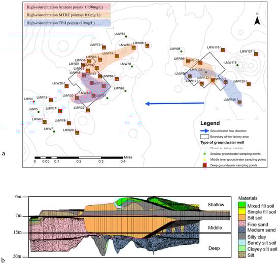
Figure 1. Overview of the study site in the southeast of Beijing. (a) Sampling point distribution map: Shallow sampling wells (green), middle-depth sampling wells (yellow), and deep sampling wells (red). The general direction of groundwater flow is from east to west. (b) Three-dimensional geological structure map of strata. Layered concentrations of benzene, TPH, and MTBE (mg/L).

2.2. Interpolation Tools and Methods

Spatial interpolation methods can transform discrete sampling points into a continuous surface. They are generally divided into two categories: deterministic interpolation and geostatistical interpolation. The former includes methods such as IDW, RBF, GPI and LPI. The latter mainly consists of kriging methods, such as OK, SK, UK and EBK. Deterministic interpolation methods assume that all points are related to each other, and the connection between any two points depends on the distance between them. In contrast, geostatistical interpolation methods use semivariograms to consider the spatial autocorrelation between any two points.

The interpolation was performed using ArcGIS 10.8 (Esri Inc., Redlands, CA, USA), and the Leave-One-Out Cross-Validation (LOOCV) method was employed for validation. LOOCV iteratively removes one data point from the dataset, uses the remaining points to build the interpolation model, predicts the value at the removed point, and compares this prediction to the measured value. This process is repeated for each data point. The aggregated prediction errors provide an unbiased estimate of model performance [18]. Through LOOCV, each point is systematically removed from the interpolation, and the remaining points are used to interpolate and predict its value. The predicted values are then compared with the measured values. These validation sets help to determine which interpolation model is the best choice for the dataset. Considering the relatively uniform yet significantly variable sample distribution, along with site-specific layered hydrogeological conditions, three interpolation methods (IDW, OK, and RBF) were selected and systematically evaluated for their applicability in predicting the spatial distribution of groundwater contaminants across shallow, medium, and deep layers, using Leave-One-Out Cross-Validation (LOOCV) and metrics including RMSE, R², and Spearman’s correlation coefficient.

2.2.1. IDW

The IDW method assumes that the influence of the prediction point being estimated decreases with increasing distance from its observation points [19]. In other words, the closer the observation point is to the prediction point, the greater the weight assigned to it, and all observation points within the search neighborhood participate in the calculation of the unknown point as of the prediction point.

$${\mathrm{P}}_{\mathrm{i}}={\displaystyle \frac{{\displaystyle {\sum }_{\mathrm{i}=1}^{\mathrm{n}}}{\displaystyle {\mathrm{d}}_{\mathrm{i}}^{-\mathrm{p}}}{\mathrm{o}}_{\mathrm{i}}}{{\displaystyle {\sum }_{\mathrm{i}=1}^{\mathrm{n}}}{\displaystyle {\mathrm{d}}_{\mathrm{i}}^{-\mathrm{p}}}}}$$

(1)

Here, p_i is the predicted value, n is the number of points used for interpolation, d_i is the distance between the prediction point and the observation point, p is the power parameter, and o_i is the observed value.

This method makes no assumptions about the data structure, such as the normality of the data or the variance. The advantage of this method is that it is fast and very suitable for handling large datasets. It should be noted that in cases of local outliers or uneven distribution of sampling points, the IDW method can exhibit a bullseye effect [20].

2.2.2. RBF

RBF is an exact interpolation method that determines weights using basis functions and distances [21]. Conceptually, the RBF method employs basis functions to fit a surface, thereby achieving a minimized surface [22]. The predicted values from RBF can exceed the range of observed values.

$$\mathrm{CRS}: \mathsf{\phi }\left(\mathrm{d}\right)= {\ln (\mathsf{\sigma }\mathrm{d}/2)}^{ 2}+{{\mathrm{E}}_1\left(\mathsf{\sigma }\mathrm{d}\right)}^{ 2}+\mathsf{\gamma }$$

(2)

$$\mathrm{IMQ}: \mathsf{\phi }\left(\mathrm{d}\right)={\displaystyle \frac{1}{\sqrt{{\mathrm{d}}^2+{\mathsf{\sigma }}^2} }}$$

(3)

$$\mathrm{MQ}: \mathsf{\phi }\left(\mathrm{d}\right)=\sqrt{{\mathrm{d}}^2+{\mathsf{\sigma }}^2}$$

(4)

$$\mathrm{TS}: \mathsf{\phi }\left(\mathrm{d}\right)= \ln ({\displaystyle \frac{\mathsf{\sigma }\mathrm{d}}{2}})+{\mathrm{I}}_0\left(\mathsf{\sigma }\mathrm{d}\right)+\mathsf{\gamma }$$

(5)

$$\mathrm{TPS}: \mathsf{\phi }\left(\mathrm{d}\right)={\mathsf{\sigma }}^2{\mathrm{d}}^2\ln \left(\mathrm{cd}\right)$$

(6)

Here, Completely Regularized Spline (CRS) is Completely Regularized Spline, IMQ is Inverse Multiquadric, MQ is Multiquadric, TS is Thin-plate Spline, and TPS is Thin-plate Spline with Tension, d is the distance between the observation point and the prediction point; σ is the smoothing parameter; γ is the Euler’s constant (approximately 0.577216); E₁ is the exponential integral function; and I₀ is the modified Bessel function of the first kind.

The interpolation function constructed using the RBF method is given by:

$$\hat{\mathrm{f}}\left(\mathrm{x}\right) = {\displaystyle {\sum }_{\mathrm{i}=1}^n} {\mathsf{\lambda }}_{\mathrm{i}}\mathsf{\varphi }\left(∥\mathrm{x} - {\mathrm{x}}_{\mathrm{i}}∥\right) + {\displaystyle {\sum }_{\mathrm{j}=1}^m} {\mathrm{c}}_{\mathrm{j}}{\mathrm{p}}_{\mathrm{j}}\left(\mathrm{x}\right)$$

(7)

In this formula x is the coordinate of the point to be interpolated,${ \mathrm{x}}_{\mathrm{i}}$ is the coordinate of the ith known sample point, ϕ is the radial basis function, $∥\mathrm{x} - {\mathrm{x}}_{\mathrm{i}}∥$ represents the Euclidean distance between the two points, λ_i and c_j are undetermined coefficients, obtained by solving a linear system of equations, p_j(x) is a low-order polynomial basis function, n is the total number of known data points, m is the number of polynomial terms.

Given that the pollutant concentrations at the sampling points within the study area are highly variable and generally sparse, and considering that pollutants in groundwater typically exhibit a relatively smooth transition trend, the CRS method was selected for interpolation. This method is particularly suitable for smoothing and can effectively handle noise in the data, especially when the data points are sparse. The CRS method provides strong smoothing effects and can effectively control overfitting, making it appropriate for situations where high smoothness is required.

2.2.3. OK

Kriging methods assume that the spatial variation of environmental variables can be modeled as a random process with spatial autocorrelation [23]. Kriging can minimize the variance of estimation errors without introducing bias, thus providing more accurate interpolation results [24]. There are different types of kriging, including OK, SK, UK, DK, EBK among others. Generally, kriging methods use the experimental semivariogram to describe spatial autocorrelation [25]. The semivariogram (γ(h)) can be described as:

$$\mathsf{\gamma }\left(\mathrm{h}\right) = {\displaystyle \frac{1}{2\mathrm{n}}}{\displaystyle \sum _{\mathrm{i}=1}^{\mathrm{n}}}{\left[\mathrm{Z}\right({\mathrm{x}}_{\mathrm{i}} + \mathrm{h})-\mathrm{Z}({\mathrm{x}}_{\mathrm{i}}\left)\right]}^2$$

(8)

Here, x_i and x_i + h are the observed locations separated by the distance interval h; Z(x_i) and Z(x_i + h) are the observed values of the variable Z at their respective locations; n is the number of observed points.

Kriging methods, similar to IDW, also calculate the weights of surrounding points to estimate the predicted value. However, unlike IDW, kriging methods take into account spatial autocorrelation in addition to distance weighting, using the semivariogram.

Taking OK as an example, the formula for OK is Z(x) = μ + ε(x); where μ is an unknown constant; ε(x) is a random quantity [26]. It can be described by the following formula:

$$\mathrm{z}({\mathrm{x}}_0) ={\displaystyle \sum _{\mathrm{i}=1}^{\mathrm{n}}}{\mathsf{\lambda }}_{\mathrm{i}}\mathrm{z}({\mathrm{x}}_{\mathrm{i}})$$

(9)

Here, z(x₀) is the predicted value at a certain point; λ_i is the weight; and z(x_i) is the observed value.

By combining the previously created semivariogram model, the weights λ_i can be calculated by solving the following system of equations:

$$\left\{\begin{array}{c}{\displaystyle {\displaystyle \sum _{\mathrm{i}=1}^{\mathrm{n}}}}{\mathsf{\lambda }}_{\mathrm{i}}\mathsf{\gamma }({\mathrm{x}}_{\mathrm{i}} - {\mathrm{x}}_{\mathrm{j}}) + \mathsf{\Psi }({\mathrm{x}}_0) = \mathsf{\gamma }({\mathrm{x}}_{\mathrm{j}} - {\mathrm{x}}_0)\\ {\displaystyle {\displaystyle \sum _{\mathrm{i}=1}^{\mathrm{n}}}}{\mathsf{\lambda }}_{\mathrm{i}} =1\end{array}\right.$$

(10)

Here, γ(x_i − x_j) is the semivariance between observation points i and j, γ(x_i − x₀) is the semivariance between observation point i and the prediction point x₀; and λ(x₀) is the Lagrange multiplier introduced to minimize the error variance.

In the interpolation process of this study, the IDW power parameter p was 2; the OK semivariogram model used an exponential model with parameters calculated from the study’s monitoring data; RBF used the CRS (Completely Regularized Spline) basis function, with the smoothing factor σ = 1.2 determined as the optimal value through the Akaike Information Criterion.

2.3. Effectiveness and Accuracy Analytical Method

The effectiveness and accuracy of the three interpolation methods were evaluated using the cross-validation (CV) metrics of Root Mean Square Error (RMSE), mean CV error (Mean CV), coefficient of determination (R²) from polynomial regression, and Spearman’s rank correlation coefficient (rs). RMSE and Mean CV were employed for statistical analysis, while R² and rs were used to evaluate the accuracy of the interpolated results.

RMSE: Measures the magnitude of prediction error, with values closer to zero indicating higher accuracy [27].

$$RMSE =\sqrt{ {\displaystyle \frac{1}{N}}{\displaystyle \sum _{i=1}^n}(Y_i - f(x_i){)}^2}$$

(11)

In the equation, n denotes the total number of observations, ${\mathrm{Y}}_{\mathrm{i}}$ is the measured value at the ith observation point, and $\mathrm{f}({\mathrm{x}}_{\mathrm{i}})$ represents the corresponding model-predicted value.

Mean CV: Indicates systematic bias (smoothing effect). A value > 0 indicates systematic overestimation, <0 indicates underestimation, and ≈0 indicates minimal bias [28].

$$Mean \mathrm{CV} =(1/n){\displaystyle {\sum }_{i=1}^n}(y_i - {\widehat{y}}_i)$$

(12)

In the formula ${\mathrm{y}}_{\mathrm{i}}$ its corresponding model prediction at the ith point, ${\widehat{\mathrm{y}}}_{\mathrm{i}}$ is the measured value.

R²: From the polynomial regression of predicted vs. observed values, indicates the proportion of variance explained by the model. Higher R² indicates better fit [29].

$$R^{2 }=1 - {\displaystyle \frac{{\displaystyle {\sum }_{i=1}^n}({\widehat{y}}_i - y_i{)}^2}{{\displaystyle {\sum }_{i=1}^n}(y_i - {\overline{y}}_i{)}^2}}$$

(13)

In the formula n denotes the total number of observations, ${\widehat{\mathrm{y}}}_{\mathrm{i}}$ is the measured value at the ith point, ${\mathrm{y}}_{\mathrm{i}}$ its corresponding model prediction, and ${\overline{\mathrm{y}}}_{\mathrm{i}}$ the mean of all measured values.

rs: Measures the monotonic relationship (rank correlation) between predicted and observed values, robust to non-normality. Values close to 1 or −1 indicate strong correlation [30].

$$r_s=1 - {\displaystyle \frac{6\sum {\displaystyle d_i^2}}{n(n^2 - 1)}}$$

(14)

In the formula n is the total number of observations and d_i denotes the rank difference between the predicted and observed values at the ith point.

RMSE is used to directly assess the accuracy of interpolation predictions, as RMSE values close to zero indicate that the predicted values are numerically close to the measured values. The mean CV represents the average of the CV errors, which is important for identifying any bias or smoothing effects in the interpolation model [31]. Significant smoothing suggests that the interpolation either overestimates local minima or underestimates local maxima, thereby inaccurately reducing or masking the contrast in concentration variations across the entire site. Thus, if the mean CV is close to zero, there is minimal bias; if the mean CV is above zero, the model systematically overestimates actual values; and if the mean CV is below zero, the model consistently underestimates these values. Additionally, the measured benzene concentrations were compared and plotted against the interpolated predicted benzene concentrations and CV errors [32]. Finally, interpolation maps were created, and the interpolation surfaces were converted from geostatistical analysis layers to rasters using the Geostatistical Analyst Layer to Raster tool.

3. Results

3.1. Pollutant Concentration

Understanding the distribution of pollutant concentrations is crucial for assessing the accuracy of interpolation results and the spatial distribution characteristics (Figure S1a–c, Table S1). the concentrations of the three characteristic pollutants vary significantly and exhibit extreme values at different sampling depths. This is consistent with the properties of TPH and benzene as LNAPLs, which tend to accumulate in the shallow groundwater and migrate to middle and deeper aquifers with fluctuations in the groundwater table. In contrast, due to its high solubility, MTBE becomes enriched primarily in the deeper groundwater.

Further Analysis of Pollutant Concentrations in Each Layer: Results are Presented in Table 1.

Table 1. Descriptive Summary of Total Concentrations of the Three Pollutants.

	Benzene			MTBE			TPH
	Shallow (n = x)	Middle (n = x)	Deep (n = x)	Shallow (n = x)	Middle (n = x)	Deep (n = x)	Shallow (n = x)	Middle (n = x)	Deep (n = x)
Average (mg/L)	7.56	2.64	0.01	0.22	0.22	1.88	11.52	5.24	0.06
Standard Deviation (mg/L)	31.86	9.65	0.02	1.18	1.18	4.68	46.16	20.02	0.06
Variance (mg/L)	1014.90	93.14	0.00	1.38	1.38	21.87	2130.49	400.78	0.00
Min (mg/L)	0.00	0.00	0.00	0.00	0.00	0.00	0.00	0.00	0.00
Max (mg/L)	178.00	52.70	0.11	6.76	6.76	16.10	260.12	111.60	0.30

From the pollutant concentration data, benzene showed the highest average concentration in the shallow layer (7.56 mg/L), significantly decreasing with depth to 0.01 mg/L in the deep layer, while MTBE exhibited relatively similar average concentrations in the shallow and middle layers (both 0.22 mg/L) but increased to 1.88 mg/L in the deep layer. In contrast, TPH demonstrated a clear decreasing trend with depth, with average concentrations of 11.52 mg/L, 5.24 mg/L, and 0.06 mg/L from shallow to deep layers. All contaminants displayed considerable spatial variability, as evidenced by high standard deviations relative to their mean values and large concentration ranges. The original dataset was strongly right-skewed; however, after logarithmic transformation, it conformed to a normal distribution (Shapiro–Wilk test, p > 0.05), thereby meeting the normality assumption required for geostatistical methods such as kriging and supporting subsequent spatial prediction and risk assessment.

3.2. Interpolation Prediction Results

In Benzene interpolation (Figure 2a) all three interpolation methods (DW, RBF, OK) show the core contaminated area (>1.07 mg/L) concentrated within 80–320 m northwest of the study area across shallow, middle, and deep layers. The DW method produces contamination plumes with jagged boundaries; its high-concentration zones (49.5–178 mg/L) appear as discrete points, with isolated patches in the middle layer. The RBF method generates smooth, continuous plumes but overestimates spatial extent, significantly expanding high-concentration areas (13.8–49.5 mg/L), especially forming connected zones in the deep layer. The OK method displays the most natural concentration gradients; its core contamination zone (3.83–12.8 mg/L) extends southeast in an elliptical shape, yet shows localized gaps (<0.001 mg/L) in the shallow layer (Interpolation results are shown in Table S2).

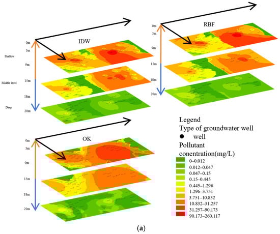
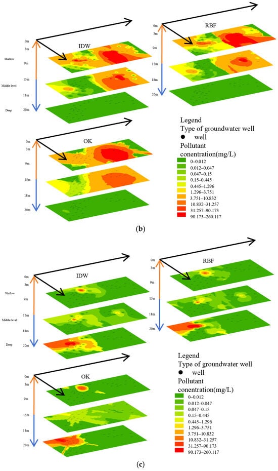
Figure 2. The left side shows the interpolation results for benzene (a), MTBE (b), and TPH (c), while the right side shows the results of polynomial regression analysis.

MTBE interpolation (Figure 2b) all methods identify two core contamination zones in shallow and middle layers: a primary zone east (160–480 m, >31.3 mg/L) and a secondary zone southwest (80 m, >10.8 mg/L). The DWP method forms multi-level ring-shaped concentration bands in the shallow layer; its peak concentration area (90.2–250 mg/L) is smallest with sharp boundaries but shows an anomalous single-point peak (>250 mg/L) in the middle layer. The RBF method creates radially spreading plumes, overestimating low-concentration areas (0.01–0.05 mg/L) east and west while detecting trace contamination (<0.01 mg/L) in the deep layer. The OK method highlights spatial heterogeneity: fragmented patches (1.23–3.71 mg/L) appear west, while the primary eastern zone shows clear concentric stratification (10.8–90.2 mg/L).

As shown in Figure 2c for TPH interpolation, all methods locate the core contamination zone (>0.2 mg/L) within 0–160 m near-field in shallow and middle layers; only RBF detects deep-layer contamination (80 m, >0.3 mg/L). The DW method shows highly localized pollution, with concentrations plunging from 0.4 mg/L at the core to 0.05 mg/L beyond 320 m; no deep-layer contamination is indicated. The RBF method exhibits a shallow-layer “tailing effect” (0.3–0.4 mg/L extending beyond 480 m) and uniquely reveals a deep-layer contamination point; however, non-physical concentration oscillations (0.05/0.2 mg/L alternating bands) occur in the middle layer. The OK method follows distance-decay patterns (smooth 0.4→0.05 mg/L gradient) but underestimates near-field intensity (peak core concentration only 0.3 mg/L); deep-layer data is absent.

3.3. CV Analysis

3.3.1. Statistical Results Analysis

The accuracy of each interpolation method in predicting pollutant concentrations in both space and time was assessed using the RMSE and mean values of the CV obtained during the study period for the IDW, OK, and RBF methods. The RMSE values of the interpolation determined whether the predicted pollutant concentrations matched the measured pollutant concentrations. Values close to zero indicate higher prediction accuracy. Similarly, the mean CV values in the interpolation reflect the smoothing effect and bias. A value greater than 0 indicates an overestimation of concentration, while a value less than 0 indicates an underestimation of concentration. The specific results are shown in Table 2.

Table 2. Cross-Validation Values (Mean CV and RMSE).

Benzene (mg/L)	OK		IDW		RBF
	RMSE	Mean CV	RMSE	Mean CV	RMSE	Mean CV
Shallow	0.03	2.87	0.01	1.98	0.04	1.99
Middle	0.01	0.95	0.09	1.16	0.06	1.45
Deep	0.17	1.56	0.43	1.43	0.16	2.10
MTBE (mg/L)	OK		IDW		RBF
	RMSE	Mean CV	RMSE	Mean CV	RMSE	Mean CV
Shallow	3.55	0.02	2.44	0.01	2.46	4.43
Middle	1.19	0.11	1.45	0.03	1.81	1.49
Deep	1.95	0.54	1.79	0.16	2.63	2.44
TPH (mg/L)	OK		IDW		RBF
	RMSE	Mean CV	RMSE	Mean CV	RMSE	Mean CV
Shallow	0.69	1.06	0.45	1.14	0.15	1.41
Middle	0.28	1.59	1.38	2.14	0.28	2.14
Deep	0.00	1.16	0.01	0.71	0.00	0.91

In the prediction of the concentrations of the three pollutants, the CV values for all methods were greater than 0, indicating that all interpolation methods overestimated the pollutant concentrations. For benzene concentration prediction, IDW had the lowest RMSE in the shallow layers and RBF had the lowest RMSE in the deep layers, indicating the most accurate prediction results, while OK had the lowest RMSE in the middle layer. MTBE, as a petroleum additive, exhibited the same trend as benzene. In the prediction of TPH concentrations, RBF had the lowest RMSE in the shallow layer, and OK had the lowest RMSE in the middle layer, although insignificantly the difference between OK and RBF. In the deep layer, all interpolation methods had relatively low RMSE values, with OK’s RMSE being close to 0. This may be due to the LNAPL nature of TPH, which results in lower pollutant concentrations in the deep layer.

3.3.2. Prediction Error Analysis

The results of the polynomial regression analysis conducted on the concentrations of the three pollutants, the three interpolation methods, and the cross-validation observed and predicted values at different depths are shown in Figure 3.

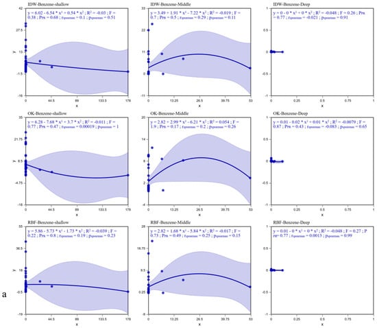
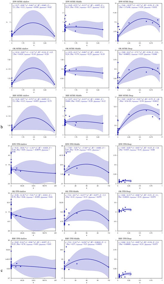
Figure 3. Error Analysis for Benzene (a), MTBE (b), and TPH (c).

For the prediction map, an accurate model displays a regression line with a slope of 1 indicating that the predicted concentration is consistent with the measured concentration. Deviation from a slope of 1 indicates the fitting error of the model. With the increase in depth, the spatial prediction accuracy of pollutants significantly improves, and the reliability of the deep-layer model is much higher than that of the shallow and middle layers (Table 3). Among them, for MTBE in the deep layer, the performance is optimal when using the RBF method (R² = 0.746, F = 47.9, PPR < 0.001). For TPH in the deep layer, the RBF method is also the best (R² = 0.337, F = 9.1, PPR = 0.0008). For benzene, the OK method is preferred in both the shallow and middle layers (shallow layer F = 0.77, middle layer R² = 0.054). Although there is no significant method advantage in the deep layer, the RBF method has relatively better indicators (F = 0.24). Overall, the OK method shows outstanding stability in spatial modeling of pollutants in the shallow and middle layers (for example, TPH in the middle layer has an Spearman correlation of 0.91), while the RBF method has a significantly stronger ability to capture the distribution of deep-layer pollutants (especially water-soluble components such as MTBE). The IDW method performs poorly throughout, negatively confirming that it is not suitable for the spatial heterogeneity characteristics of pollutants in this study. It is recommended to prioritize the use of the RBF method for deep-layer prediction, and the OK method can be used to optimize the shallow and middle layers, while further integrating environmental variables to improve model accuracy (Accuracy verification results are shown in Table S3).

Table 3. Polynomial regression analysis results.

Benzene	Shallow			Middle			Deep
	IDW	OK	RBF	IDW	OK	RBF	IDW	OK	RBF
R2	−0.03	−0.01	−0.04	−0.02	0.05	−0.02	−0.05	−0.04	−0.05
F	0.38	0.77	0.22	0.70	1.91	0.73	0.19	0.34	0.25
PPR	0.68	0.47	0.80	0.50	0.17	0.49	0.83	0.71	0.78
rspeaman	0.03	−0.19	0.08	0.29	0.25	0.27	−0.06	−0.21	−0.10
Pspeaman	0.85	0.23	0.63	0.11	0.16	0.13	0.74	0.25	0.57
TPH	IDW	OK	RBF	IDW	OK	RBF	IDW	OK	RBF
R2	−0.03	−0.01	−0.04	0.00	0.08	0.00	0.15	0.31	0.34
F	0.44	0.78	0.25	0.97	2.33	1.03	3.77	8.05	9.12
PPR	0.65	0.46	0.78	0.39	0.11	0.37	0.03	0.00	0.00
rspeaman	−0.01	−0.04	0.03	0.51	0.91	0.50	0.31	0.31	0.31
Pspeaman	0.96	0.81	0.85	0.00	0.08	0.00	0.08	0.08	0.07
MTBE	IDW	OK	RBF	IDW	OK	RBF	IDW	OK	RBF
R2	−0.05	0.14	0.06	−0.05	−0.05	−0.06	0.54	0.36	0.75
F	0.10	4.45	2.23	0.21	0.24	0.08	19.51	9.83	47.98
PPR	0.90	0.02	0.12	0.81	0.79	0.92	0.00	0.00	0.00
rspeaman	0.15	0.18	0.05	0.17	0.23	0.28	0.38	0.35	0.54
Pspeaman	0.35	0.26	0.73	0.33	0.19	0.12	0.03	0.05	0.00

Overall, the OK method has the best stability in modeling pollutants in the shallow and middle layers (benzene in the shallow layer has an F value of 0.77; TPH in the middle layer has an Spearman correlation of 0.91), making it suitable for scenarios with strong spatial heterogeneity. The RBF method has a significant advantage in deep-layer prediction (MTBE in the deep layer has an R² of 0.75; TPH in the deep layer has a PPR of 0.0008), especially in accurately capturing the spatial autocorrelation structure of water-soluble pollutants (such as MTBE). The IDW method has no significant advantages throughout, with R² and F values often being the lowest (for example, benzene in the deep layer has an R² of −0.05), proving that it is difficult to adapt to the complex distribution of pollutants.

4. Discussion

4.1. Pollutant Distribution Mechanisms and Interpolation Methods Response

The stratified enrichment of composite pollutants is essentially the result of coupling the physical and chemical processes with hydrogeological conditions. According to the hydrogeological conditions in the study area, it is known that the groundwater flow direction is from east to west with the aquifer granularity southward refinement, which leads to pollutant aggregation in the weakly permeable area in the northwestern part of the area (clay accounted for >40% of the total), and this feature needs to be optimized in the interpolation of spatial weights by means of anisotropic parameters. Based on the “hierarchical-driven mechanism,” this study addresses the distribution differences between shallow-/mid-layer LNAPLs (benzene, TPH) and deep-layer highly soluble contaminants (MTBE), integrating the characteristics of each interpolation method (e.g., OK’s quantification of spatial autocorrelation, RBF’s global smoothing effect) to achieve optimal method matching by layer.

In each stratification interpolation, benzene and TPH in the shallow-middle layer, as typical LNAPLs (density < 1 g/cm³), are buoyancy-driven retention at the air pocket- aquifer interface, and their low solubility (benzene 1.8 g/L) and high Log Kow (benzene 2.13) lead to adsorption retention and formation of a non-uniform contamination plume (e.g., CV = 458% for the shallow layer of TPH). The OK method quantifies this spatial autocorrelation through the semivariance function (R² > 0.85 for the goodness of fit of exponential model). Need the subject quantifies this spatial autocorrelation and significantly reduces the prediction variance in areas where sample points are clustered (e.g., LMW96-1 well cluster). The high solubility (48 g/L) and low adsorption of MTBE in the deeper layers encourage it to percolate with groundwater to the top of the chalky aquifer, where it is blocked by a sudden change in permeability coefficient (K = 10⁻⁵ → 10⁻⁷ cm/s) to form a vertical diffusion front. the CRS basis function of the RBF (with the smallest Akaike’s Information Criterion at σ = 1.2) through the global smoothing effect. law (MTBE deep R² = 0.75), but weakens local anomalies (e.g., sudden drop in concentration in LMW84 well).

4.2. Mechanistic Analysis and Comparative Validation of the Performance of Interpolation Methods

The advantages of each interpolation method with hierarchical driving mechanism are shown in Table 4.

Table 4. Advantages of each interpolation method and hierarchical driving mechanism.

Mould	Core Mechanisms	Applicable Scenarios	Limitations
OK	Modeling of spatial structure based on variational functions	Shallow-middle region of high heterogeneity	Sensitive to trend smoothness, underestimates deep dissolution peaks
RBF	Radial basis function global approximation (CRS suppresses overfitting)	Deep smooth transition zone	Generation of “pseudo-oscillations” in shallow sharp gradient zones
IDW	Distance decay weighting (optimal at P = 2)	Uniform sampler outlier environment	Ignoring spatial correlations, the “bull’s-eye effect” is significant

In this study, the RMSE of the OK method for pollutant prediction in shallow to middle layers was lower than that of the IDW method reported by Xie et al. [11] (RMSE for benzene in the middle layer: 0.01 vs. 0.09); the R² of RBF for deep-layer MTBE prediction (0.75) exceeded that of the OK method reported by Rabah et al. [33] in their groundwater pollutant interpolation study in the Gaza Strip (R² = 0.62).

4.3. Uncertainty Analysis

The effects of factors were quantified by analysis of variance decomposition (ANOVA), from the data variability in terms of the spatial coefficient of variation of 606% for deep benzene concentration, the residuals decreased by 72% after logarithmic transformation (Shapiro–Wilk p > 0.05), and from the aspect of the method selection in the prediction of deep layer MTBE, the differences in the methods led to the fluctuation of the RMSE up to 0.74 (IDW = 1.95 to RBF = 1.21), and from the parameter sensitivity aspect, the RMSE of deep layer TPH decreased and then increased (U-shaped curve) when the RBF smoothing factor σ was increased from 0.5 to 1.5, with the optimal σ = 1.0.

Notably, some low R² values (e.g., benzene in shallow layer, R² = −0.01) indicate limited statistical significance, which is attributed to the extreme spatial heterogeneity of LNAPLs (coefficient of variation = 458% for shallow TPH). However, the practical applicability of the OK model is still supported by two aspects: (1) The predicted high-concentration zones are consistent with field observations (e.g., LMW96-1 well cluster); (2) The model reduces prediction variance in sample-clustered areas by 32% compared to IDW, providing reliable guidance for remediation priority zoning.

This research can inform future groundwater management and pollution remediation efforts in two key ways: (1) Long-term monitoring optimization: The model identifies three critical monitoring zones (the northwest high-concentration area, the deep MTBE diffusion front, and the southern site boundary), where monitoring frequency can be increased to semiannual intervals to track contaminant migration; (2) Long-term environmental decision-making: This hierarchical predictive framework can be incorporated into regional soil and groundwater pollution control plans, supporting sustainable land-use transformation of abandoned industrial sites.

5. Conclusions

This study systematically evaluates the effectiveness of GIS interpolation techniques for predicting layered groundwater contamination. Key findings are:

• The study revealed distinct spatial distribution predictions for different contaminants across layers depending on the interpolation method used. IDW produced jagged plume boundaries in both shallow and middle layers, evident in features like the benzene core zone, and demonstrated sensitivity to localized outliers such as a single MTBE peak observed in the middle layer. RBF generated smoothly continuous plumes but tended to overextend high-concentration areas, as seen in the deep layer benzene prediction, and uniquely identified a deep layer TPH contamination point exceeding 0.3 mg/L. In contrast, OK yielded the most natural concentration gradients, exemplified by the elliptical benzene core zone, though it showed a tendency to underestimate peak concentrations near the source, for instance predicting only 0.3 mg/L for a shallow TPH peak.
• CV results indicated significant performance variations between methods. OK demonstrated superior accuracy for interpolating shallow layer benzene and TPH, achieving a middle layer benzene RMSE of 0.005 and a middle layer TPH rs value of 0.91, attributed to its semi-variogram effectively quantifying spatial autocorrelation. Conversely, RBF delivered the highest precision for deep layer MTBE and TPH interpolation, reflected by a deep layer MTBE R² of 0.75 and a deep layer TPH RMSE of 0.002, as its basis function aligns well with the diffusion patterns of highly soluble contaminants. IDW consistently performed the worst across all layers due to the characteristic bull’s-eye effect resulting from its disregard for spatial correlation. Notably, all interpolation methods exhibited a systematic tendency to overestimate concentrations, evidenced by an average cross-validation error greater than zero.
• Analysis of interpolation mechanisms coupled with pollutant characteristics and hydrogeology explained these findings. Contaminants with low density like benzene and TPH tend to accumulate in shallow and middle layers, exhibiting strong spatial heterogeneity well-suited to the spatial structure model inherent in OK. In contrast, highly soluble MTBE forms diffusion fronts in deep layers, a scenario where RBF, with its global smoothing capability, yields optimal results. Hydrogeological constraints, specifically causing pollutant accumulation in the low-permeability northwest zone, necessitate optimization of anisotropic parameters within the OK framework. However, limitations exist: OK’s sensitivity to trend smoothing can lead to underestimation of dissolved peak concentrations in deep layers, while RBF is prone to generating artificial oscillations in shallow areas characterized by steep concentration gradients.
• This study identified limitations concerning sparse sampling points, parameter sensitivity, and the layer-specific applicability of methods. Future research should address these by increasing monitoring well numbers in critical areas, such as deep permeability transition zones and wells exhibiting sharp concentration drops like the LMW84 well. Parameter optimization tailored to each layer is also recommended: for shallow and middle layer data, prioritize OK with tuned anisotropic parameters; for deep layer data using RBF, determine the optimal smoothing factor σ via U-shaped curve testing. Additionally, implementing automated LOOCV scripts within the ArcGIS interpolation process would help dynamically identify the best parameters for each layer.

References

- Wu, S.; Xiang, Z.; Lin, D.; Zhu, L. Multimedia distribution and health risk assessment of typical organic pollutants in a retired industrial park. Front. Environ. Sci. Eng. 2023, 17, 142. [Google Scholar] [CrossRef]
- Sun, S.; Liu, H.; Konar, M.; Fu, G.; Fang, C.; Huang, Z.; Li, G.; Qi, W.; Tang, Q. Urban groundwater supplies facing dual pressures of depletion and contamination in China. Proc. Natl. Acad. Sci. USA 2025, 122, e2412338122. [Google Scholar] [CrossRef]
- Robles, K.P.V.; Monjardin, C.E.F. Assessment and Monitoring of Groundwater Contaminants in Heavily Urbanized Areas: A Review of Methods and Applications for Philippines. Water 2025, 17, 1903. [Google Scholar] [CrossRef]
- Lu, X.; Fan, Y.; Hu, Y.; Zhang, H.; Wei, Y.; Yan, Z. Spatial distribution characteristics and source analysis of shallow groundwater pollution in typical areas of Yangtze River Delta. Sci. Total Environ. 2024, 906, 167369. [Google Scholar] [CrossRef] [PubMed]
- Shi, H.; Wang, S.; Xu, X.; Huang, L.; Gu, Q.; Liu, H. Spatial distribution and risk assessment of heavy metal pollution from enterprises in China. J. Hazard. Mater. 2024, 480, 136147. [Google Scholar] [CrossRef]
- Hou, Y.; Li, Y.; Tao, H.; Cao, H.; Liao, X.; Liu, X. Three-dimensional distribution characteristics of multiple pollutants in the soil at a steelworks mega-site based on multi-source information. J. Hazard. Mater. 2023, 448, 130934. [Google Scholar] [CrossRef]
- Comber, A.; Zeng, W. Spatial interpolation using areal features: A review of methods and opportunities using new forms of data with coded illustrations. Geogr. Compass 2019, 13, e12465. [Google Scholar] [CrossRef]
- Li, J.; Heap, A.D. A review of comparative studies of spatial interpolation methods in environmental sciences: Performance and impact factors. Ecol. Inform. 2011, 6, 228–241. [Google Scholar] [CrossRef]
- Liu, A.; Qu, C.; Zhang, J.; Sun, W.; Shi, C.; Lima, A.; De Vivo, B.; Huang, H.; Palmisano, M.; Guarino, A.; et al. Screening and optimization of interpolation methods for mapping soil-borne polychlorinated biphenyls. Sci. Total. Environ. 2024, 913, 169498. [Google Scholar] [CrossRef]
- Zhang, S.-Q.; Jiang, T.; Li, M.; Zhang, X.; Ren, Y.-Q.; Wei, S.-C.; Sun, L.-D.; Cheng, H.; Li, Y.; Yin, X.-Y.; et al. Exome sequencing identifies MVK mutations in disseminated superficial actinic porokeratosis. Nat. Genet. 2012, 44, 1156–1160. [Google Scholar] [CrossRef]
- Xie, Y.; Chen, T.-B.; Lei, M.; Yang, J.; Guo, Q.-J.; Song, B.; Zhou, X.-Y. Spatial distribution of soil heavy metal pollution estimated by different interpolation methods: Accuracy and uncertainty analysis. Chemosphere 2011, 82, 468–476. [Google Scholar] [CrossRef]
- Yang, Y.; Jia, M. 3D spatial interpolation of soil heavy metals by combining kriging with depth function trend model. J. Hazard. Mater. 2024, 461, 132571. [Google Scholar] [CrossRef]
- Zhao, W.; Ma, J.; Liu, Q.; Dou, L.; Qu, Y.; Shi, H.; Sun, Y.; Chen, H.; Tian, Y.; Wu, F. Accurate Prediction of Soil Heavy Metal Pollution Using an Improved Machine Learning Method: A Case Study in the Pearl River Delta, China. Environ. Sci. Technol. 2023, 57, 17751–17761. [Google Scholar] [CrossRef] [PubMed]
- Goovaerts, P. Geostatistics for Natural Resources Evaluation; Oxford University Press: New York, NY, USA, 1997. [Google Scholar]
- Engeler, I.; Franssen, H.H.; Müller, R.; Stauffer, F. The importance of coupled modelling of variably saturated groundwater flow-heat transport for assessing river–aquifer interactions. J. Hydrol. 2011, 397, 295–305. [Google Scholar] [CrossRef]
- Amin, M.M.; Veith, T.L.; Collick, A.S.; Karsten, H.D.; Buda, A.R. Simulating hydrological and nonpoint source pollution processes in a karst watershed: A variable source area hydrology model evaluation. Agric. Water Manag. 2017, 180, 212–223. [Google Scholar] [CrossRef]
- Wang, L.; Zhou, Y.; Zhou, Z.; Wu, S.; Xia, L.; Zha, Y.; Yang, P. A Spectral Hierarchical Machine Learning for Predicting Arsenic Concentration in Farmland Soil Using Sentinel-2 Imagery. IEEE Trans. Geosci. Remote Sens. 2025, 63, 1–12. [Google Scholar] [CrossRef]
- Pang, Y.; Wang, Y.; Lai, X.; Zhang, S.; Liang, P.; Song, X. Enhanced Kriging leave-one-out cross-validation in improving model estimation and optimization. Comput. Methods Appl. Mech. Eng. 2023, 414, 116194. [Google Scholar] [CrossRef]
- Isaaks, E.H.; Srivastava, R.M. An Introduction to Applied Geostatistics; Oxford University Press: New York, NY, USA, 1989. [Google Scholar]
- Liu, W.; Zhang, H.-R.; Yan, D.-P.; Wang, S.-L. Adaptive Surface Modeling of Soil Properties in Complex Landforms. ISPRS Int. J. Geo-Inf. 2017, 6, 178. [Google Scholar] [CrossRef]
- Aguilar, F.J.; Agüera, F.; Aguilar, M.A.; Carvajal, F. Effects of Terrain morphology, sampling density, and interpolation methods on grid DEM accuracy. Photogramm. Eng. Remote Sens. 2005, 71, 805–816. [Google Scholar] [CrossRef]
- Ding, Q.; Wang, Y.; Zhuang, D. Comparison of the common spatial interpolation methods used to analyze potentially toxic elements surrounding mining regions. J. Environ. Manag. 2018, 212, 23–31. [Google Scholar] [CrossRef]
- Dai, F.; Zhou, Q.; Lv, Z.; Wang, X.; Liu, G. Spatial prediction of soil organic matter content integrating artificial neural network and ordinary kriging in Tibetan Plateau. Ecol. Indic. 2014, 45, 184–194. [Google Scholar] [CrossRef]
- Oliver, M.A.; Webster, R. A tutorial guide to geostatistics: Computing and modelling variograms and kriging. Catena 2014, 113, 56–69. [Google Scholar] [CrossRef]
- Kravchenko, A.; Bullock, D.G. A comparative study of interpolation methods for mapping soil properties. Agron. J. 1999, 91, 393–400. [Google Scholar] [CrossRef]
- Oliver, M.A.; Webster, R. Kriging: A method of interpolation for geographical information systems. Int. J. Geogr. Inf. Sci. 1990, 4, 313–332. [Google Scholar] [CrossRef]
- Armstrong, J.S.; Collopy, F. Error measures for generalizing about forecasting methods: Empirical comparisons. Int. J. Forecast. 1992, 8, 69–80. [Google Scholar] [CrossRef]
- Yates, L.A.; Aandahl, Z.; Richards, S.A.; Brook, B.W. Cross validation for model selection: A review with examples from ecology. Ecol. Monogr. 2023, 93, e1557. [Google Scholar] [CrossRef]
- Ajona, M.; Vasanthi, P.; Vijayan, D. Application of multiple linear and polynomial regression in the sustainable biodegradation process of crude oil. Sustain. Energy Technol. Assess. 2022, 54, 102797. [Google Scholar] [CrossRef]
- De Winter, J.C.F.; Gosling, S.D.; Potter, J. Comparing the Pearson and Spearman correlation coefficients across distributions and sample sizes: A tutorial using simulations and empirical data. Psychol. Methods 2016, 21, 273–290. [Google Scholar] [CrossRef]
- Gnanachandrasamy, G.; Ramkumar, T.; Venkatramanan, S.; Vasudevan, S.; Chung, S.Y.; Bagyaraj, M. Accessing groundwater quality in lower part of Nagapattinam district, Southern India: Using hydrogeochemistry and GIS interpolation techniques. Appl. Water Sci. 2015, 5, 39–55. [Google Scholar] [CrossRef]
- Ouhakki, H.; El Fallah, K.; El Mejdoub, N. Spatiotemporal interpolation of water quality index and nitrates using ArcGIS Pro for surface water quality modeling in the Oum Er-Rabia watershed. Ecol. Eng. Environ. Technol. 2024, 25, 312–323. [Google Scholar] [CrossRef] [PubMed]
- Rabah, F.K.; Ghabaye, S.M.; Salha, A.A. Effect of GIS interpolation techniques on the accuracy of the spatial representation of groundwater monitoring data in Gaza Strip. J. Environ. Sci. Technol. 2011, 4, 579–589. [Google Scholar] [CrossRef]
Disclaimer/Publisher’s Note: The statements, opinions and data contained in all publications are solely those of the individual author(s) and contributor(s) and not of MDPI and/or the editor(s). MDPI and/or the editor(s) disclaim responsibility for any injury to people or property resulting from any ideas, methods, instructions or products referred to in the content. |
© 2026 by the authors. Licensee MDPI, Basel, Switzerland. This article is an open access article distributed under the terms and conditions of the Creative Commons Attribution (CC BY) license.