Artificial Intelligence Agents for Sustainable Production Based on Digital Model-Predictive Control

Abstract

The article presents an approach to synthesizing artificial intelligence agents (AI agents), in particular, control and decision support systems for process operators in various industries. Such a system contains an identifier in the feedback loop that generates digital predictive associative search models of the Just-in-Time Learning (JITL) type. It is demonstrated that the system can simultaneously solve (outside the control loop) two additional tasks: online operator pre-training and mutual adaptation of the operator and the system based on real-world production data. Solving the latter task is crucial for teaching the operator and the system collaborative handling of abnormal situations. AI agents improve control efficiency through self-learning, personalized operator support, and intelligent interface. Stabilization of process variables and minimization of deviations from optimal conditions make it possible to operate process plants close to constraints with sustainable product qualities. Along with higher yield of target product(s), this reduces equipment wear and tear, utilities consumption and associated harmful emissions. This is the key merit of Model Predictive Control (MPC) systems, which justify their application. JITL-type models proposed in the article are more precise than conventional ones used in MPC; therefore, they enable the operation even closer to process constraints. Altogether, this further improves the reliability of production systems and contributes to their sustainable development.

1. Introduction

Recent years have seen the development of production process control systems at various industrial automation levels (such as automated process control systems, operational control systems, warehouse inventory control, production logistics and supply chain management, production resource and sales management) in the form of intelligent agents also known as Artificial Intelligence Agents (AI agents). AI agent is a powerful tool for making effective decisions through data analysis, resource optimization and automation for sustainable development.

AI agents are defined [1,2,3] as systems capable of analyzing incoming information, making decisions, and taking actions to achieve specific goals. Furthermore, AI agents can simultaneously solve multiple multi-stage tasks, control several processes, or interact with various systems to achieve individual or collective goals.

Another difference between AI agents and traditional AI systems is that the former can improve their performance and productivity through continuous self-learning. According to analysts at Gartner [4], the creation of AI agents is one of the new global trends in AI development, and a wide range of solutions are expected to emerge, including the ones for process control in industrial sector.

Against this background, the development of AI agents representing industrial process control or decision support systems, operating based on predictive JITL models, appears relevant. Associative search models [5] have demonstrated high accuracy and efficiency in control systems of processing and power industries [6]. The algorithm for constructing such models is based on training them using an inductive knowledge base: a collection of patterns extracted from analyzed historical and current data [7].

We describe a conceptual approach to synthesizing AI agents which provide decision support to panel operators. It is demonstrated that the proposed AI agents can simultaneously operate as digital twins, solving control optimization problems, and other complex tasks based on predictive digital models, thereby improving overall control efficiency.

AI agents are represented by control systems with an identifier in the feedback loop. They generate control actions based on predictive models of just-in-time learning (JITL) type [8]. Such a predictive JITL-model is created and relevant at a certain time step, then replaced with a new model at the next step, etc.

We consider systems with an identifier of digital models created using associative search algorithms [9,10], which have demonstrated high performance for various objects. Section 2 describes the method for constructing point models in detail.

Control systems based on associative search models demonstrate high efficiency. In a case study, we demonstrate the effectiveness of such control system. This is achieved through the accuracy of predictive models.

At the same time, two additional tasks can be simultaneously addressed outside the control loop (Section 3): online operator pre-training and mutual adaptation of the operator and the system. The latter task is particularly relevant for teaching the operator and the system to collaborate in effective handling of process upsets.

The accuracy of control system dynamics models is also a key condition for the validity and effectiveness of online pre-training systems, which are subsystems of our AI agent in this study.

A detailed study of pre-training systems and mutual adaptation between humans and systems is planned for the near future.

2. Identification Algorithms

We consider identification algorithms which, unlike traditional ones, do not perform online step-by-step model adjustment, but rather build a new digital model at each time step. Such algorithms belong to Just-in-Time Learning (JITL) type [8].

An important advantage of a modern process control system is its ability to predict emergency situations based on historical and current data [9,10]. According to our algorithms, the controller at any given time instant can develop a control action based on the formalized knowledge about the current situation. Here, we mean inductive knowledge, i.e., patterns extracted by means of data mining [7]. This knowledge, relevant for the current moment, should be used for situation model development.

Algorithms of this type presume:

• Acquisition and integration of data from various sources, such as IoT devices, sensors, other control systems, other information systems (maintenance, human resource, etc.);
• Data analysis;
• Knowledge formation and structuring;
• Knowledge formalization.

2.1. Associative Search Method

In AI agents, we propose to use digital models developed on the basis of associative search method. Such models, on the one hand, are developed in accordance with the JITL principle, and on the other hand, they use inductive knowledge of process dynamics and implement the case-based reasoning scheme, as it will be shown below.

Models of objects, in particular, of dynamic processes (e.g., in processing and power industries) developed by means of associative search algorithms use an inductive knowledge base to construct, at each time step, a process model the best one in terms of the RMS criterion.

Models will be formed at each time step by the system identifier based on process history analysis. Thus, inductive knowledge in our case plays the role of precedents. This information allows us to simultaneously train the system and replenish the knowledge base. The model is fully characterized by a set of past and present values of the object’s inputs and the past values of its outputs.

Generally, such models can be obtained using known identification methods. The choice of the associative search method for predictive control applications is determined, first and foremost, by the high accuracy of the identification model for a wide class of objects, including nonlinear and non-stationary ones [8,9]. Moreover, preliminary training (clustering), with permanent retraining in real time, ensures higher computing speed that may be critical for certain industrial applications.

In the associative search algorithm, the identification model is fully described by values of system’s inputs and outputs, which are stored in the process historian. The collection of statistical datasets (feature values) provides a “digital portrait” of plant dynamics. Inductive knowledge processing is reduced to the retrieval (associative search) of knowledge by its fragment. Here, knowledge can be interpreted as an associative relationship between images. As an image, we will use “feature sets”, i.e., components of the input vectors.

For predicting the state of a dynamic process, the method is effective because it: (i) compensates for the insufficiency of a priori information about the object and (ii) allows for poorly formalized input signals and the structure of the control system for this object.

The associative search method develops a linear model of a nonlinear dynamic object at each time step anew using historical datasets called “associations”. In fact, the method is similar to the estimation of a process state or a production situation, carried out by an expert or a decision-maker such as a shift supervisor or panel operator. Based on this person’s knowledge and experience, associations are formed with similar situations stored in his/her memory. To quickly identify “associations”, methods of data clustering are used. In this way, the inductive knowledgebase is formed.

2.2. Associative Search Algorithm

At each time step, an associative search algorithm builds an approximating hypersurface of the space of input vectors and their corresponding outputs. Thus, at each step, a new model is created, and it is linear even for nonlinear objects. This new model replaces the one, built at the previous step. This is the fundamental difference between the associative search model and traditional identification models with adaptive self-adjustment.

To build a virtual model for a certain time instant, points in the multidimensional space of inputs are selected that are close to the current input vector according to the specified criterion (Euclidean, Manhattan distance or other). The corresponding inductive knowledge base is formed at the stage of preliminary training. Then, a system of linear algebraic equations (SLAE) is solved for the unknown coefficients of the model and the predicted output (Figure 1).

The algorithm builds a new model for each moment $t$, and each point of the global nonlinear regression surface is formed as a result of using “local” linear models.

Unlike classical regression models, for each fixed time instant, input vectors that are close to the current one in terms of a certain proximity criterion are selected from the process history (rather than in chronological backward step sequence).

Let n represent the number of vectors from the history (from time instant 1 to $N$) selected using the associative search criterion. At each time interval $\left\{N-1, N\right\}$, a specific set of n vectors is selected, $1\le n\le N$. The criterion for selecting input vectors from the history to construct a virtual model at a given time instant based on the current state of the object can be as follows. We introduce the “Manhattan” distance (norm in ${\mathfrak{R}}^s$) between the points of the S-dimensional input space:

$$d_{N,N-j}={\sum }_{s=1}^S\left|x_{Ns}-x_{N-j,s}\right|, \forall j\in 1,\dots ,N,$$

(1)

where $x_{Ns}$ are the components of the input vector in the current time instant $N$.

From the triangle inequality we have:

$$d_{N,N-j}\le {\sum }_{s=1}^S\left|x_{Ns}\right|+{\sum }_{s=1}^S\left|x_{N-j,s}\right|, \forall j\in 1,\dots ,N.$$

(2)

Let for the current input vector $x_N$:

$${\sum }_{s=1}^S\left|x_{Ns}\right|=d_N$$

(3)

To construct an approximating hypersurface for $x_{N-j}, j=1,\dots ,N$, we select from the input dataset such vectors $x_{N-j}$ that for some given $D_N$, the following condition is satisfied:

$$d_{N, N-j}\le d_N+\sum _{s=1}^S\left|x_{N-j,s}\right|\le D_N, \forall j\in 1,\dots ,N$$

(4)

where $D_N$ can be selected, e.g., from the condition:

$$D_N\ge 2d_N^{max}=\underset{j}{max}\sum _{s=1}^S\left|x_{N-j,s}\right|.$$

(5)

Other metrics, such as the Euclidean distance, can also be selected as criteria. If the selected domain does not contain a sufficient number of inputs to apply the least squares method, i.e., the corresponding SLAE is unsolvable, then the chosen criterion for selecting points in the input space can be relaxed by increasing the threshold $D_N$.

Assuming that the inputs satisfy the Gauss-Markov conditions, the estimates obtained by the least-squares method are consistent, unbiased, and statistically efficient. This procedure thus enables the best possible result within the available information on the dynamic process under study at the current moment. The training results enable real-time modeling with significantly higher performance than the classical least-squares method. Therefore, this associative search procedure may be called a smart least-squares method [10,11]. Since process historians of present-day control systems have significant capacity, the method promises effective results for a wide range of industrial applications.

To improve the performance of the identification algorithm (during both the training phase and the subsequent plant operation), the clustering technique (dynamic classification, automatic data grouping, “unsupervised learning”) from the data mining family is used [11]. As a result, at any given time instant, each point under study in the multidimensional space can be allocated to a group by assigning it a cluster label. Data clustering performed at the system pre-training stage enables high-speed identification and forecasting. In the associative search task, to select input vectors close to the current one from process historian, a cluster label is determined according to the associative selection criterion, and vectors are selected within the corresponding cluster.

The method for control decision support, based on dynamic modeling of the associative search procedure, is described in detail in [9]. The linear dynamic model looks as follows:

$$y_N={\sum }_{i=1}^M{a}_i{y}_{N-i}+{\sum }_{j=1}^N{\sum }_{s=1}^S{b}_{js}{x}_{N-j,s},\hspace{1em}\hspace{1em}\forall j\in 1,\dots ,N,$$

(6)

where $y_N$ is the forecast of the object’s output by the time instant $N$, $x_N$ is the input vector, $M$ is the memory depth for the output, $N$ is the memory depth for the input, $S$ is the dimension of the input vector.

The model built anew at each time step is not a classical regression. To develop it, not all input data are selected from the historian, but only the ones from the inputs selected according to a specified criterion of proximity to the current input vector. The model structure is determined according to the preliminary correlation analysis of the data. As far as the algorithm uses predictive models, its performance is comparable to that of solving a SLAE. The algorithm’s speed can also be increased by using “clustered” linear models (common to all cluster elements) generated during the training phase.

Real-world data storage capacity is typically significant for the method to deliver effective results in a wide range of industrial and business applications. The applications of the authors’ associative search algorithms in oil refining, power industry (smart grids), transportation logistics, and stock trading are described in [10].

3. Associative Model-Based Control Systems as AI Agents

3.1. Models Based on the Associative Search Method

The use of the proposed predictive smart identification models in closed-loop control, as well as in dynamic process forecasting algorithms, is complicated by the correlation of historical and current inputs, outputs and controls in the model:

$$y\left(n+1\right)= \sum _{i=1}^N{a}_{i}y\left(n+1-i\right)+\sum _{j=1}^Q\sum _{i=1}^M{b}_{ij}{x}_j\left(n+1-i\right)+\sum _{i=2}^R{c}_{i}u\left(n+1-i\right)+u\left(n\right).$$

(7)

The upper limits $N,$ $Q,$ $M$, and $R$ characterize the model’s structure. The procedure for forming the structure and selecting variables from the inductive knowledge base for the model is described in [5]. Unlike (6), Formula (7) also reflects the dependence of the system output on control actions at previous time steps. These data along with the values of real process inputs and outputs are entered into the inductive knowledge base of the control system at the training stage. The system’s outputs and controls must meet the following constraints:

$$\left|y\right|\le Y,\hspace{1em}\left|u\right|\le U,\hspace{1em}Y,U>0.$$

(8)

For the control system, we introduce an extended process input vector:

$$\widehat{x}=\left({\widehat{x}}_1,{\widehat{x}}_2\dots {\widehat{x}}_C\right),\hspace{1em}C=MQ+N+R.$$

(9)

This vector consists of the following groups of components:

• Input values $x_j\left(q\right)$, $q\in \left[n+1-M,n\right],j\in \left[1,Q\right]$;
• Control values $u\left(r\right)$, $r\in [n+1-R,n]$;
• Output values $y\left(p\right)$, $p\in [n+1-N,n]$;

i.e.,:

$$\begin{gathered} \left\{{\widehat{x}}_1,{\widehat{x}}_2\dots {\widehat{x}}_{MQ}\right\}=\left\{\begin{array}{c}{x}_1\left(n\right),x_1\left(n-1\right),\dots ,x_1\left(n+1-M\right),x_2\left(n\right),x_2\left(n-1\right), \\ \dots ,x_Q\left(n+1-M\right)\end{array}\right\}; \\ \left\{{\widehat{x}}_{MQ+1},{\widehat{x}}_{MQ+2}\dots {\widehat{x}}_{MQ+R}\right\}=\left\{u\left(n\right),u\left(n-1\right),\dots ,u\left(n+1-R\right)\right\}; \\ \left\{{\widehat{x}}_{MQ+R+1},{\widehat{x}}_{MQ+R+2}\dots {\widehat{x}}_{MQ+R+N}\right\}=\left\{y\left(n\right),y\left(n-1\right),\dots ,u\left(n+1-N\right)\right\} \end{gathered}$$

(10)

In view of these notations, Equation (7) can be represented as:

$$y\left(n+1\right)={\sum }_{i=1}^C{\alpha }_i{\widehat{x}}_i,$$

(11)

where

$$\begin{gathered} \left\{{\mathsf{\alpha }}_1,{\mathsf{\alpha }}_2\dots {\mathsf{\alpha }}_{MQ}\right\}=\left\{b_{ij}\right\},\hspace{1em}i\in \left[1,M\right],\hspace{1em}j\in \left[1,Q\right]; \\ \left\{{\mathsf{\alpha }}_{MQ+1},{\mathsf{\alpha }}_{MQ+2}\dots {\mathsf{\alpha }}_{MQ+R}\right\}=\left\{c_i\right\},\hspace{1em}i\in \left[1,R\right]; \\ \left\{{\mathsf{\alpha }}_{MQ+R+1},{\mathsf{\alpha }}_{MQ+R+2}\dots {\mathsf{\alpha }}_{MQ+R+N}\right\}=\left\{a_i\right\},\hspace{1em}i\in \left[1,N\right]. \end{gathered}$$

(12)

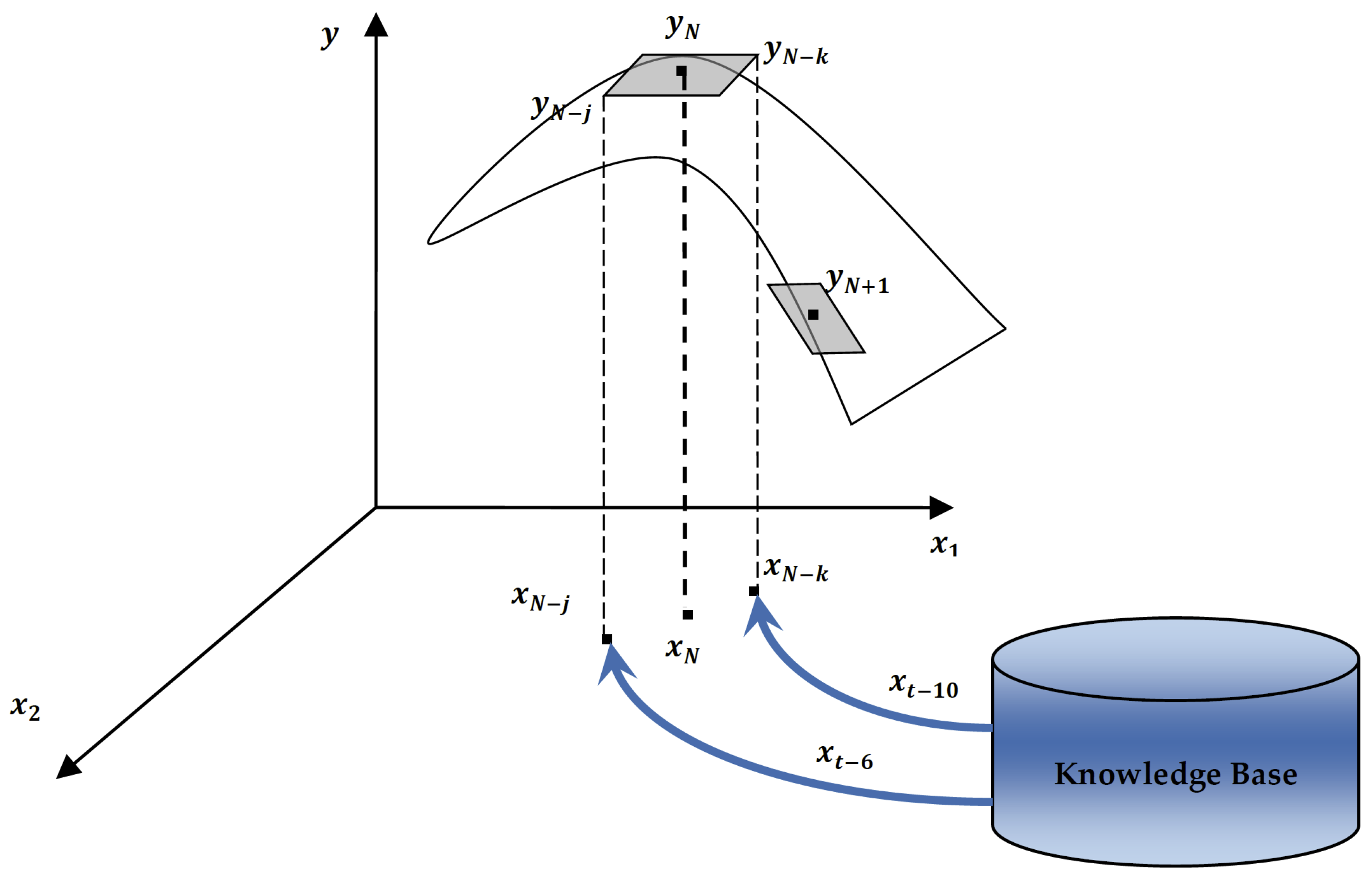
At the first step of the associative search algorithm, the historical data of the extended input vectors are clustered. For developing the model, the algorithm presumes the selection of only those vectors from the cluster which meet a certain criterion of proximity to the current vector ${\widehat{x}}_{search}$, where ${\widehat{x}}_{search}$ is the vector $\widehat{x}$, consisting of input actions and control, i.e.,:

$${\widehat{x}}_{search}=\hspace{1em}\left({\widehat{x}}_1,{\widehat{x}}_2\dots {\widehat{x}}_L\right), L=MQ+R.$$

(13)

As proximity criteria, one can choose, for example, Euclidean or Manhattan distance.

In modern data storage systems, large volumes of data are available for retrieving the required number of extended vectors $P$ to ensure the matrix ${\widehat{X}}^T\widehat{X}$ is well-conditioned. To find the coefficients ${\mathsf{\alpha }}_i$ of the model (11), it is necessary to solve an SLAE of the form:

$$\widehat{X}\mathsf{\alpha }=\widehat{y},$$

(14)

where $\widehat{y}$ is the system’s output at the next step for the selected extended input vectors. In general, the solution to (14) can be expressed as:

$$\mathsf{\alpha }= {\widehat{X}}^{+}\widehat{y}, {\widehat{X}}^{+}={\left({\widehat{X}}^{*}\widehat{X}\right)}^{-1}{\widehat{X}}^{*},$$

(15)

where ${\widehat{X}}^{+}$ is the pseudoinverse matrix for $\widehat{X}$ [12,13].

${\widehat{X}}^{*}$ is the Hermitian conjugate matrix of $\widehat{X}$. Since, in our case, the elements of the matrix $\widehat{X}$ are real, we can replace ${\widehat{X}}^{*}$ with ${\widehat{X}}^{\mathrm{T}}$ in Formula (15).

For relatively large available volumes of historical data, the knowledge base will most probably contain a sufficient number of “input-output-control” sets so that the problem does have solutions. Otherwise (i.e., not enough data), various generative methods can be used in order to form a training sample [14], as well as regularization methods [15,16,17,18,19,20].

Thus, simultaneously with the calculation of the predictive model’s coefficients, the necessary control actions are calculated to be applied at the current time instant. At the same time, the inductive knowledge base is replenished [21], and the system is additionally trained at each step during its operation.

3.2. Digital Twins of Production Processes Based on Identifiers in Feedback Loops

An identifier in feedback loop of a process control system can underlie a new type of digital twins (DT) [22]. In such DT, digital identification models will be used instead of traditional simulation ones.

Traditional DT use simulation models based on first principles modeling (FPM). FPM is a powerful tool for process and control engineering and personnel training [23]. The resulting models accurately reproduce process statics and can simulate their dynamics in various operating modes, but their use for online prediction may become an insoluble problem for the reasons described below.

Simulation models contain dozens of manipulated variables, hundreds of control and disturbance variables (either observable or unobservable), and (often) hundreds of design parameters, which results eventually in high overall dimensionality [24,25,26]. Identifying such models in real time is a computationally intractable task for modern process control systems and is unlikely to be possible within a reasonable timeframe for their development. But even if this were possible for specific process states, the multitude of unmeasured disturbances in a multivariate control object does not guarantee and, as a rule, entirely excludes any sufficiently accurate forecast of the process.

At the same time, the emergence of DT of the identification type, using new methods of predictive object modeling (e.g., in the associative approach), gives FPM a new role. JITL modeling assumes that the space of possible object states is partitioned (clustered) based on the similarity of input-output variable vectors. Doing this from scratch by observing the control object is extremely time-consuming, and using raw historical data requires a complex procedure of initial labeling and contextualizing the identified clusters to define their boundaries. Subsequently, as the plant operates, the set of clusters will be enriched and cluster boundaries may change, but it is convenient to perform the initial labeling at the preliminary synthesis phase using an FPM (once available).

Generally, the synthesis of a control system with an identifier is an ill-posed problem, due to the statistical dependence between the variables in a closed-loop identification algorithm. Control systems with a model adjustable in real time can be synthesized only under appropriate heuristic assumptions. To this end, regularization methods are used.

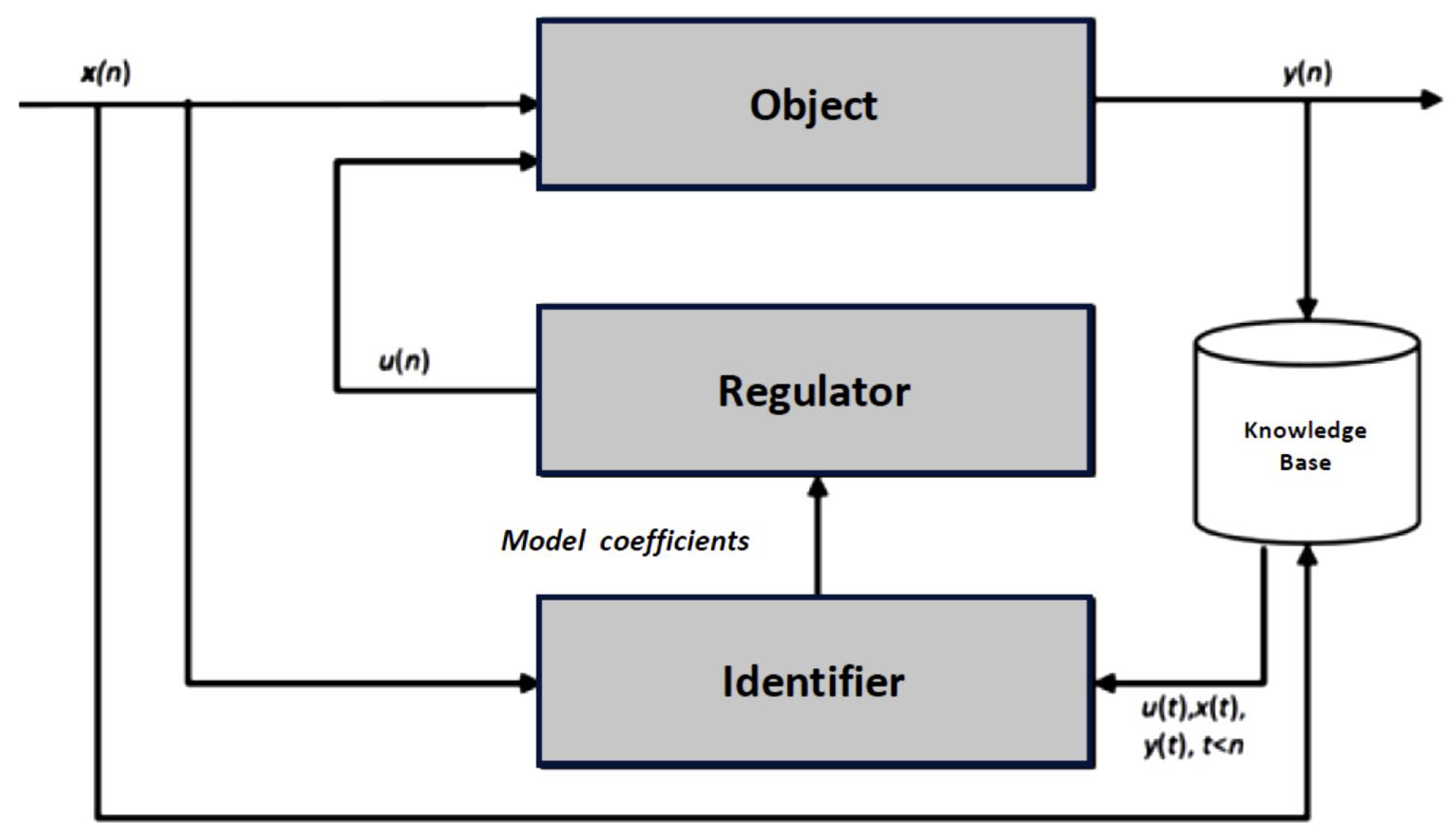
Figure 2 shows a control system diagram in which the identifier in the feedback loop develops a JITL model. The system implements predictive control, and the digital model obtained by the associative search method is its key element.

More data can also be generated using high-fidelity simulation models [23,24].

Identification-type digital twins [22] enable the implementation of associative model predictive control (AMPC) scheme with predictive digital models of the JITL type (see more details in Section 3). The associative models used in this scheme are linear and unique for each time instant. They significantly exceed the accuracy of traditional linearized models. Furthermore, finding the optimal control value does not require solving a linear programming problem each time, as it is required by traditional model predictive control (MPC) technology [24].

3.3. Case Study

Simulation models based on modern physical, stochastic, and empirical approaches can reproduce process nonlinearities and constraints. Modern computing resources allow simulation speeds several times faster than in real time, which makes the simulation system a suitable generator of representative data for identification and controller design [23,24]. This is especially important for processes where long-term field experiments are difficult, risky, or costly.

In this section, we consider a control system with an associative search model identifier, in which process models are pre-trained using high-fidelity simulation ones. The architecture of such a DT [22] includes three key components:

• Inductive knowledge base is an accumulated data set generated through simulation modeling, which includes time series of input, output, and control variables, as well as information on constraints and disturbances. The knowledge base underlies the training of identification models and the subsequent controller design.
• Identifier is a module for generating models based on the analysis of plant history. For predicting plant’s outputs, we will use the identifier for associative models, which were pre-trained using simulation ones with subsequent training on real-world plant data. If the operating mode changes (in which case the associative model may change its structure), additional learning can be conducted using simulation models. Thus, the identifier provides a virtual reproduction of plant dynamics in a digital twin.
• Controller is an algorithm that, using the identifier’s forecast, calculates the optimal control impact taking into account process constraints and the selected control horizon.

The interaction of these components enables the implementation of a closed-loop control system in the DT: at each simulation step, a feature vector is generated, the identifier predicts the system’s response, and the controller develops the corrective action. This approach enables control algorithm testing and debugging in a safe virtual environment before implementing it at the plant. To illustrate the closed-loop control system using a digital twin, we consider ore grinding in a ball mill at a mining and processing plant.

3.3.1. Process Description

Mining and processing plants are complex multi-stage facilities. Each processing stage contributes to the final product quality. Ore grinding is the most energy-intensive stage as well as the most critical one for the efficiency of downstream operations and, eventually, the valuable metal content in the final product. Ball milling features high nonlinearity and complex interrelations between process variables, which makes it especially sensitive to control quality [27,28,29]. A critical aspect here is an accurate representation of the particle size distribution of the ore, because even as small as 5–10% deviation from the optimal size may entail both insufficient grinding quality with resulting metal losses, and excessive grinding, increasing energy consumption by 15–20%.

Stringent quality requirements are driving the development of new identification methods based on data mining and machine learning. Approaches capable of effectively extracting knowledge from diverse historical data look particularly promising. However, accumulating representative historical data is fraught with significant limitations because, for safety and economic reasons, the equipment configured and tuned for continuous optimal operation cannot be stopped on demand or switched to untypical operating modes for acquiring valuable data. It is also prohibited to make abrupt changes in control setpoints as well as exert oscillatory or other functional effects on the grinding process.

Paradoxically, it is data on abnormal situations and boundary conditions that are most valuable for the development of robust control and diagnostic systems. This determines the three-stage strategy for building a process knowledge base. The first stage involves collecting and analyzing data from process historians, which ensures a representative sample of typical operating modes. In the second stage, these data, along with the information from process manuals and equipment datasheets, are used to develop, calibrate, and verify a high-fidelity simulation model that accurately reproduces plant dynamics.

Finally, additional data is generated using the verified model, including particularly valuable scenarios for operating in marginal and abnormal conditions, that are unavailable at the real-life plant. This approach enables the creation of a comprehensive knowledge base that combines the benefits of real plant data and the synthetic data obtained through simulation modeling. Altogether, the approach ensures the necessary completeness and representativeness for the subsequent development of intelligent control systems.

3.3.2. First Principles Modeling of Ball Mill

FPM ensures highly accurate reproduction of the nonlinear and nonstationary dynamics of complex plants such as ball mills. A critical advantage of this approach is the ability to accelerate simulation (up to 100 times faster than real time), ensuring rapid calculations coupled with high fidelity. Simulation models enable safe exploration of both design and abnormal operating modes, including hazardous and emergency situations. This underlies the development of a hybrid knowledge base combining simulated and real-life data.

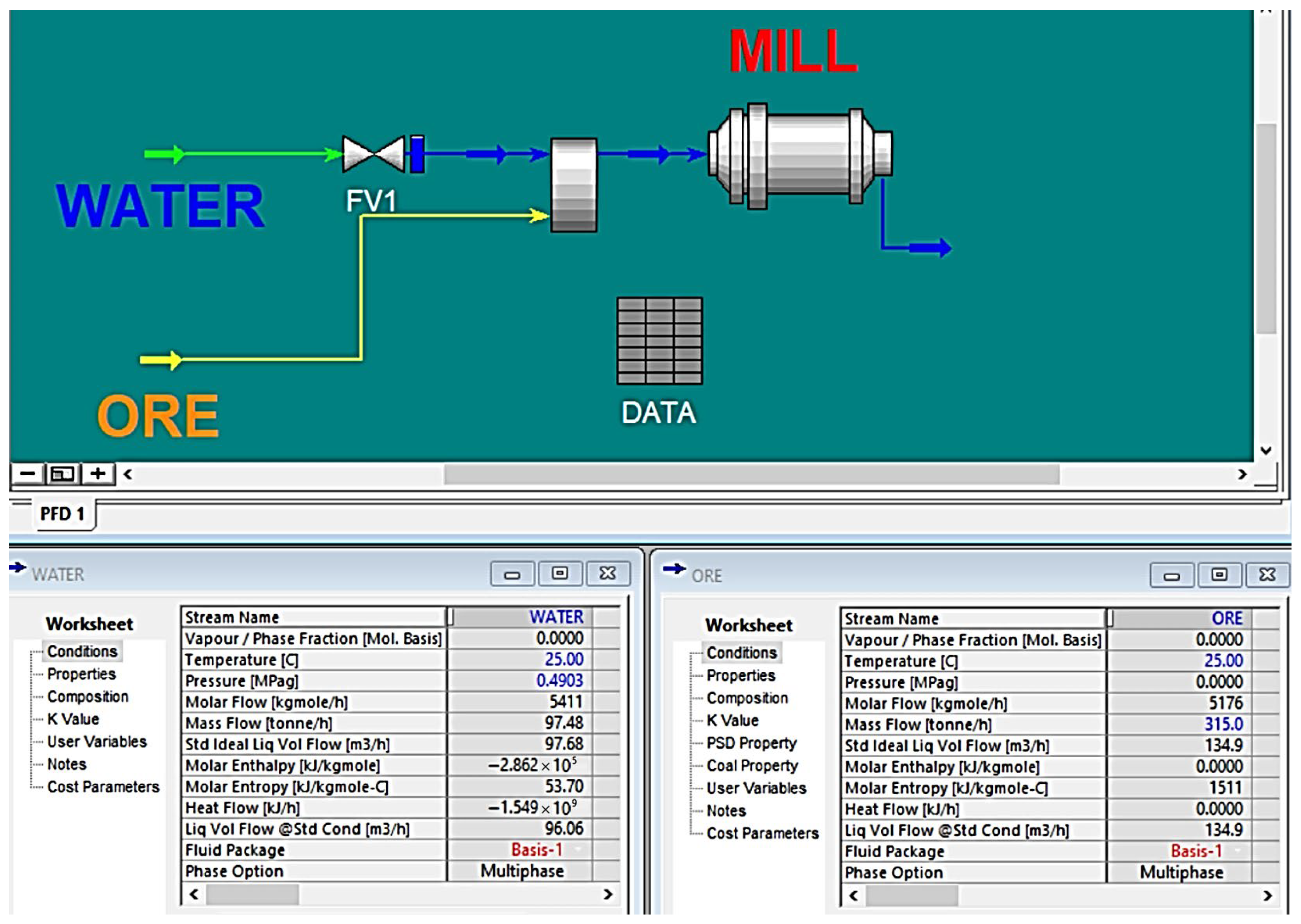
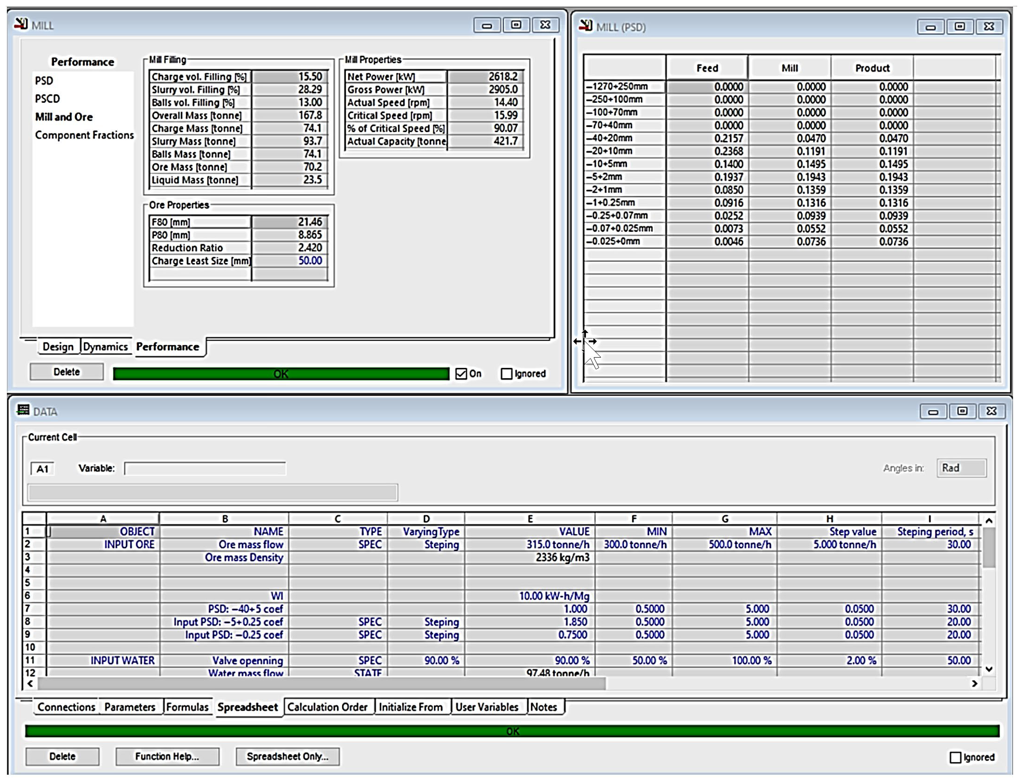
To form a knowledge base, a first principles model was developed. The model allows for material and energy balances, hydrodynamics, grinding kinetics, and other specific features and properties of grinding process and equipment. It employs equipment specifications and operating envelope data from a major Russian mining enterprise.

3.3.3. Ball Mill Operating Principle

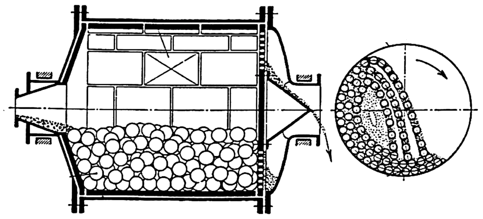
A ball mill is a rotating cylindrical drum (Figure 3) partially filled with grinding media (metal balls). The grinding process occurs through the combined percussive and abrasive action in the cascading motion of the grinding media. As the drum rotates at a certain angular speed, the balls rise along the inner surface of the cylinder to a critical point, whereafter they fall along a parabolic trajectory thus creating intense crushing of ore particles. At the same time, the material is abraded between the balls and the mill lining. Grinding efficiency is determined by the complex interaction of several factors such as:

• Drum rotating speed (60–80% of the critical value);
• Degree of filling with grinding bodies (28–32% of the drum volume);
• The ratio of solid and liquid phases in the slurry;
• Granulometric composition of the ore feed;
• Energy-related parameters of the process.

The ground product is continuously discharged from the mill through a discharge grate (Figure 4). Grinding fineness is controlled by a combination of drum speed, the number and size of grinding bodies, the residence time of the ore in the grinding chamber, and water flowrate. This multifactorial nature and nonlinear relationships between process variables make the ball milling process a complex object to model and control.

3.3.4. Model Variables

The key variables included in the identification model are listed below. They are categorized as follows:

• Manipulated variables (independent variables, control “handles”)

• Ore feed conveyor speed;
• Liquid flow valve opening percentage;
• Mill rotation speed;
• Milling bodies load.

• Disturbance variables (unobservable)

• Mid-grade distribution coefficient;
• Fines distribution coefficient.

• State variables (dependent variables)

• Ore flowrate at mill inlet;
• Water flowrate at mill inlet;
• Water holdup in the mill;
• Slurry volume;
• Crushing ratio;
• Mill rated power.

• Controlled variable (dependent variable, control system’s output)

• Output PSD: −0.25.

The output variable describes the content of particles <0.25 mm in the output ground ore stream. This metric determines the grinding quality and the efficiency of downstream ore dressing operations.

3.3.5. Dataset Detailing and Experimental Methodology

Experimental data were generated using the step-testing technique, in which the manipulated variables were subjected to stepwise changes within acceptable ranges. To ensure the physical feasibility of the generated modes, a comprehensive constraint system was implemented, including: (i) verification of material and energy balances at each modeling step; (ii) monitoring of equipment limitations such as maximum loads and holdup, etc.; (iii) data validation and reconciliation.

The collected data (Figure 5) underwent comprehensive preprocessing. This included diagnostics for outliers and abnormal values, data integrity verification to identify missing and duplicate records, and normalization of all observation vectors to the range [0, 1] to ensure comparability of the scales of various features. The multivariate Pearson correlation analysis was further carried for identifying significant linear relationships between process variables and determining the most informative ones for constructing an identification model.

3.3.6. Identification Model of the Ball Mill Based on Associative Search

The accumulated input data coupled with the corresponding output values provide a knowledge base that can be used for developing various predictive model types. From the variety of approaches to identifying nonlinear dynamic objects, we have chosen the associative search technique.

To process the historical database, as well as implement the associative search algorithm with subsequent analysis of its effectiveness, a software tool was developed in Python 3.10x. and integrated with the simulation model described above.

3.3.7. Results of Preliminary Data Analysis

Pearson correlation analysis identified key relationships between grinding process variables. The most significant correlations include:

• A strong positive correlation between the mill’s rotation speed and its power consumption ($r=0.99$), which confirms the dominant influence of the speed on the power costs;
• Ideal correlation ($r=1.0$) between the volume of slurry in the drum and the accumulated ore mass, indicating a strict relationship between the mill’s loading and filling processes;
• A significant correlation between energy consumption and the grinding ratio ($r=0.83$), which indicates a direct dependence of the quality of crushing on energy costs;
• Negative correlations between the grinding ratio and flow parameters ($r=-0.33\dots -0.3$), indicating a negative impact of mill overload on the grinding quality.

The analysis identified the groups of interdependent variables and filtered out insignificant ones. As a result, an optimal set of historical inputs was formed for the identification model, including values for the mid-grade distribution coefficient at the mill inlet, the fines distribution coefficient, the ore mass flowrate, and the mill speed.

3.3.8. Optimization and Cross-Validation

To determine the optimal number of associations ($k$) in the associative search algorithm, a rigorous optimization procedure was implemented using five-fold cross-validation. The study was conducted with $k$ in the range of [1000; 8000] with a step of 100, which enabled a detailed examination of the dependence of model accuracy on this critical parameter.

Each value of $k$ underwent a full cross-validation cycle: the data was sequentially split into five blocks, with the model trained on four blocks and validated on the remaining one. The approach ensured a statistically reliable assessment of the model’s validation quality, taking into account temporal dependencies in the data.

The optimization results demonstrated a nonlinear dependence of the error on the number of associations, with a clear global minimum at $k=5700$. At this value, the minimum mean square error (MSE) equal to 0.000225 and the maximum coefficient of determination ($R^2$) equal to 0.8634 were achieved.

The analysis showed that decreasing $k$ below the optimal value results in a sharp increase in the error due to insufficient statistical adequacy of local models, while increasing $k$ above the optimal value causes a slight increase in the error due to the inclusion of observations from remote regions of the hypersurface of states.

The selected range of the number of associations essentially represents the sample size required to build a model for a given time instant with high accuracy. Optimizing this value makes it possible to increase the computational efficiency of the algorithm, since the sample size is determined by the algorithm. Its further increase would not improve the accuracy of the estimates significantly.

3.3.9. Comparison to Alternative Methods

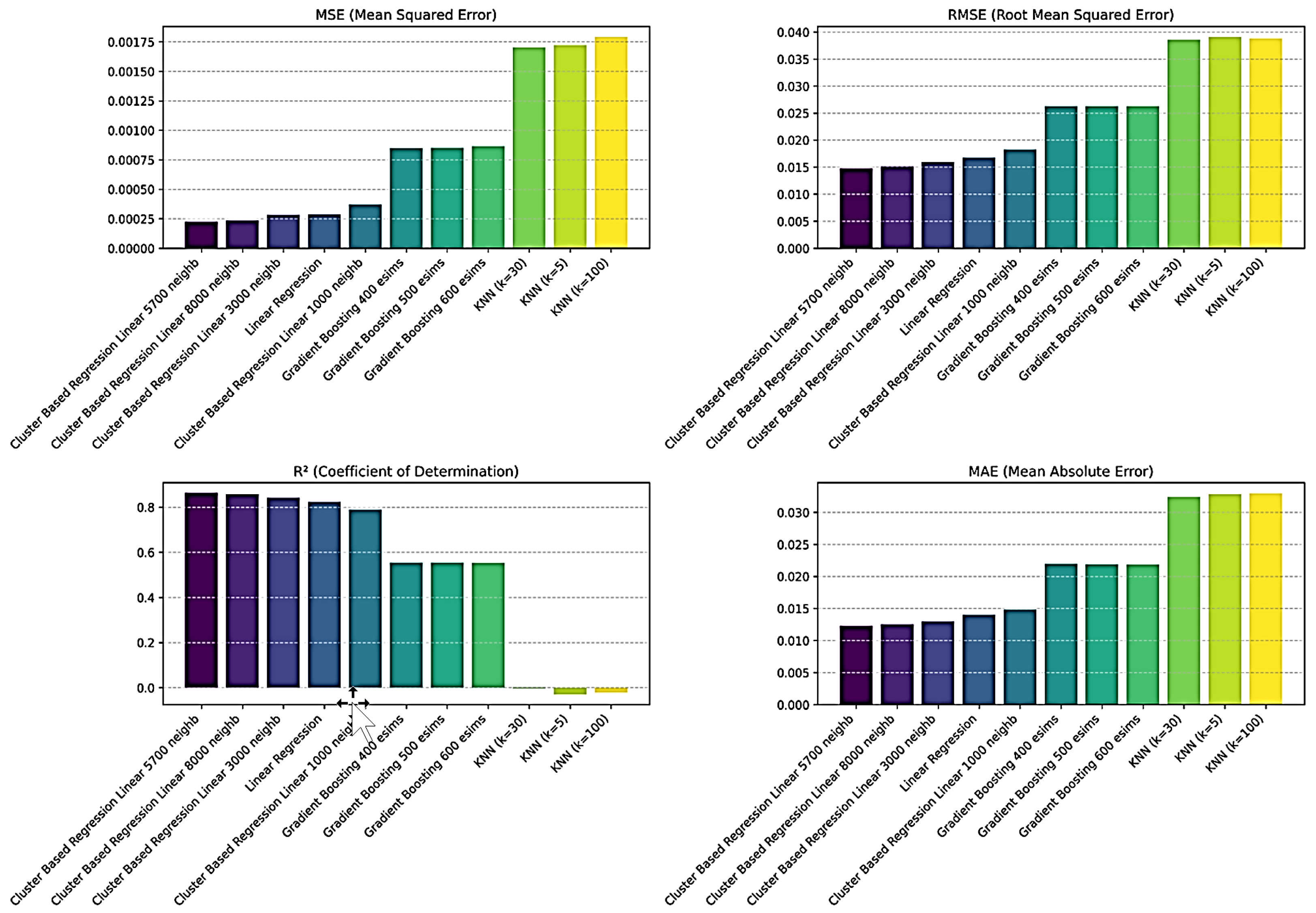
To evaluate the effectiveness of the proposed approach, a comparison was conducted with (Figure 6).; the three alternative identification methods:

• Linear regression
• $k$-nearest neighbors (KNN) algorithm for k = 5; 30; 100;
• Gradient boosting with 400, 500, and 600 estimators.

The comparison was conducted using four key metrics: MSE, RMSE, MAE, and $R^2$. The results, presented in the graphs, convincingly demonstrate the superiority of the associative search model with 5700 “neighbors” (cluster-based regression) across all metrics because it outperforms:

• Linear regression by 78% in MSE (0.000225 vs. 0.00102);
• KNN algorithm for $k=5$ by 42% MSE (0.000225 vs. 0.000385);
• Gradient boosting with 600 estimators by 27% in MSE (0.000225 vs. 0.000308).

The associative search model also demonstrates the highest $R^2=0.8634$, thus confirming its ability to adequately describe the nonlinear dynamics of ball milling. Crucially, the proposed method demonstrates its high accuracy coupled with a significant reduction in computational complexity compared to gradient boosting, that is critical for real-time control systems.

3.3.10. From Identification to Closed-Loop Control

The developed identifier based on associative search is not only a tool for predicting process output parameters but also a fundamental component for building intelligent control systems. High prediction accuracy ($\mathrm{M}\mathrm{S}\mathrm{E}=0.000225, { R}^2=0.8634$) and the model’s ability to adapt to changing operating conditions open up opportunities for synthesizing effective controllers that ensure optimal control of complex nonlinear systems in real time.

The key advantage of the proposed approach is its ability to create a fully digital control loop, where the identification model acts as the plant’s digital twin. Such architecture enables predictive control without building complex analytical models, that is especially relevant for processes with unclear physics or highly nonlinear behavior. It should be noted that traditional control technologies, particularly those using base-level control, often demonstrate insufficient effectiveness when working with objects whose characteristics vary significantly depending on the operating mode. The adaptive approach based on associative search overcomes these limitations by dynamically generating local models that are most relevant to the current state of the object.

Further development of the presented methodology resulted in the creation of an Associative Model Predictive Control (AMPC), which implements a closed-loop control system “Knowledge Base → Identifier → Controller”, providing an end-to-end digital data flow from forecast generation to the calculation of the optimal control impact. This architecture not only inherits the advantages of the developed identifier but also complements them with a mechanism for optimizing control actions, taking into account equipment constraints and process performance targets.

3.3.11. AMPC Operating Principle

At each control step, the algorithm performs the following sequence of operations:

• Based on process history or simulation data, an extended vector of system inputs is generated (see Section 2);
• A search for $k=5700$ closest historical observations in a normalized feature space is performed using the Euclidean distance metric.
• Construction of a local predictive model: based on the identified precedents, a local linear regression model is constructed, which describes the dependence of the output parameter (Output PSD: −0.25) on the input parameters and control impact (mill rotation speed);
• Solving the optimization problem: the optimal control impact $u\left(k\right)$ is calculated, which minimizes the objective function while honoring process constraints.

The key advantage of the AMPC is the development of a new local model at each time step, which is most relevant to the current state of the plant. This allows the controller to effectively compensate for the nonlinearity and non-stationarity of the grinding process.

3.3.12. AMPC Comparison to Base-Level Control

For comparing the AMPC algorithm with an industrial PID controller, a set of synchronized tests was conducted in the simulation environment. The experimental setup included identical first principles models of two ball mills operating in parallel. The first model was controlled by the AMPC algorithm, the second one was controlled by a PID loop tuned by internal model control (IMC) method. Both systems received identical input signals: stepwise changes in the mill speed setpoint (the primary control parameter), as well as synchronized disturbances in ore particle size distribution and water flow. This approach eliminated the influence of external factors and allowed for the evaluation of the net benefits of the control algorithms.

3.3.13. Efficiency Metrics

The controllers were compared across three key groups of indicators. To assess the accuracy of setpoint tracking, integral metrics were used: IAE (Integral Absolute Error), ISE (Integral Squared Error), which handles large deviations, and ITAE (Integral Time-weighted Absolute Error), which penalizes for the duration of transients. Control stability was assessed using the Oscillation Index, Overshoot, and control signal standard deviation (Control_Std), all three directly related with equipment wear risks. Energy efficiency was characterized by the integral squared control (IUE) and the Control Amplitude. All metrics were calculated both over the full-time range of the experiment (suffix_Full) and averaged over setpoint change steps (suffix_StepAvg).

3.3.14. Experiment: Stepwise Change in the Granulometric Composition Setpoint at the Mill Outlet

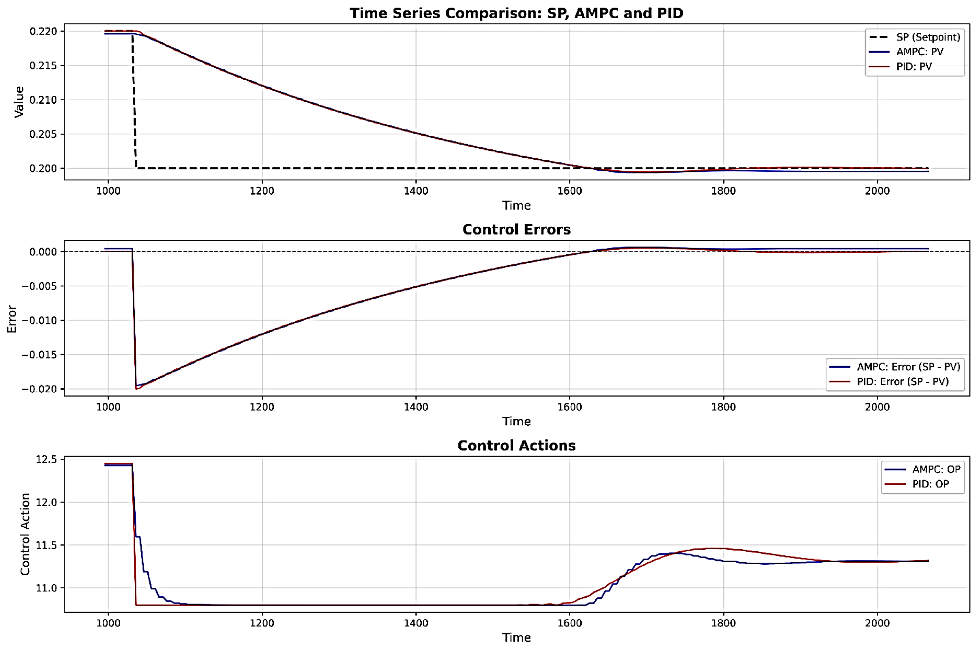
In our scenario, the setpoint for the content of particles smaller than 0.25 mm in the ground product was changed in stages: initially, the value was set at 22%, then decreased to 20%. The total duration of the experiment was 2100 s, which corresponds to the real-life ore grinding process. Both controllers were adjusting mill speed to achieve the target particle size distribution, which enabled the evaluation of their ability to minimize errors when switching between modes with different grinding degrees.

The results showed that the PID loop slightly outperformed the AMPC in terms of setpoint tracking accuracy (see

Table 1. Control Efficiency Metrics (based on the experiment results).

Control Efficiency Metrics	IAE (Integral Absolute Error)	ITAE (Integral Time-Weighted Absolute Error)	Oscillation Index	Control Signal Amplitude (Rotation Speed)	Overshoot, %	Standard Deviation
PID	4.93	6014	1.35	1.651	5.0	0.376
AMPC	5.06	6249	1.00	1.628	4.98	0.364

): the IAE_Full and ITAE_Full values were lower by 2.62% (4.93 vs. 5.06) and 3.76% (6014 vs. 6249), respectively. However, AMPC, implemented based on a regression model demonstrating the dynamics of particle size distribution formation, provided a fundamental advantage in control stability.

The oscillation index for AMPC was 1.00 vs. 1.35 for PID (25.73% lower), and the overshoot decreased to 4.98% (versus 5.0%). This demonstrates the ability of the associative search algorithm to predict the impact of mill speed changes on grinding quality by generating smoother control responses. The approach minimizes the risk of drum load spikes, which occur during aggressive speed adjustments for reaching the setpoint.

The energy efficiency also favored AMPC: the control signal amplitude (rotation speed) decreased by 1.38% (1.628 vs. 1.651), and control variability by 3.27% (StdDev 0.364 vs. 0.376). Against this background, the integrated energy consumption (IUE_Full) remained almost the same (131,237 for AMPC vs. 131,352 for PID). The time to establish the desired particle size distribution for both systems was 207.5 s at each transition stage, confirming AMPC’s operability even with a slow process.

Thus, despite a slight lag in accuracy, AMPC ensured a more moderate operating mode for the equipment thanks to the predictive properties of the associative search model. For ball mills, where abrupt changes in rotation speed accelerate ball and lining wear and tear, this advantage is critical. The obtained results served as the basis for further tests with disturbances emulating real industrial conditions.

The tests revealed the complementary properties of AMPC and PID loops in controlling a ball mill. Under stepwise setpoint changes, AMPC demonstrated advantages in stability and gentle equipment handling, while in scenarios with disturbances, PID showed higher accuracy coupled with increased control aggressiveness.

A key feature of AMPC, based on an associative search model, is its ability to generate smooth control actions, which is critical for slow industrial facilities with high cost of mechanical wear.

AMPC demonstrates the ability to reduce oscillations and control amplitude and compensate for time-dependent inaccuracies under stable disturbances. Further optimization of the model, with the focus on its robustness to granulometric and hydraulic disturbances, will create a solution combining the benefits of predictive control technology with the reliability of proven PID loops (Figure 7).

3.4. Using AI Agents of Production Processes Based on Digital Identifiers of Control Systems for Process Operator Pre-Training

This section describes the possibility of using a digital control system in real-time mode for pre-training process operators. The ability to operate in multitasking mode (along with self-learning capability) is a key property of an AI agent.

With the growing technological complexity, tightening environmental and safety requirements, and the aging of experienced operators in processing industries, the value of computerized training is becoming paramount. An operator training simulator (OTS) is a complex system whose effective utilization depends upon a variety of factors. Trainee’s preliminary awareness of the relationships between process variables is a major key to a successful training session. Developing appropriate concepts during training sessions is typically ineffective, since controlling a complex dynamic object (such as, e.g., a chemical plant), be it a real-world one or its DT, in real time is a dominant mental process that suppresses the learning.

Therefore, various pretraining systems are growing popular. They fill in a methodological gap in operator competence development between theoretical courses and the computerized training. The key objective of such systems is helping the trainee to develop a conceptual model (CM) of the technical system and to form mental skills for controlling it [30,31,32,33,34,35].

In the philosophical tradition, conceptual means existing together with experience, CM is a set of operator’s ideas about equipment pieces, their functions and interrelations, as well as the process as a whole, its current condition, environment, and the ways to control it.

Effective training of emergency responses is possible only when a CM is already established. During special pre-training exercises, mental operator skills are developed, which speeds up and facilitates subsequent online work. This is extremely important, especially in abnormal and emergency situations, where the operator must act quickly and with confidence. Such pretraining can be considered as implicit “learning to learn” [36,37,38,39].

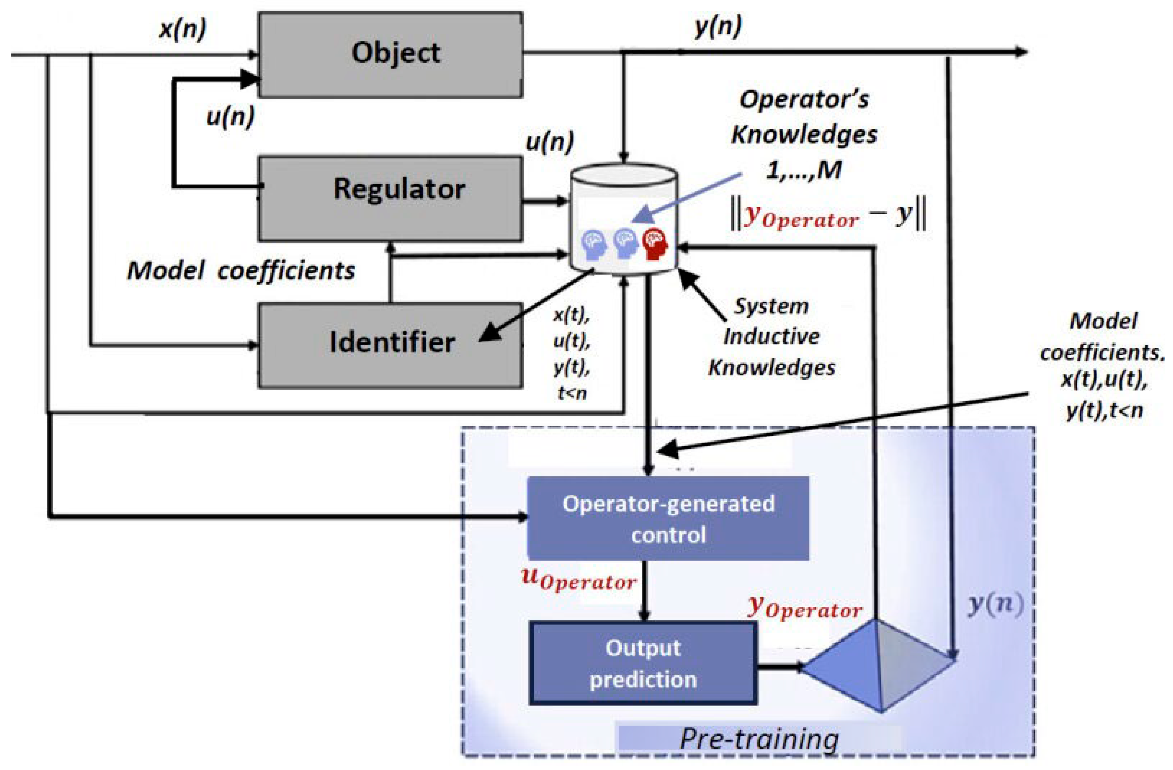
To perform a pretraining procedure, the following scheme can be used (Figure 8), where an AI agent was presented in Section 3.1. For various situations characterized by the state of the process, a certain value of the input vector, and the current content of the inductive knowledge base, the trainee can compare his/her control action generated offline within the “game” to the one calculated by the IA. This can be implemented based on the historical process data (with automatic control or control from other operators). All trainees’ actions in pretraining (not implemented in the real-world control system) are recorded into a dedicated section of the knowledge base (Figure 8). They also represent precedents, and, in turn, can be used for further training of the system.

Thus, analyzing this dedicated section of the knowledge base contributes to stronger mutual adaptation of the operator and the IA.

The use of intelligent agents with the proposed functionality leads to a significant reduction in equipment wear, increased production reliability, prevention of process failures and a reduction in harmful emissions [40,41,42,43].

3.5. Control with IA Adaptation to Operator’s Work Style

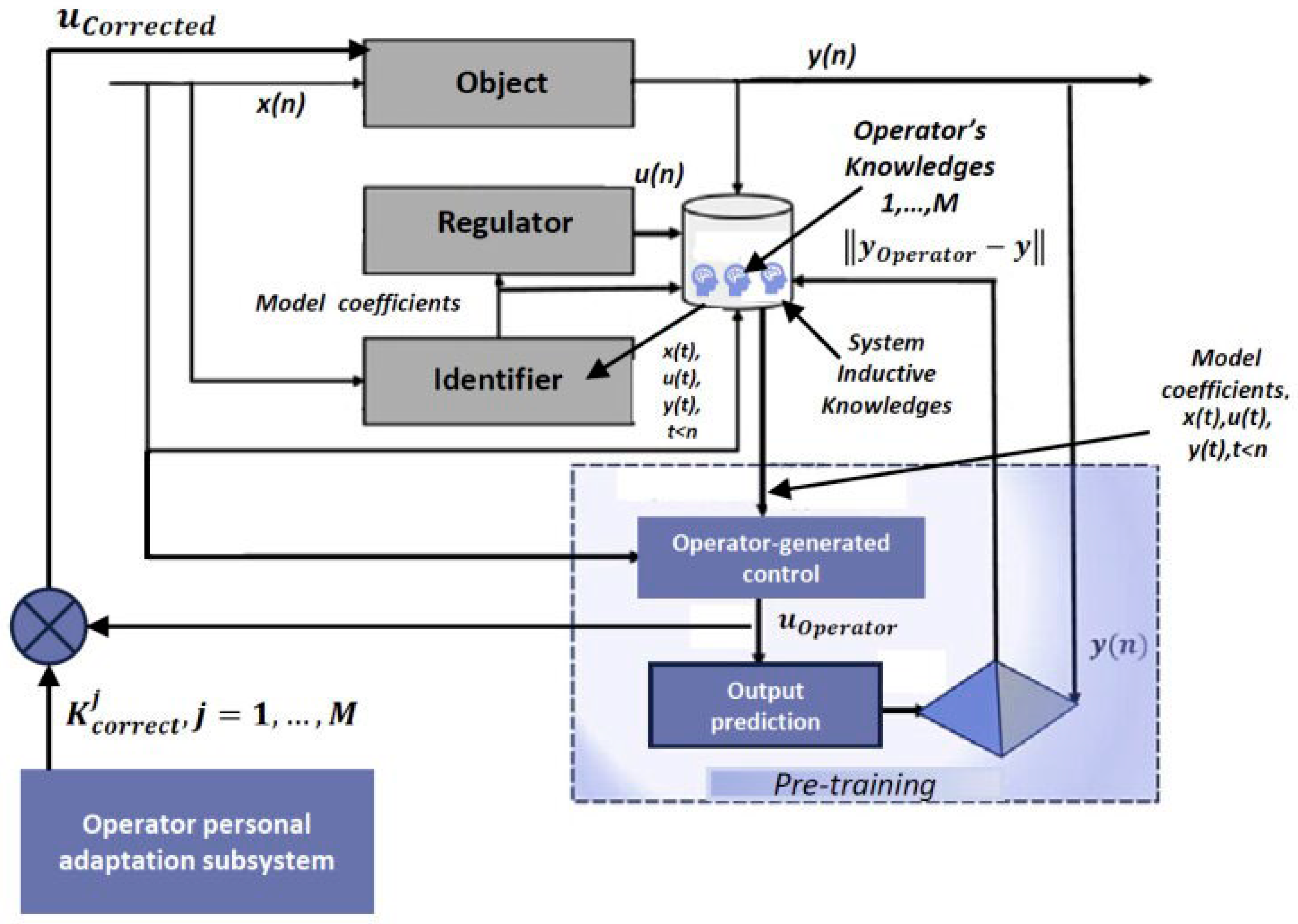
The results of operator pre-training described in the previous subsection are structured and placed in the appropriate modules of the Inductive Knowledge Base. They can be used further in the operation of both a self-learning control system and a subsystem for mutual adaptation of the system and the operator.

The authors are currently studying the possibility of developing a new AI agent type. Specifically, the control action generated in such a system can be further adjusted to suit the operating style of a specific human individual (Figure 9).

The purpose of the Operator/System Mutual Adaptation Module is to improve the efficiency and ergonomics of interaction between the operator and the system. The Module should provide a customized approach with reference to personal, professional, psychophysiological, and behavioral characteristics (such as typical errors and work style) of operators based on continuous analysis of process data. The system generates recommendations to the operator in real time based on the latest results of the analysis.

During the pre-training process, a “portrait of the operator’s activity” is gradually formed in the knowledge base. The appropriate section of the knowledge base is being filled up with:

• Operator response time to changes in process variables;
• Assessment of operator anxiety;
• Control strategies depending on process dynamics;
• Other parameters.

The operator knowledge base should be continuously updated during process control. Based on incoming real-time information, the Module creates a current operator profile based on a combination of indicators (reaction speed, decision effectiveness, unsuccessful decision rate, psychophysiological characteristics, etc.), assesses the operator’s condition, current workload, confidence level, attentiveness, potential fatigue and anxiety, and makes adjustments to recommendations to support decision-making.

The system interface must be able to flexibly change the format of information delivery for specific users in a given situation. Information messages can be presented in the form of textual descriptions, visual images, audio signals, or combinations thereof. The level of screen detail, the range of available functions, the volume and format of prompts, the aggressiveness of alarms, and the information delivery rate must be flexible. For example, an interface with pre-defined scenarios may be more convenient for an unexperienced operator, while an experienced one may benefit from a broader selection of parameters with fewer automated restrictions.

The Module must provide the following functions:

• Individualization of the interface based on a user model (“profile”), determined by personal data, professional experience, current psycho-emotional state, typical errors and the working style.
• Formation of a visual interface in the form of a flexible structure of controlled work processes, where the degree of automation, detailed instructions and contextual help depend on the current tasks and the operator’s skills.
• Implementation of dynamic decision support based on scenario analysis, assessment of critical situations and psychophysiological indicators.
• Monitoring the effectiveness of interface use and actively responding to emerging problems by promptly changing visualization parameters, available functions, and the volume of prompts.
• Reducing errors and increasing process safety by adapting information delivery channels and organizing repetitive procedures.
• Accumulation and recording of scenarios of typical and critical situations, expanded through the accumulation of experience in pre-simulation and simulation training, operation and analysis of the effectiveness of the implementation of interface solutions.
• Allowing for the influence of a set of various factors (for example, let the number of them be equal to $M$, see Figure 9) that characterize the operator’s decision-making style in various situations. In the simplest case, this can be achieved, e.g., by introducing correction factors for all components of the control vector.

As a result, mutual adaptation of human operator and the AI-agent occurs and online pre-training of both the person and the technical system is carried out.

4. Conclusions

The paper has presented an approach to the synthesis of an AI agent as a closed-loop control system with digital predictive JITL models, developed by associative search algorithm. Such a system can operate in multitasking mode, i.e.,: (i) perform the functions of a digital twin, (ii) participate in operator pre-training, (iii) organize the exchange of information between the control system, the inductive knowledge base, the subsystem of personal adaptation of human operator and the subsystem of online pre-training.

Within the proposed AI agent framework, we are planning the development of subsystems for personalized operator adaptation, in particular using scenario forecasting. AI-agent-type control system based on associative forecasting will be able not only to improve control efficiency, but also train the user and provide him/her with personalized support with reference to the current situation. Based on the proposed methodology, AI agents will strive to adaptively increase mutual trust between the control system and the operator, providing personalized support at every step. Research and development of methods for creating intelligent interfaces for AI agents will also be carried out.

So, we have described an approach to creating a class of AI agents capable of simultaneously solving multiple process control tasks while simultaneously self-learning.

AI agents of the type discussed in this paper improve production efficiency through proactive control based on highly accurate intelligent models, operator training using real-time process data, and mutual adaptation between the operator and the system. Predictive models unique for each specific time instant, based on an inductive knowledge, are highly accurate and interpretable. This unique property can be used for scenario modeling of control, that can prevent abnormal and emergency situations.

The features of the proposed approach to the generation of control actions are manifested also in its ability to generate smooth control actions, that is especially important for large and inertial industrial plants with high cost of mechanical wear. Further improvements in model accuracy with the focus on robustness will enable a solution that combines the merits of predictive control with the robustness and reliability of industrial PID loops. At the current stage of research, using the AMPC scheme is justified by higher accuracy of digital associative models as against the traditional ones. However, the results of the experimental study showed that a number of performance indicators of closed-loop control also indicate the expediency of further development of the proposed approach (see Section 3.3.14 for comments).

The proposed approach to automatic control stabilizes process variables and minimizes their deviations from optimal conditions. This enables the operation of process plants closer to their constraints, which reduces equipment wear, fuel and electricity consumption. Rational use of energy decreases the environmental impact, since energy accounts for up to 50% of atmospheric emissions. Dynamic setpoint adjustment helps to achieve and maintain the most beneficial operation mode of process plants and improve the overall production reliability, which contributes to sustainable development of production systems.