Abstract
Fuel cell commercial vehicles are widely used in commercial transport for their high efficiency and long range. However, in mixed operating scenarios, their energy economy and fuel cell operational stability cannot be fully balanced. Traditional strategies lack adaptability in mixed operating scenarios. Therefore, based on the equivalent factor regulation formula of the Adaptive Equivalent Hydrogen Consumption Minimization Strategy (A-ECMS) and the improved Sparrow Search Algorithm-Long Short-Term Memory (SSA-LSTM) hybrid model, short-term speed prediction and three-stage speed interval division are embedded into the equivalent factor regulation logic. A dynamic equivalent factor regulation strategy integrating SOC deviation is constructed, and an improved Predictive Equivalent Hydrogen Consumption Minimization Strategy (P-ECMS) is finally derived. The SSA-LSTM algorithm is optimized via constrained hyperparameter tuning for short-term speed prediction. A time-decay weighting mechanism enhances recent speed data weight, with weighted results as inputs to boost accuracy. Moving Average Residual Correction (MARC) is used to verify the speed prediction model accuracy and correct residuals. Multi-scenario tests show that the SSA-LSTM model outperforms the Gated Recurrent Unit (GRU) model in prediction accuracy and generalization ability, providing reliable data support for segmented regulation. With battery SOC deviation and the SSA-LSTM-predicted speed trend as core inputs, combined with three-stage speed interval division, A-ECMS’s equivalent factor regulation formula is improved. The model adopts a segmented dynamic regulation logic to integrate dual factors into equivalent factor adjustment, and it reasonably adjusts the energy output ratio of fuel cells and power batteries according to speed intervals and operating condition changes. In scenarios with significant speed fluctuations and frequent operating condition transitions, power shocks are mitigated by the power battery’s peak-shaving and valley-filling function. Simulation results for C-WTVC and NREL2VAIL show that, compared with traditional A-ECMS, the improved P-ECMS has notable energy benefits, with equivalent hydrogen consumption reduced by 3.41% and 5.48%, respectively. The fuel cell’s state is significantly improved, with its high-efficiency share reaching 63%. The output power curve is smoother, start–stop losses are reduced, and the fuel cell’s service life is extended, balancing the energy economy and component durability.
1. Introduction
Driven by the global energy structural transformation and the “dual carbon” goals, the low-carbon upgrading of the transportation sector is imperative. The International Energy Agency (IEA) [1] points out that fuel cell commercial vehicles, leveraging their advantages of a long range and fast refueling, have significant zero-emission potential in the field of long-distance heavy-duty transportation. Their full-life-cycle carbon emissions are 50–80% lower than those of traditional diesel vehicles (the emission reduction effect depends on hydrogen production methods) [2]. With the implementation of relevant durability test methods in China, system durability has become a core assessment indicator. Moreover, hydrogen consumption accounts for a large proportion of the total cost of ownership (TCO), directly affecting operational economy [3]. In addition, fuel cells exhibit the characteristic of dynamic response lag. Through experiments simulating three vehicle-mounted dynamic load modes, Yang et al. [4] found that fuel cells are prone to significant performance oscillations under high-power (voltage ≤ 0.51 V) and rapidly fluctuating load conditions, with a current density drop of 5–8% after repeated cycles. Non-optimal conditions such as low temperatures can amplify the attenuation effect, and the current density can decrease from 0.6 A/cm2 to 0.35 A/cm2 during high-load phases. Long-term operation will exacerbate component wear and tear, thereby affecting the service life of fuel cells. Meanwhile, the SOC stability of power batteries is crucial to the reliability of the entire vehicle, and the design of efficient energy management strategies remains an urgent issue to be addressed in the industry [5].
The energy management strategies for current fuel cell commercial vehicles are mainly categorized into rule-based and optimization-based approaches. Rule-based strategies are widely adopted due to their real-time performance advantages. Among them, the power-following strategy proposed by Pukrushpan et al. [6] reduces fluctuations by having the fuel cell track the average power, but it suffers from poor adaptability to varying operating conditions. Guo et al. [7] noted in their review that while the fuzzy logic-based rule-type energy management strategy can coordinate the power distribution among fuel cells, batteries, and supercapacitors through interval division and preset rules, and has been widely applied due to its clear logic and ease of engineering, it relies on expert experience for rule design. Consequently, its adaptability under complex operating conditions such as frequent start–stop operations and heavy-load climbing still needs further optimization by integrating driving cycle prediction technology. For optimization-based strategies, Du et al. [8] proposed a dynamic programming-based energy management strategy for fuel cell hybrid electric vehicles, which achieves globally optimal power allocation but has high computational complexity and is difficult to apply in real time due to its dependence on prior knowledge of driving cycles. Jia et al. [9], when proposing an adaptive model predictive control-based energy management strategy for fuel cell hybrid electric vehicles, pointed out that the performance of model predictive control (MPC) depends on vehicle speed prediction accuracy, and the equivalent hydrogen consumption increases significantly when the prediction error exceeds the threshold, so adaptive optimization is needed to improve prediction robustness. Piras et al. [10] proposed the Predictive Equivalent Consumption Minimization Strategy (P-ECMS), which integrates vehicle speed prediction and dynamic constraints of fuel cells. It achieves a 1.4–6.1% reduction in hydrogen consumption under realistic driving conditions and effectively mitigates fuel cell degradation by suppressing power fluctuations, providing a feasible path for real-time energy management that balances economy and durability.
Vehicle speed prediction accuracy is the core bottleneck of strategy optimization. Abduljabbar et al. [11] adopted a single-layer LSTM network for spatio-temporal vehicle speed prediction; validated based on real traffic data from Melbourne freeways in Australia, it is shown that the root mean square error (RMSE) of speed prediction under complex operating conditions still has room for optimization. Zhang et al. [12] proposed a short-term traffic flow prediction model that optimizes LSTM with an improved genetic algorithm (IGA); after adaptive optimization of hyperparameters, the prediction RMSE on the California freeway dataset is lower than that of pure LSTM and other models, with the prediction accuracy improved by over 10%, verifying the enhancement effect of the optimization algorithm. Li et al. [13] proposed an optimized LSTM traffic carbon emission prediction model integrating multi-source features such as the vehicle speed and vehicle type proportion; in field tests on an urban road network, it achieved a 25% reduction in mean absolute error and a 30% reduction in root mean square error, providing support for quantitative decision-making in traffic emission reduction. Existing models have limitations: traditional LSTM mostly adopts a single vehicle speed feature as the input, and prediction residuals are not corrected. Prediction deviations are correlated with historical and surrounding road segment deviations; failure to correct them will lead to error accumulation in emergency scenarios, resulting in discrepancies between predicted and actual vehicle speeds and triggering high-frequency and large-amplitude fluctuations in fuel cell output power. The deviation correlation capture and correction method proposed by Kim et al. [14] has been experimentally verified to improve the model accuracy and enhance the performance in high-error scenarios. More critically, such power fluctuations cause irreversible damage to fuel cells: Pahon et al. [15] confirmed that proton exchange membrane fuel cells under high-frequency triangular pulse current conditions simulating such fluctuations have a 37% faster power decay rate than the steady-state group, and the mass transfer resistance increased to 2.1 times that of the steady-state group. Padgett et al. [16] further found that after aging, the electrochemically active surface area of PtCo catalysts with non-porous carbon supports decays by over 35%, directly leading to an approximately 40% decrease in fuel cell peak power, reduced driving range, and a nearly 30% shortening of the service life. These studies clarify the complete logic chain: accumulated prediction errors trigger power fluctuations, which in turn accelerate fuel cell aging, induce a performance degradation of core components, and ultimately shorten the service life. This highlights the key significance of improving the vehicle speed prediction accuracy, which has value for extending the fuel cell service life and ensuring the stable operation of the system.
In response to the energy economy bottleneck of fuel cell commercial vehicles under complex working conditions and the core issue that existing strategies rely on vehicle speed prediction but suffer from insufficient prediction accuracy, this paper proposes an SSA-LSTM-Based Future Speed Trend-Embedded Equivalent Factor-Regulated Modified P-ECMS for Fuel Cell Commercial Vehicles, for the energy management of fuel cell commercial vehicles. Derived from the Adaptive Equivalent Hydrogen Consumption Minimization Strategy (A-ECMS), this strategy systematically addresses the key issues raised above through targeted module design and improvement. The specific design is as follows: a vehicle operation trend prediction module based on Long Short-Term Memory (LSTM) is constructed, which improves the basic performance of the model through hyperparameter optimization and introduces a time-decay weighting mechanism to process historical vehicle speed data, with value for enhancing the input quality of short-term prediction. Combined with Moving Average Residual Correction (MARC), the model accuracy is further verified and improved, to ensure the reliability of 3 s short-term future vehicle speed prediction, providing solid data support for subsequent equivalent factor regulation and making up for the prediction shortcomings of traditional LSTM models in complex and changing traffic flow scenarios. On this basis, the regulation logic of the equivalent factor is optimized to break through the limitation of traditional A-ECMS, which only relies on the state-of-charge (SOC) feedback of the power battery. The future vehicle speed trend output by the above prediction module is embedded into the regulation process to construct a dynamic equivalent factor model integrating SOC deviation and vehicle speed prediction trends, which dynamically adjusts the equivalent factor based on dual inputs. Meanwhile, a limit on the maximum power change rate of the fuel cell is added in the power distribution stage to constrain it within a reasonable range, preventing abnormal power fluctuations, effectively suppressing the frequent start–stops of the fuel cell, and ultimately achieving precise energy allocation while ensuring the economic operation of the vehicle.
2. Parallel-Type Fuel Cell Commercial Vehicle Model
In this study, the focus is on parallel-type fuel cell vehicles equipped with a powertrain consisting of a fuel cell and a power battery, whose energy flow and component interaction logic are illustrated in Figure 1. First, hydrogen released from the hydrogen storage tank undergoes an electrochemical reaction with oxygen in the air within the fuel cell to generate electrical energy. On the one hand, this electrical energy, after being regulated by a DC/DC converter, collaborates with the power battery (which features bidirectional energy interaction—supplementing power during the peak demand and recovering energy during braking) to supply power to the DC/AC inverter, thereby driving the motor and rotating the wheels to achieve a power output. On the other hand, electrical energy must be allocated to the auxiliary equipment of the fuel cell system (such as air compressors and water pumps) to ensure the normal operation of core components like the stack. When the vehicle is in braking mode, the motor switches to the generator mode, converting the mechanical energy of the wheels into electrical energy. This energy is then reversely transmitted to the power battery through the DC/AC inverter and DC/DC converter to complete charging, realizing the recovery of regenerative braking energy. In summary, a complete closed loop of energy transmission is formed between the fuel cell, power battery, auxiliary equipment, and drive motor. This not only meets the vehicle’s power requirements under different operating conditions but also significantly improves the energy utilization efficiency through regenerative braking. The vehicle parameters are listed in Table 1.
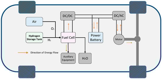
Figure 1.
Structural diagram of parallel-type fuel cell commercial vehicle.

Table 1.
Vehicle parameter table.
Screening of Vehicle Speed Datasets
In this study, the Commercial World Transient Vehicle Cycle (C-WTVC) was selected as the test set, and more than 20 typical domestic and foreign commercial vehicle operating conditions (including WVUCITY, WVUINTER, WVUSUB, NEWYORKBUS, NYCTRUCK, UDDS, JC08, and CHTC series) were simultaneously selected to construct a candidate set. This candidate set fully covers typical driving scenarios, such as urban, suburban, and expressway areas, with its speed distribution and acceleration/deceleration characteristics highly consistent with C-WTVC. It can provide multi-scenario and high-quality data support for the construction of the training and validation sets in this study.
In the field of commercial vehicle operating condition classification, the classical method is a combined paradigm of “multi-feature extraction–Principal Component Analysis (PCA) dimensionality reduction–K-Means Clustering Algorithm (K-Means)” [17]. This method first extracts core kinematic features such as vehicle speed, acceleration/deceleration, and idle speed ratio, simplifies the computational complexity of high-dimensional data through PCA dimensionality reduction, and then realizes the rapid classification of operating conditions via the K-Means algorithm. Although it has the advantage of efficient classification, it has clear defects: it only focuses on the clustering result and lacks the link of quantitative evaluation on the quality of individual data segments, which is prone to a “large quantity but poor quality” of training data and further affects the subsequent model training effect.
To make up for the shortcomings of traditional methods, combined with the driving characteristics of commercial vehicles, this study proposes a combined screening strategy of “rule-based preliminary screening + multi-dimensional fine screening”. Among the stages, the preliminary screening stage aims to quickly define the scenario scope and eliminate clearly abnormal data. It sets clear screening criteria through three key indicators (average speed, idle speed feature, and dynamic constraint) (see Table 2) to rapidly reduce the data scope. As the core link to ensure the data quality, the fine screening stage introduces the quality evaluation framework proposed by Topić et al. [18], constructs a three-dimensional quality evaluation system (including criterion compliance, scenario matching degree, and speed/idle speed rationality), and realizes the quantitative evaluation of the data segment quality through weighted calculation. Meanwhile, it combines Jensen–Shannon (JS) Divergence to quantify the distribution similarity between data segments and C-WTVC, and it sets differentiated thresholds (training set: 0.1~0.2; validation set: 0.2~0.3) to balance the model’s fitting accuracy and generalization ability. For the validation set, the JS Divergence threshold is not set too close to 0, to avoid excessive data overlap, leading to decreased generalization.
Table 2.
Preliminary screening criteria for continuous kinematic segments.
JS Divergence is a symmetric method for measuring the similarity of probability distributions, with a value range of 0~1. The closer the value is to 0, the higher the degree of overlap between the two distributions.
The visualization results of the training set, validation set, and test set are shown in Figure 2. The core function of the validation set is to assist the Sparrow Search Algorithm (SSA) in hyperparameter screening: it screens the optimal and stable hyperparameter combination by quantifying the generalization adaptability of hyperparameters, and it ensures the generalization ability of hyperparameters relying on its preset JS Divergence threshold.
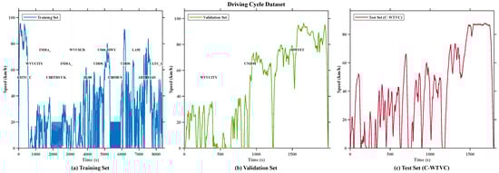
Figure 2.
Training set, validation set, and test set: (a) training set; (b) validation set; (c) test set.
3. SSA-LSTM Vehicle Speed Prediction
3.1. The Process of Optimizing Hyperparameters via the Sparrow Search Algorithm (SSA)
3.1.1. Reasons for Selecting the Sparrow Search Algorithm
LSTM is highly sensitive to hyperparameters in time-series prediction. Traditional empirical parameter tuning or a grid search relies on manual effort and is inefficient, with the computational complexity growing exponentially under high-dimensional parameters. Experiments [19] have confirmed that its feasibility in multi-parameter combination scenarios is extremely low. Vehicle speed prediction is more sensitive to hyperparameters; an improper number of hidden layer units and learning rate can easily lead to underfitting, overfitting, or training oscillations [20]. The Sparrow Search Algorithm (SSA) features fast convergence and a strong global optimization capability. Compared with the Genetic Algorithm (GA), it reduces redundant searches, and compared with Particle Swarm Optimization (PSO), it can avoid local optima [21]. Research on vehicle speed prediction in high-altitude areas [22] proposed that a sample size at the ten-thousand level can effectively support the learning of short-term vehicle speed variation patterns. This paper uses the Sparrow Search Algorithm to optimize the core hyperparameters of LSTM to minimize prediction errors. By considering the empirical ratio of 1:100 between the sample size and the number of hidden units, it fits the short-term temporal characteristics of vehicle speed prediction for the next 3 s, refines the search range of the number of hidden units in LSTM, and thus improves the pertinence and computational efficiency of hyperparameter optimization.
3.1.2. Core Design and Implementation Steps for SSA-Optimized LSTM
In the hyperparameter optimization phase, based on the characteristics of the vehicle speed prediction task, the LSTM hyperparameters to be optimized and their search ranges are determined as follows:
- ➀
- Number of hidden layer units: nunits ∈ [80, 160].
The number of units is the core carrier for LSTMs to capture temporal correlations in vehicle speed. An insufficient number leads to an inadequate model memory capacity, making it difficult to learn long-term dependencies in vehicle speed—for example, the correlation between the current speed and traffic flow status several minutes prior during sustained congestion in peak hours. Conversely, an excessive number causes the model complexity to exceed the supporting capacity of the data, easily leading to overfitting and amplifying noise, such as random fluctuations from accidental acceleration/deceleration or sensor errors. Based on theory and multiple rounds of debugging, the range is ultimately limited to 80–160.
- ➁
- Learning rate α ∈ [0.002, 0.009].
Based on the characteristics of the Adam optimizer, an excessively low learning rate (below 0.002) will result in slow convergence, while a rate exceeding 0.009 will undermine training stability. Hence, this interval is set.
- ➂
- Dropout rate d ∈ [0.12, 0.23].
For small and medium-sized datasets, the dropout rate needs to balance overfitting suppression and feature information retention. Experiments show that 12–23% is the optimal interval.
- ➃
- Sparrow Search Algorithm Optimization Framework with Root Mean Square Error Minimization as the Objective.
The core advantage of the Sparrow Search Algorithm (SSA) lies in achieving efficient optimization by simulating the swarm behavior of sparrows in nature. This study, combined with the task characteristics of vehicle speed prediction, has made corresponding adaptive improvements to the algorithm. The purpose is to obtain hyperparameters that minimize errors such as the root mean square error through optimization, and the required formula is shown in Equation (1) below:
Among the symbols, means taking the parameter vector as the optimization object and minimizing the root mean square error; and are the predicted and actual vehicle speeds, respectively; and is the number of test samples. A 3 s prediction step is selected as the optimization target because this scale exactly matches the look-ahead window for power distribution in the energy management strategy, directly serving the subsequent optimization needs of vehicle energy consumption. The flow chart of the Sparrow Search Algorithm is shown in Figure 3.
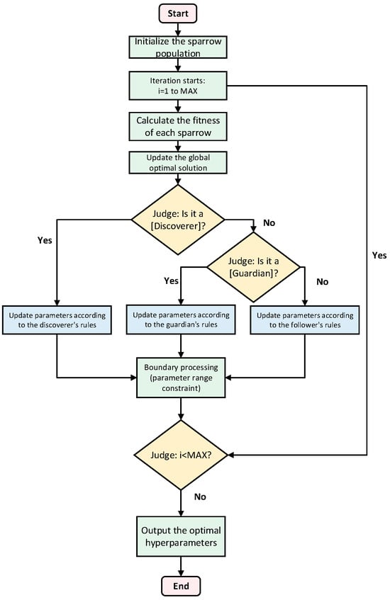
Figure 3.
Flow chart of the Sparrow Search Algorithm (SSA).
3.1.3. Targeted Design of the SSA Optimization Mechanism
- ➀
- Population Initialization.
The core advantage of SSA lies in achieving efficient optimization by simulating the group behavior of sparrows in nature. In this study, corresponding adaptive improvements are made to the algorithm in combination with the characteristics of the vehicle speed prediction task. The initial sparrow position matrix (where N is the population size, and D is the parameter dimension, corresponding to the number of LSTM hyperparameters to be optimized) is generated by the formula shown in Equation (2):
Among them, and are the upper and lower bounds of the preset valid range for the j-th parameter. Subsequently, the generated parameters are verified for physical meaning: the number of hidden layer units is forced to be an integer to avoid meaningless solutions with non-integer units, and the learning rate and dropout rate are truncated at the boundaries to ensure the parameters are within the valid interval. This processing significantly increases the proportion of valid solutions in the initial population compared with the traditional unconstrained random initialization, thereby reducing invalid iterations.
- ➁
- Discoverers (20%).
They are responsible for exploring the search space, and their position update logic is dynamically adjusted according to environmental safety:
When (where ST = 0.8 is the safety threshold), the discoverers explore new regions in an exponential decay manner to expand the search range; otherwise, they perform local fine-tuning for a refined search. This mechanism enables the algorithm to quickly cover the parameter space in the early stage and focus on high-quality regions in the later stage.
- ➂
- Followers (70%).
They improve diversity by imitating discoverers or conducting random searches, and the calculation is as follows:
Among them, and are random numbers following a uniform distribution; t is the current iteration number; represents the global optimal position in the j-th dimension; is the position of the j-th dimension of a randomly selected individual; N is the population size; and i represents the rank of an individual in the population.
- ➃
- Guardians (10%).
They detect and escape local optima, and the calculation is as follows:
is a random number following a uniform distribution, which is used to control the step size of the guardian’s local perturbation. When the individual fitness is better than the global optimum , the randomness of is used to fine-tune the position in the local region, preventing the algorithm from becoming stuck at the current optimal solution and ensuring the completeness of the global search.
To reduce the impact of training on optimization efficiency, a dynamic training strategy is designed: the first three iterations adopt six training rounds for rapid parameter screening, and the subsequent nine iterations increase to eight training rounds to ensure accuracy. Meanwhile, a core step priority optimization strategy is implemented, which only calculates the RMSE of the Nth second prediction step instead of the full-window error. This not only reduces the time consumption of single fitness calculation but also improves the prediction accuracy. Finally, as verified by the validation set, the model achieves an RMSE of 2.98 km/h for the 3 s step on the validation set, effectively verifying that the optimization strategy enhances the prediction accuracy. The hyperparameters optimized based on the Sparrow Search Algorithm are shown in Table 3.
Table 3.
Hyperparameters of LSTM optimized by SSA.
3.2. LSTM Neural Network
There are drawbacks in the indiscriminate processing of traditional historical data: long-term data interferes with prediction, and narrowing the window will lose long-term trends and reduce robustness. Furthermore, the structural design of traditional LSTM makes it difficult to accurately distinguish between long-term trend correlations and short-term instantaneous correlations in vehicle speed data; that is, it lacks pertinence in capturing vehicle speed correlations at different time scales, which will affect its ability to balance long-term trends and short-term fluctuations in vehicle speed prediction tasks. To tackle this, based on the advantage of LSTM in capturing temporal dependencies, this paper sets a 60 s historical window and introduces a time–decay weight mechanism. It assigns differentiated weights to historical information through exponential decay, which not only retains long-term trend information but also enhances the contribution of recent data. Meanwhile, offline residual correction is added after LSTM prediction to calibrate deviations, so as to achieve more accurate short-term vehicle speed prediction.
3.2.1. Composition of LSTM Gating Units
LSTM achieves a selective memory of temporal information through gating units consisting of “forget gate–input gate–output gate”. Each LSTM unit contains gating modules with activation functions and . Through element-wise operations and state transmission, it captures long-term dependency relationships, and the network structure is shown in Figure 4.
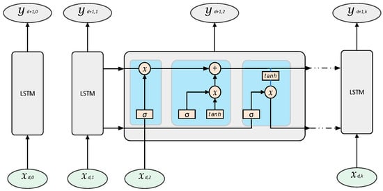
Figure 4.
Structural diagram of LSTM neural network.
3.2.2. Calculation Logic of Each Gating Module
The processing of temporal information by LSTM is accomplished through gating calculations in the following steps:
- ➀
- Forget Gate.
It controls the discarding of historical information and determines which information in the cell state at the previous moment should be forgotten.
where is the Sigmoid activation function (output range [0, 1], quantifying the gating degree); is the hidden layer output at the previous moment; is the current input; is the weight matrix of the forget gate; and is the bias term.
- ➁
- Input Gate.
It regulates the injection of new information and determines which new information in the current input should be incorporated into the cell state.
where is the weight matrix of the input gate; is the bias term; and the definitions of other symbols are the same as those of the forget gate.
- ➂
- Candidate Cell State.
It carries the new temporal features at the current moment and provides candidate content for the update of the cell state.
where denotes the candidate cell state; is the hyperbolic tangent function (normalizing the state value to [−1,1]); is the weight matrix for the candidate cell state; and is the bias term.
- ➃
- Cell State.
It enables the “accumulation and update” of temporal information by integrating the historical cell state (filtered through the forget gate) and the new candidate state (regulated by the input gate).
where ⊙ denotes element-wise multiplication, is the current cell state, and is the cell state at the previous moment.
- ➄
- Output Gate.
It filters the “effective features” for output and determines which information in the cell state should be output to the hidden layer at the current moment.
where is the weight matrix of the output gate, and is the bias term.
- ➅
- Hidden State Output.
It generates the “feature representation” at the current moment, which is the result of the cell state filtered by the output gate and activated by tanh.
The gating mechanism of LSTM endows it with a stronger ability to capture long-term dependencies in time-series prediction tasks. Through the selective forgetting of historical information and selective injection of current information by the forget gate and input gate, the cell state can stably accumulate effective information over a long time series. The output gate further filters key features for the representation at the current moment [23].
3.2.3. Adding a Dropout Layer
- ➀
- Feature Regularization Formula of Dropout Layer.
The Dropout layer is located between the LSTM layer and the layer normalization layer. It receives 90-dimensional abstract temporal features output by the LSTM (integrating both long-term trends and short-term fluctuations of vehicle speed), performs feature regularization through a random masking mechanism, and then passes the processed results to the layer normalization layer, providing a robust input for subsequent optimization of the feature distribution. Its core Formula (12) is as follows:
where h is the feature vector output by LSTM; m is a masking matrix following a Bernoulli distribution (retention rate 1 − p = 0.85, i.e., dropout rate p = 0.15); ⊙ denotes element-wise multiplication; and is used to keep the expected value of features unchanged during the training phase. This layer randomly masks 15% of redundant features to break co-adaptation dependencies between neurons, suppress overfitting, and provide a robust input for subsequent layer normalization, balancing feature utilization and model generalization.
3.3. Time-Decay Weighting Mechanism
- ➀
- Time-Decay Mechanism.
Short-term vehicle speed prediction is primarily influenced by recent speed data, as adjacent-time vehicle speeds exhibit a strong temporal correlation, and this correlation decays exponentially with increasing time intervals. Mozaffari et al. [24] confirmed that reasonable sliding window length optimization is critical for improving prediction accuracy—an overly long window introduces redundant weak-correlation data, while an overly short one loses key temporal dependencies. To match this temporal decay characteristic of vehicle speed data and optimize the weight distribution of historical window input features, this study introduces an exponential time-decay weight mechanism, with the corresponding formula given as follows:
In Formula (13), denotes the original weight at the k-th time step, where k is the index of historical time steps ranging from 0 to L − 1 (L = 60, corresponding to a 60 s historical window). Here, k = 0 corresponds to the current moment, and k = 59 (i.e., L − 1) corresponds to the farthest historical moment. λ is the decay coefficient, determined through multiple experimental trials—we tested various values, including 0.02, 0.05, 0.1, and 0.2, and selected 0.05 as the optimal value based on a comprehensive evaluation of prediction accuracy and the balance between short-term correlation enhancement and long-term trend retention. Within the 60 s window, the cumulative weight of the most recent 10 s accounts for approximately 41.4%, which not only strengthens short-term correlations through the decay characteristic but also retains certain weights for more distant historical data to accommodate long-term trends. In Formula (14), refers to the normalized weight, and represents the sum of original weights across all 60 time steps. Dividing by this sum ensures the total weight equals 1, thus avoiding input scale distortion.
In Formula (15), ⊙ denotes the element-wise product operation, which ensures that vehicle speeds are fused according to their corresponding weights. is the input vehicle speed at the k-th step before time t, and is the finally generated weighted vehicle speed feature, integrating the strongly correlated characteristics of recent vehicle speeds.
The effectiveness of such temporal decay strategies has been widely verified, and their design draws on the core function of the attention mechanism—i.e., focusing on key temporal information by assigning different weights to recent and distant data, ultimately enhancing the contribution of recent data to prediction. For instance, Chughtai et al. [25] implemented dynamic weighting of historical sequences via an attention-based GRU model in short-term travel time prediction, reducing the MAE by 1.64% and RMSE by 0.41% compared with the conventional GRU. The core logic of its weight assignment—prioritizing recent data over distant data—is consistent with the temporal decay strategy proposed in this study. In the field of vehicle emission prediction, He et al. [26] adopted the idea of improving prediction performance through differentiated weighting, and the RMSE of their model was reduced compared with the traditional LSTM. This also indicates that the adoption of a weight assignment mechanism can achieve optimization effects.
3.4. Offline Residual Correction Strategy
To further reduce prediction errors, an offline residual correction module is introduced after the LSTM model is trained. This module only learns residual patterns during the offline phase and does not affect the real-time performance of online prediction. The specific process is as follows:
Residual extraction: Calculate the residuals between the LSTM predicted values and actual values on the training set according to Equation (16):
In Formula (16), ϵ(t) represents the residual, is the actual vehicle speed, and is the predicted vehicle speed.
Residual preprocessing: Median filtering is used to suppress impulse noise while preserving the local trends of residuals, and abnormal residuals outside the interval are corrected (where and are quartiles, and IQR is the interquartile range, i.e., the distance between and ).
Moving average correction: For the prediction results of the test set, a weighted moving average (with a window size of 5 and weights of [0.2, 0.3, 0.4, 0.3, 0.2]) is used to integrate historical residuals for correction:
In Formula (17), is the corrected predicted vehicle speed, is the preprocessed historical residual, and is the weight.
The core of residual correction is to leverage the learnable patterns of model prediction residuals to reduce deviations and minimize RMSE, a logic validated in multiple fields. In the energy sector, Ouyang et al. [27] improved wind power prediction accuracy through residual correction. In the transportation field, Baghoussi et al. [28] proposed a Corrector LSTM with an embedded residual correction module—this model integrates the residual correction structure within LSTM, simultaneously learning the spatio-temporal patterns of residuals during training and inference, ultimately significantly optimizing the RMSE of traffic prediction. This paper adopts the median filtering and moving average method to correct residuals. This method is effective when residuals have strong regularity, but when dealing with noise-dominated irregular residuals, its optimization effect on vehicle speed RMSE is limited. Although residual correction is a post-processing step, it can still assist in road bottleneck assessment and the formulation of traffic diversion plans, reducing congestion and resource waste caused by prediction deviations.
3.5. SSA-LSTM Combined Vehicle Speed Prediction
The traditional Long Short-Term Memory (LSTM) network implicitly captures temporal dependencies through a gating mechanism; however, it encounters significant challenges in small-sample speed prediction tasks. The model’s performance is highly dependent on manual hyperparameter tuning—a time-consuming and suboptimal process that often results in local optima, thereby restricting its generalization capability across diverse operating conditions. Furthermore, the gating mechanism emphasizes feature correlation at the expense of temporal ordering. Despite the higher predictive relevance of recent data, the standard LSTM fails to correlate temporal proximity with predictive importance. This absence of temporal prioritization undermines the model’s responsiveness to abrupt changes in operational dynamics. To address these limitations, this study proposes an enhanced SSA-LSTM model that preserves the inherent temporal modeling strengths of LSTM while incorporating three key improvements. First, a constrained Sparrow Search Algorithm (SSA) is employed for automated hyperparameter optimization, enhancing efficiency and search robustness. Second, a time-decay weighting mechanism is introduced during the preprocessing phase to amplify the influence of more recent vehicle speed observations. Third, a Moving Average Residual Correction (MARC) module is integrated to improve both prediction accuracy and stability. The effectiveness of MARC is directly contingent upon residual characteristics; when residuals exhibit systematic patterns—such as trends or periodicity—the correction effect is pronounced, indicating that underlying structures remain unmodeled and further refinement is warranted. Conversely, if residuals approximate random noise with no discernible pattern, the corrective capacity of MARC diminishes, suggesting that the model has achieved a satisfactory fit and exhibits a strong predictive performance, the specific process of this SSA-LSTM combined vehicle speed prediction is shown in Figure 5.
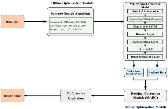
Figure 5.
Flowchart of SSA-LSTM vehicle speed prediction.
The operational workflow of the proposed SSA-LSTM vehicle speed prediction model initiates with data input. The input data are first directed to the Sparrow Search Algorithm (SSA) within the offline optimization module, where key hyperparameters—such as the number of LSTM units, learning rate, and dropout rate—are systematically optimized. The optimized hyperparameters are subsequently transferred to the vehicle speed prediction model. Concurrently, historical data are fed into the model and subjected to time-decay weighting to enhance temporal feature representation. The processed data then sequentially traverse a single-layer LSTM, Dropout layer, normalization layer, fully connected layer with ReLU activation (FC + ReLU), and a de-normalization layer, yielding an initial (uncorrected) vehicle speed prediction and corresponding residual data. These outputs are forwarded to the Moving Average-based Residual Correction module (MARC), in which the residual data are refined using a moving average correction approach to generate corrected vehicle speed predictions.
The corrected predictions then enter the performance evaluation phase, where the root mean square error (RMSE) serves as the core performance metric to assess the residual correction effect: if the RMSE decreases after correction (indicating positive optimization), the corrected vehicle speed data are adopted; if the RMSE increases (indicating negative optimization), the correction result is discarded, and the original uncorrected vehicle speed data are retained. Finally, the result output module delivers a comprehensive report that includes the finalized predicted vehicle speeds and the corresponding error analysis.
Figure 6, respectively, illustrate the comparison between the actual vehicle speed and that predicted by the SSA-LSTM model across prediction horizons of 3 s, 5 s, and 10 s. In the 3 s prediction horizon, the predicted curve exhibits a high degree of conformity with the actual vehicle speed during dynamic scenarios like acceleration and deceleration, accurately capturing short-term speed variation features. This aligns with the conclusion on the LSTM gating mechanism’s strength in filtering historical dynamic information [29]. A slight deviation only occurs in low-dynamic scenarios (e.g., steady or idling speeds) due to sparse feature representation; for the 5s prediction horizon, the predicted curve appears to have a better visual fit, which is actually attributed to the moderate speed fluctuation and reduced complex disturbances inherent in the medium-term prediction context; for the 10s prediction horizon, the deviation between the predicted curve and the actual vehicle speed increases significantly, corroborating the conclusion that prediction error accumulates as the prediction horizon extends [30]. The accuracy exhibits a nonlinear decline as the prediction horizon extends. The core reason lies in long-term road condition uncertainties (e.g., traffic light transitions and abrupt preceding vehicle maneuvers), which impair the model’s capability to characterize dynamic features, ultimately leading to a notable degradation in prediction accuracy.
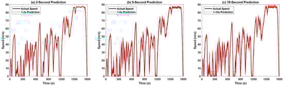
Figure 6.
Vehicle speed prediction results in different time domains: (a) 3 s prediction; (b) 5 s prediction; (c) 10 s prediction.
To determine the optimal time-decay form and corresponding decay coefficient, this study systematically compared and analyzed the prediction performance of four typical functions, namely exponential decay, reciprocal decay, linear decay, and quadratic decay, through multiple sets of control experiments. After multiple parameter adjustments, the relatively optimal coefficient for each function type was selected for subsequent calculations, and their core performance indicators were finally included in the comparison (Table 4). As shown in Table 4, the exponential decay function has the best overall performance at a 3 s prediction step, with a root mean square error (RMSE) improvement rate of 19.65% compared to the no-decay group (Control Group), significantly outperforming the other three decay forms. Therefore, it was adopted as the time-decay feature enhancement scheme in this study.
Table 4.
Comparison table of vehicle speed prediction performance for different decay functions.
In short-term vehicle speed prediction, training data is typically limited, a common small-sample time-series scenario. The LSTM model often struggles to capture the inherent pattern—”recent speed exerts a stronger influence on future values”—due to insufficient data, leading to higher prediction errors. To address that, this study applies feature enhancement via a time-decay mechanism, dynamically weighting a 60 s historical speed window to extract key patterns in advance and reduce model training complexity. Results are presented in Table 5.
Table 5.
Comparison of effects after adopting the temporal decay weight allocation method.
As shown in Table 5, compared with the raw vehicle speed input group, the improved SSA-LSTM with time-decay feature enhancement achieves a notable RMSE reduction of approximately 19.65%, dropping from 3.41 km/h to 2.74 km/h. Even with MARC residual correction, further performance improvement is minimal (only 0.81%), indicating that the enhanced features have effectively captured key driving patterns. This reduces initial prediction errors and thereby limits the corrective potential of MARC. In contrast, the raw vehicle speed group exhibits higher initial errors: the LSTM fails to distinguish the value of different historical data points, leading to incomplete extraction of temporal patterns. The unused regularity retained in the residuals explains why MARC can achieve a 12.62% improvement in this group—highlighting the inadequacy of raw features in small-sample scenarios and the practical utility of time-decay feature enhancement.
The Gated Recurrent Unit (GRU) model serves as the baseline for generalization testing across three operating conditions: Combined World Transient Vehicle Cycle (C-WTVC), National Renewable Energy Laboratory Second Vehicle Activity and Infrastructure Logistics (NREL2VAIL), and New York City Truck Driving Conditions (NYCTRUCK). The root mean square error (RMSE) is adopted as the primary evaluation metric to ensure fairness in the comparison, and the corresponding results are summarized in Table 6.
Table 6.
Generalization test comparison of different models under multiple conditions.
The improved SSA-LSTM outperforms the GRU across all conditions and prediction steps. This advantage comes from the synergy between time-decay feature enhancement (prioritizing recent data, reducing long-term interference) and SSA hyperparameter optimization. The model also shows smaller RMSE fluctuations across conditions, as time-decay-optimized features align with general commercial vehicle driving patterns, paired with SSA’s robust parameters—avoiding the baseline GRU’s poor cross-condition performance.
Test data confirms the algorithm’s effectiveness: across all prediction steps, its performance is markedly improved compared to the non-enhanced group, with limited gains from MARC residual correction—reflecting that the model has fully captured driving patterns. Across multiple conditions, the improved SSA-LSTM outperforms the GRU in both accuracy and generalization.
In summary, the experimental results of multi-condition simulations show that the improved SSA-LSTM algorithm performs feature enhancement on historical vehicle speed data through a time-decay mechanism and uses the enhanced data as the model input. Combined with the precise hyperparameter tuning of the SSA and the efficient capture capability of the LSTM model for temporal dependency relationships, it not only significantly improves the prediction accuracy in the 3–5 s short-term prediction steps but also demonstrates a superior prediction accuracy and generalization stability to the GRU model under various commercial vehicle operating conditions, validating the feasibility of the proposed improvement strategy.
4. Energy Management Strategy Based on Vehicle Speed Prediction
4.1. Prediction-Enhanced A-ECMS
The energy management strategy (EMS) is the core of the powertrain system for fuel cell commercial vehicles, directly determining the vehicle’s hydrogen economy and system synergy efficiency [31]. As reviewed by Khalatbarisoltani et al. [32], the EMS can significantly improve the hydrogen economy and enhance the system synergy efficiency (e.g., extending component lifespan and reducing powertrain fluctuations) by optimizing the power distribution between the fuel cell and energy storage system, with mainstream technical approaches categorized into the Equivalent Consumption Minimization Strategy (ECMS) and its improved variants, as well as Model Predictive Control (MPC). Firstly, the traditional ECMS achieves instantaneous optimization by equating battery charge-discharge energy to hydrogen consumption via a fixed equivalence factor, yet it struggles to adapt to complex dynamic working conditions—a study by He et al. [33] on fuel cell buses confirms that under typical urban dynamic scenarios like start–stop and congestion, the traditional ECMS consumes 6.2% more hydrogen than the Adaptive Equivalent Consumption Minimization Strategy (A-ECMS), directly highlighting the limitations of fixed-factor strategies. Secondly, while A-ECMS balances the real-time performance and optimization effect by dynamically adjusting the equivalence factor based on current states such as SOC, it lags in responding to future working conditions due to its sole reliance on current state feedback. Meanwhile, MPC, grounded in the receding horizon optimization concept, solves the optimal control sequence by predicting system behavior within a finite future time domain, offering a high optimization accuracy but facing a heavy computational burden from complex online solving, which makes it hard to meet the millisecond-level real-time control demands of commercial vehicles.
The traditional Adaptive Equivalent Consumption Minimization Strategy (A-ECMS) relies solely on instantaneous state feedback, unable to predict future operational trends or anticipate subsequent changes in working conditions [34]. This results in suboptimal control decisions and a lag in energy management, ultimately leading to higher hydrogen consumption. To address that issue, this paper proposes an improved Predictive Equivalent Consumption Minimization Strategy (P-ECMS). This strategy retains the core framework of real-time equivalent factor optimization in A-ECMS while incorporating short-term vehicle speed prediction capabilities. By using short-term predicted vehicle speed data to obtain the future short-term operational trend, this trend is then incorporated into the equivalent factor regulation formula to correct the equivalent factor, forming an optimization approach that can not only perceive the current state but also predict future working conditions. This enables decisions to be both responsive and forward-looking. Considering that vehicle speed has a significant impact on power demand and energy consumption, this strategy divides driving scenarios into low-speed, medium-speed, and high-speed intervals. Within each interval, the equivalent factor is adjusted based on changes in short-term predicted vehicle speed, improving the matching degree of energy distribution and subsequent driving conditions. Ultimately, under complex and variable driving conditions, power distribution decisions become more reasonable and adaptable, while also enhancing hydrogen consumption economy and overall system efficiency.
- ➀
- SOC Current Integration Update Formula.
The real-time state of the power battery’s SOC is the basis for strategy decision-making, and its update is based on the current integration model, as shown in Equation (18):
In Equation (18), represents the battery charging/discharging current, and denotes the rated battery capacity. This equation provides real-time feedback on SOC changes, serving as the current state basis for subsequent equivalent factor adjustment. The equivalent factor is the core regulatory parameter for power distribution. The traditional Adaptive Equivalent Consumption Minimization Strategy (A-ECMS) only relies on single-dimensional adjustment of SOC deviation, resulting in a lag in response to dynamic changes in operating conditions.
- ➁
- Static Segmented Equivalent Factor Formula Based on Vehicle Speed Intervals.
The equivalent factor is a core regulatory parameter for power distribution. The traditional Adaptive Equivalent Consumption Minimization Strategy (A-ECMS) only relies on single-dimensional adjustment of state-of-charge (SOC) deviation, resulting in a lag when responding to dynamic changes in operating conditions. In the field of fuel cell vehicle (FCV) energy management, Gao et al. [35] in 2008, for fuel cell buses, divided the intervals of demand power and SOC using fuzzy logic, preset power distribution rules for each interval, and thereby enabled the fuel cell to operate in a high-efficiency region, which effectively reduced the equivalent hydrogen consumption. This rule-based interval regulation strategy, due to its clear logic and ease of engineering, has become a classic early ECMS scheme. By adopting such a method, fixed equivalent factor benchmarks are preset by dividing low-speed, medium-speed, and high-speed intervals to adapt to energy demands at different vehicle speeds and avoid operation in low-efficiency zones. Owing to its clear logic and ease of implementation, it has been widely applied, and based on this, the three-segment formula shown in Equation (19) below is designed:
Here, is a static segmented equivalent factor, while , , and correspond to the segmented values of the equivalent factor in low-, medium-, and high-speed intervals, respectively. By adjusting the coefficient of the initial optimal value of the equivalent factor, differentiated power allocation under different vehicle speeds can be achieved. The initial optimal value of the equivalent factor is derived from the global optimization of dynamic programming. In typical scenarios with gentle operating conditions and no state-of-charge (SOC) constraints, its optimal fixed value is 1.2. Focusing on fuel cell output as the core optimization target, this paper designs three correction coefficients (low, medium, high) for fine-tuning based on to adapt to different vehicle speed requirements.
This strategy exhibits clear static characteristics due to its segmented fixed-value feature: although it can adapt to basic operating conditions through three vehicle speed intervals, it is essentially interval switching of fixed values and cannot achieve continuous dynamic adjustment of the equivalent factor. The core limitation of this segmented step-type regulation is that it struggles to respond to subtle fluctuations in battery SOC and gradual changes in vehicle speed.
Relevant research clearly points out that static segmented strategies lack adaptability to dynamic operating conditions: their fixed-value switching mode tends to cause energy allocation lag under complex operating conditions, which directly leads to a reduced proportion of fuel cell operation in the high-efficiency range, increased efficiency fluctuations, difficulty in maintaining the power battery SOC within the target range, and even the risk of SOC runaway [36].
Therefore, there is an urgent need to introduce a dynamic adaptive mechanism for improvement.
- ➂
- Segmented Multi-Factor Control Strategy.
To achieve the unification of reliability and dynamic adaptability, building on the aforementioned strategy, this paper integrates the static three-segment benchmark with the two-dimensional logic of “SOC deviation + vehicle operation trend” to construct a dynamic equivalent factor model, as shown in Equation (20) below:
In Equation (20), denotes the fused equivalent factor, where (“seg” denotes segment) inherits the core structure of the static three-segment configuration. The reference values for each speed segment and the corresponding parameters—, , , and —are provided in Table 7 to align with the distinct power demand characteristics across different velocity ranges. Specifically, and represent the weight and quantization coefficient for the state-of-charge (SOC) deviation term, while and correspond to those for the vehicle operation trend term. The operation trend is quantified by the difference between the predicted vehicle speed three seconds ahead and the current speed :
Table 7.
Configuration table of internal parameters in the formula.
A larger difference indicates a more pronounced trend change, whereas a smaller difference reflects a smoother trend. A small constant ε = 10−6 is introduced to ensure numerical stability. Within the ECMS framework, a higher λ value increases the fuel cell (FC) output contribution—thereby suppressing battery discharge—while a lower λ shifts more power demand onto the power battery. The proposed model incorporates a two-dimensional correction mechanism that dynamically adjusts λ based on the current speed interval: for the low-speed range , representative of urban driving with frequent accelerations and decelerations, operational trends exhibit greater fluctuations, and the resulting large overall differences increase the denominator in the trend term, leading to a reduced and thus greater reliance on the battery for power delivery; for the medium-speed range (40–80 km/h), driving behavior tends to be more stable with smaller speed variations, which reduces the denominator, thereby increasing and enhancing FC utilization; for the high-speed range (80 ≤ v < 120 km/h), operational trends are consistently smooth with minimal variation, and the baseline is set higher, so these factors jointly result in the maximum across all intervals, reducing the power battery’s load and preventing excessive discharge. By integrating reference anchoring with two-dimensional correction, the model transforms the traditionally stepwise equivalent factor into a smoothly adaptive parameter, effectively balancing empirical engineering design with precise adaptation to real-world driving conditions. The specific parameter settings for each segment are detailed in Table 7.
- ➃
- Dynamic Correction Formula for Fuel Cell Output Proportion.
Based on the aforementioned equivalent factor regulation strategy, this section determines the real-time power output proportion of the fuel cell (FC) using Equations (21) and (22), where this proportion is dynamically adjusted by the equivalent factor. These equations are presented as follows:
Here, denotes the baseline FC power proportion corresponding to the three vehicle speed intervals—low speed , medium speed (40–80 km/h), and high speed (80 ≤ v < 120 km/h)—which can be calculated via Equation (21) using the tabulated parameter data; the constant 0.3 acts as an adjustment coefficient to limit the magnitude of single-step variation in the power distribution ratio, while γ(t) represents the instantaneous proportion of the FC’s contribution to the total power demand at time t. For the dynamic adjustment driven by the equivalent factor: when > s0 (e.g., under low state-of-charge (SOC) conditions), the correction term becomes positive, raising the FC’s output proportion above the baseline to alleviate the discharge burden on the traction battery; conversely, when λfusion < (e.g., during high-speed acceleration), the correction term turns negative, reducing the FC’s power allocation below the baseline—this enables the traction battery to supply a larger portion of the required power, thus preventing the FC from entering the low-efficiency region due to excessive power output.
- ➄
- Vehicle’s Total Power Demand.
The total power demand of the vehicle is the sum of driving power and auxiliary system power, which serves as the benchmark for power distribution. As shown in Equation (23) below,
In Equation (23), is the power demand of the driving motor, calculated based on the current vehicle speed and road resistance, and is the power consumption of on-board equipment.
- ➅
- Formula for Fuel Cell Power and Hydrogen Consumption Rate.
Fuel cell power is determined by the product of total power demand and output proportion, the corresponding formulas are shown below:
Among the symbols, is the total output power of the fuel cell. The output proportion γ(t) integrates the base proportion of segmented vehicle speed intervals, anchors the empirical distribution benchmark under different operating conditions, and realizes a precise response to battery SOC deviation and the vehicle speed prediction trend through dynamic correction of the two-dimensional adaptive equivalent factor.
- ➆
- Calculation of the Equivalent Instantaneous Hydrogen Consumption Rate of the Power Battery.
Due to the relatively complex instantaneous energy flow direction of the power battery—unlike fuel cells that can only output energy rather than input it—coupled with the fact that the net energy from regenerative braking is an external input, it is necessary to make distinctions during the conversion process. Specifically, the conversion methods should be determined based on the source of different energy flows: for example, the process of the fuel cell charging the power battery, the discharge process of the power battery itself, and the process of regenerative braking charging the power battery. Each scenario needs to be considered separately to determine whether it increases or reduces the equivalent hydrogen consumption. By accumulating the equivalent instantaneous hydrogen consumption of the power battery, its total equivalent hydrogen consumption rate can be obtained; adding this result to the direct hydrogen consumption rate yields the total equivalent hydrogen consumption rate of the system, which is suitable for the comprehensive quantitative analysis of energy efficiency. The calculation formulas for the equivalent instantaneous hydrogen consumption rate of the power battery are shown below:
Equation (26) applies to the discharge condition of the power battery, where is the equivalent hydrogen consumption rate during power battery discharge. In Equation (27), is the power for charging the power battery, and is the equivalent hydrogen consumption rate when the fuel cell charges the power battery. Equation (28) corresponds to the scenario where braking power generation charges the battery, with being the motor’s power generation and being the actually recovered instantaneous energy. Here, is the lower heating value of hydrogen, and the efficiency is not a fixed value; it varies according to actual conditions, such as temperature, state of charge, and voltage.
- ➇
- Formula for Instantaneous Equivalent Hydrogen Consumption
The strategy takes the minimization of equivalent hydrogen consumption as the optimization objective and uniformly measures the energy consumption of dual power sources through the objective function, as shown in Equation (28) below:
In Equation (29), this formula represents the instantaneous hydrogen consumption rate, which accounts for the instantaneous equivalent hydrogen consumption rate. The equivalent factor at each moment is fixed, so the same coefficient is multiplied regardless of charging or discharging. is the real-time hydrogen consumption rate of the fuel cell, is the equivalent hydrogen consumption rate of the battery, and (t) is the corresponding equivalent factor. With the core objective of minimizing this equivalent hydrogen consumption, it also needs to satisfy hardware constraints such as the fuel cell power range, power change rate, and battery charge–discharge power.
This strategy is based on real-time state perception. Firstly, it collects the current vehicle speed, power battery SOC, and driving power demand, and it inputs them into the SSA-LSTM model to generate the predicted vehicle speed for the next 3 s, providing a forward-looking operating condition basis for energy distribution. Based on the current SOC and predicted vehicle speed, the adaptive equivalent factor integrating two-dimensional characteristics is calculated through Equation (20). This factor not only reflects the regulation demand of SOC deviation on battery charging and discharging but also relates the adaptability of future vehicle speed trends to the high-efficiency interval of the fuel cell. Then, this equivalent factor is substituted into Equation (22) to solve for the fuel cell output power proportion γ(t). Combined with the total power demand of the vehicle, the real-time output power of the fuel cell is determined through Equations (24) and (25), and the power of the power battery is determined according to the energy balance relationship. At the same time, Equation (29) is strictly taken as the core optimization objective, comprehensively calculating the direct hydrogen consumption rate of the fuel cell, the equivalent hydrogen consumption compensation term for power battery charging and discharging, and the hydrogen consumption deduction term for braking recovered energy, so as to minimize the equivalent hydrogen consumption under full operating conditions. After executing the power command, the power battery SOC is updated through the current integral model in Equation (18) and fed back to the next control cycle, forming a complete logical chain of “state perception—predictive foresight—factor calculation—power distribution—hydrogen consumption optimization—SOC closed loop”. This enables all formulas to work synergistically in the strategy, ultimately achieving the economic efficiency and balance of energy management, The entire energy cycle process corresponding to this logical chain is shown in Figure 7
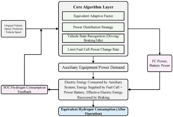
Figure 7.
Structural diagram of energy management strategy.
4.2. Comparison of Simulation Results
Figure 8 shows the SOC (battery state of charge) variation characteristics of the dynamic programming (DP) strategy, the Improved Adaptive Equivalent Consumption Minimization Strategy (P-ECMS), and the basic A-ECMS strategy under two driving cycles. Subfigure (a) corresponds to the C-WTVC (China World Transient Vehicle Cycle, China’s heavy-duty commercial vehicle transient cycle), and Subfigure (b) corresponds to the NREL2VAIL (National Renewable Energy Laboratory 2 Vehicle Advanced Investigation Laboratory, the U.S. National Renewable Energy Laboratory 2-type vehicle advanced research cycle), with a driving distance of 42.5 km. Under both cycles, the DP strategy achieves the best SOC stability, with variances as low as 8.08 × 10⁻⁶ and 1.81 × 10⁻⁶, respectively. The SOC fluctuation of P-ECMS remains within a controllable range, maintaining good battery charge stability in both short-cycle and long-distance operations. In contrast, the basic A-ECMS exhibits relatively more significant SOC fluctuations in the later stage.
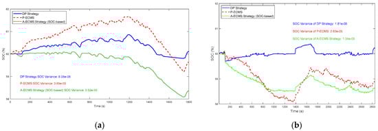
Figure 8.
Comparison of SOC fluctuations for three control strategies: (a) SOC comparison plot under the C-WTCV drive cycle; (b) SOC comparison plot under the NREL2VAIL drive cycle.
These two distinct driving cycles are selected for testing primarily to verify the generalization and adaptability of the strategies. The results show that all three strategies meet the SOC range control requirements. Among them, the DP strategy delivers the best stability performance, while P-ECMS (an improved strategy based on A-ECMS) maintains good SOC stability across different driving scenarios. This fully demonstrates the effectiveness of the improvements made to the A-ECMS strategy.
Figure 9 presents a detailed power distribution diagram for the energy management strategy of a fuel cell commercial vehicle, offering a clear visualization of the dynamic interaction between multiple energy sources. The various curves in the figure correspond to key energy flows, including total power demand, driving demand, net output of the fuel cell, traction battery power, and auxiliary system power. From the perspective of energy supply and demand logic, the total power on the demand side consists of two components: first, the driving demand power required for vehicle operation and overcoming resistance; second, the power needed to sustain on-board electrical equipment. On the supply side, the fuel cell acts as the core energy source (its output power is represented by the blue curve), while the traction battery (green curve) plays a role in peak shaving and valley filling. When total demand exceeds the fuel cell’s output, the traction battery discharges to supplement energy; when the fuel cell produces surplus power, the traction battery receives this excess for charging. The charging status of the traction battery is as shown in Figure 10.
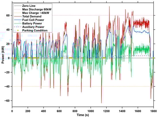
Figure 9.
Power distribution diagram.
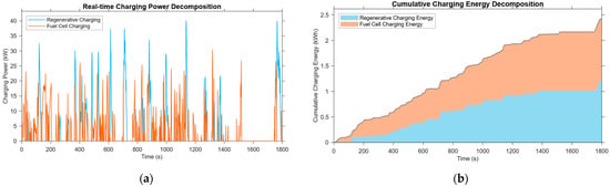
Figure 10.
Energy sources for traction battery charging: (a) charging power time series; (b) cumulative charging energy decomposition.
It should be noted that when the total demand is negative, the system enters a braking and deceleration process. The traction battery limiting its maximum charging power is not merely about restricting the motor’s regenerative capacity; rather, it stems from considerations of balancing braking safety and energy recovery. After all, in engineering practice, it is impossible for the motor to bear all braking torque alone—part of the required braking force must be provided by mechanical braking. Overall, through the dynamic matching of the fuel cell’s net output and the traction battery’s power, the system ensures that their sum remains balanced with the total demand power. This clearly demonstrates the energy collaboration characteristics of the multi-energy system under dynamic operating conditions, as well as the actual impact of the traction battery’s charging and discharging constraints on energy flow.
Considering the characteristics of power change rate and fluctuation frequency, in low-power operating conditions—such as when the vehicle is idling at intersections (as illustrated in Figure 11)—the traction battery is only required to support minor auxiliary loads, including vehicle lighting and air conditioning systems. During such periods, the fuel cell system is deactivated, and the traction battery operates independently to supply the necessary power. This approach not only conforms to the dynamic response capabilities of the battery in handling high-frequency, low-energy micro-power fluctuations—where small-amplitude variations can adequately meet load demands with a negligible impact on battery cycle life—but also prevents the fuel cell from operating in its inefficient low-load region. By exploiting the traction battery’s superior adaptability to low-frequency, low-amplitude, and transient power demands, the proposed strategy enhances overall energy utilization efficiency and effectively reduces equivalent hydrogen consumption. This operational logic clearly illustrates the synergistic advantages inherent in the parallel hybrid architecture: the fuel cell is optimized for stable, continuous power delivery to meet low-frequency, high-energy demands, whereas the traction battery provides agile, responsive support for high-frequency, low-power transients.
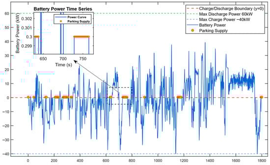
Figure 11.
Output power diagram of traction battery.
Figure 12 illustrates the operation process of the energy management strategy for fuel cell commercial vehicles via five subfigures.
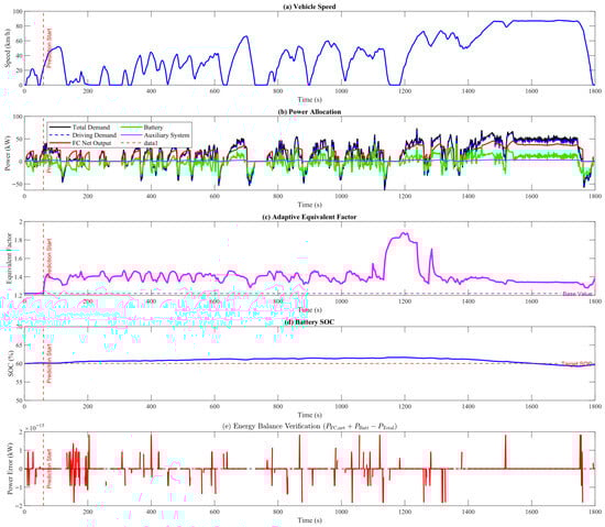
Figure 12.
Comprehensive diagram of energy management strategy.
Subfigure (a) shows the vehicle speed variation, which serves as the input condition for the operating cycle; Subfigure (b) demonstrates the power distribution logic, where the total demand power includes the vehicle driving power demand and auxiliary system power demand—as the main energy source, the fuel cell primarily operates in the 15–40 kW efficient range (where its energy efficiency is relatively high), while the power battery supplements or stores energy through “peak shaving and valley filling” to cooperate with the fuel cell in meeting the total demand; Subfigure (c) presents the dynamic changes in the adaptive equivalent factor, whose control logic first divides vehicle speed into three intervals (low, medium, high) with corresponding base values for the fuel cell output proportion (highest at high speed, followed by medium speed, lowest at low speed)—the equivalent factor does not independently regulate power but performs dynamic fine-tuning on the base proportion of the corresponding interval, so it fluctuates but does not rise significantly during the high-speed stage and remains within the preset range to adapt to operating conditions; Subfigure (d) shows that the battery SOC stays stable at medium and low speeds but decreases at high speeds due to the higher power demand and the lack of regenerative braking energy recovery; finally, Subfigure (e) verifies the model’s energy conservation accuracy, with the numerical calculation error in the order of 10−15 kW, indicating that the model strictly complies with energy conservation logic at the theoretical level.
- ➀
- Linear Correlation Formula for Fuel Cell Power and Hydrogen Consumption Rate.
As can be seen from Figure 13, the real-time hydrogen consumption rate of the fuel cell has a linear correlation with its output power , and its linear formula is as follows:
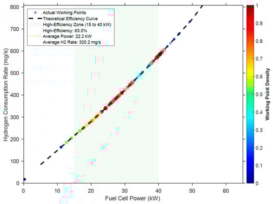
Figure 13.
Operating characteristic distribution diagram of fuel cell.
In Equation (30), is the FC power-hydrogen consumption slope, with the unit of g/(kW·h), and is the fuel cell idle hydrogen consumption, with the unit of g/h.
Figure 13 shows the distribution of the fuel cell’s operating characteristics. The redder the color of the scattered points, the higher the density of the operating points. Its operating points are mainly concentrated in the 15–40 kW range, which is the high-efficiency zone in the figure, accounting for 63.0%, corresponding to an average power of 22.2 kW and an average hydrogen consumption of 320.2 mg/s. The operating point density is lower in the intervals below 15 kW or above 40 kW, indicating that the adopted energy management strategy enables the fuel cell to operate more in the high-efficiency zone, thereby enhancing its energy utilization efficiency.
As shown in Figure 14, the DP strategy, a theoretical benchmark, results in high-frequency and large-amplitude oscillations in the fuel cell’s output power, with abrupt large-amplitude power jumps occurring instantaneously. Such aggressive power fluctuations are only feasible under ideal conditions and cannot be realized in practical applications, failing to meet the operational requirements of commercial vehicles. Thus, it can only serve as a theoretical reference for strategy optimization.
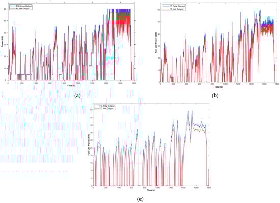
Figure 14.
Comparison chart of fuel cell output power: (a) DP fuel cell output power; (b) A-ECMS fuel cell output power; (c) P-ECMS fuel cell output power.
The traditional A-ECMS strategy lacks future operating condition prediction capability and relies solely on real-time feedback to adjust the equivalent factor. This causes frequent high-frequency and large-amplitude jumps in the fuel cell’s output power. When the vehicle undergoes abrupt changes in operating states (e.g., sudden acceleration or sharp deceleration), the fuel cell power exhibits immediate sharp rises and drops. Such unstable power output prevents the fuel cell from stably operating in its high-efficiency region, forcing it to operate in the low-efficiency range for longer periods. Consequently, this not only increases hydrogen consumption but also leads to the unsatisfactory control performance of the strategy.
To address the issue of high-frequency and large-amplitude jumps in fuel cell power under traditional strategies, the upper limit of the power change rate is first restricted to prevent sudden large power changes. On this basis, the P-ECMS strategy dynamically adjusts the equivalent factor based on vehicle speed prediction, further making the fuel cell power output more stable and the distribution more in line with changes in working conditions. In actual operation, its power is strongly correlated with vehicle speed, with smooth fluctuations and no random jumps, and can be stably maintained in the efficient working area. Compared with the dense and high-frequency jumps in Figure 14b, the fuel cell power curve under this strategy (as shown in Figure 15) fluctuates smoothly, with the fluctuation frequency significantly reduced. Although its hydrogen consumption is slightly higher than that of the DP strategy, due to stable operation in the efficient zone, the equivalent hydrogen consumption is much lower than that of the traditional A-ECMS, with outstanding energy-saving effects and an overall better performance.
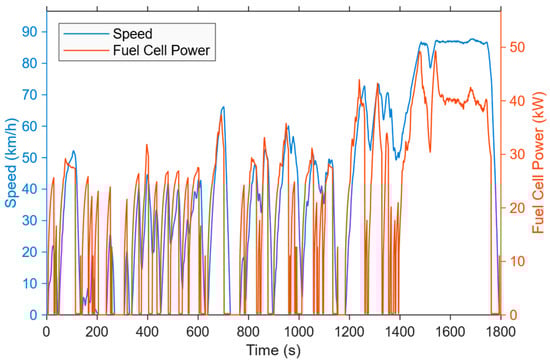
Figure 15.
Relationship between vehicle speed and fuel cell power.
Table 8 and Figure 16 present the equivalent hydrogen consumption and battery state-of-charge (SOC) data for the three strategies under the C-WTVC and NREL2VAIL conditions—all are initialized with an SOC of 0.60, but their performances differ significantly. The traditional A-ECMS exhibits 498.6 g of equivalent hydrogen consumption under C-WTVC, 10.5% higher than that of dynamic programming (DP, 451.2 g); under NREL2VAIL, its consumption reaches 1114.4 g, 13.2% higher than DP’s 984.5 g, alongside the fastest growth rate and the largest final SOC deviation from the initial value.
Table 8.
Equivalent hydrogen consumption.
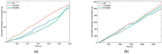
Figure 16.
Comparison chart of equivalent hydrogen consumption: (a) C-WTVC; (b) NREL2VAIL.
In contrast, the P-ECMS shows 480.6 g (6.5% higher than DP) under C-WTVC and 1053.3 g (7.0% higher than DP) under NREL2VAIL; its consumption is notably lower than the traditional A-ECMS, with more moderate growth and better final SOC stability. As the ideal optimal reference, DP maintains the lowest consumption across both conditions (final SOC nearly identical to the initial value), and the reasonable consumption gap between P-ECMS and DP, plus P-ECMS’s stable performance across conditions, demonstrates its favorable adaptability.
5. Conclusions
First, this study addresses a key limitation of the conventional Adaptive Equivalent Consumption Minimization Strategy (A-ECMS) for parallel fuel cell commercial vehicles under complex operating conditions—its one-dimensional control of the equivalent factor based solely on state-of-charge (SOC) deviation. Lacking the ability to predict future driving patterns, this approach suffers from response lag and exhibits poor adaptability to operating conditions. To resolve this, an improved Predictive Equivalent Consumption Minimization Strategy (P-ECMS) is proposed. Leveraging high-precision vehicle speed prediction data generated by the Sparrow Search Algorithm–Long Short-Term Memory (SSA-LSTM) model, the strategy integrates SOC deviation and vehicle operation trends to establish a two-dimensional dynamic equivalent factor regulation mechanism. It also incorporates a time-decay weighting mechanism (exponential decay is selected via comparative experiments on four typical decay functions to emphasize the weight of recent historical data), a MARC residual correction module, and a fused dynamic equivalent factor model—an integrated framework that resolves the response lag issue of traditional strategies and enables proactive adaptation to complex, varying operating conditions.
Second, following constrained hyperparameter tuning and feature enhancement, the improved SSA-LSTM model delivers a superior predictive performance. Outperforming the Gated Recurrent Unit (GRU) model, it boasts higher accuracy and better generalization across typical driving cycles (C-WTVC, NREL2VAIL, NYCTRUCK). This reliable forward-looking capability enables precise modulation of the dynamic equivalent factor and underpins advanced energy management optimization.
Simulation results confirm that, compared with conventional A-ECMS, the proposed P-ECMS reduces equivalent hydrogen consumption by 3.41% under C-WTVC and 5.48% under NREL2VAIL, while significantly improving SOC stability (with controllable fluctuation variance). By dynamically adjusting the equivalent factor, the strategy enhances the power battery’s “peak-shaving and valley-filling” capability—under harsh urban conditions like low-speed congestion and frequent start–stops, the power battery undertakes transient power demands, cushions start–stop impacts, and shares the fuel cell’s load, greatly reducing its frequent activation and abrupt power fluctuations. Ultimately, 63% of the fuel cell’s operating time is concentrated in the high-efficiency range, with its operating environment significantly improved. Quantitatively, the P-ECMS’s hydrogen consumption is only 6.5% (C-WTVC) and 7.0% (NREL2VAIL) higher than the globally optimal dynamic programming (DP) benchmark. By integrating hydrogen consumption optimization, SOC stability improvement, and better fuel cell operating conditions, it achieves good economic efficiency and excellent multi-condition adaptability.
Importantly, the P-ECMS supports the sustainable operation of fuel cell commercial vehicles through two key mechanisms. First, optimizing energy distribution to increase the fuel cell’s high-efficiency operating time enhances the hydrogen-to-electric conversion efficiency and reduces hydrogen consumption—enhancing economic viability and supporting the transportation sector’s decarbonization goals by promoting efficient zero-carbon hydrogen energy utilization. Second, dynamic equivalent factor adjustment enables flexible power allocation between the fuel cell and battery; under extreme conditions, the battery assumes more transient load and buffering tasks, alleviating fuel cell stress and reducing performance degradation. This extends the lifespan of critical components, lowers vehicle lifecycle resource consumption, and balances operational economy with long-term durability.
In future work, in-depth research will be conducted on the impact of the strategy on the lifespan of fuel cells and power batteries. The findings of this research will provide robust technical support for the operation of low-consumption, long-duration fuel cell commercial vehicles, facilitating the widespread application of fuel cell technology in transportation.
Author Contributions
Conceptualization, Y.W., W.Z., and J.Q.; methodology, Y.W. and W.Z.; software, Y.W. and W.Z.; investigation, Y.W. and W.Z.; data curation, Y.W. and W.Z.; writing—original draft preparation, Y.W.; writing—review and editing, Y.W., W.Z., and J.Q.; project administration, W.Z. and J.Q. All authors have read and agreed to the published version of the manuscript.
Funding
The work was funded by the Central Guidance for the Innovation-Driven Development Special Fund Project of Guangxi [Grant Nos. GuikeZY23055014, GuikeAA23062073] and Guangxi Transportation Science and Technology Promotion Project (GXJT-ZDSYS-2023-03-03). The funders had no role in the design of this study; in the collection, analyses, or interpretation of data; in the writing of the manuscript; or in the decision to publish the results. The remaining authors declare that this research was conducted in the absence of any commercial or financial relationships that could be construed as potential conflicts of interest.
Institutional Review Board Statement
Not applicable.
Informed Consent Statement
Not applicable.
Data Availability Statement
The original contributions presented in this study are included in the article. Further inquiries can be directed to the corresponding author.
Conflicts of Interest
Author Jirong Qin is employed by Dongfeng Liuzhou Motor Co., Ltd. The research framework, proposed strategy, and data analysis ideas in this study were independently developed by Yiming Wu and Weiguang Zheng. Jirong Qin’s contributions to this study—all limited to theoretical-level collaborative discussions based on his personal experience, and unrelated to any resources or technologies of his employer—include discussing the preliminary research framework, analyzing the feasibility of the proposed strategy, exchanging ideas regarding Section 3.5 and Section 4.2 (where control group data comparison and performance analysis are presented), and providing revision suggestions for the manuscript.
Abbreviations
| A-ECMS | Adaptive Equivalent Hydrogen Consumption Minimization Strategy |
| P-ECMS | Predictive Equivalent Hydrogen Consumption Minimization Strategy |
| SSA | Sparrow Search Algorithm |
| LSTM | Long Short-Term Memory Network |
| MARC | Moving Average Residual Correction Technique |
| GRU | Gated Recurrent Unit |
| DP | Dynamic Programming |
| PMP | Pontryagin’s Minimum Principle |
| ECMS | Equivalent Fuel Consumption Minimization Strategy |
| EMS | Energy Management Strategy |
References
- Energieagentur, I. Global Hydrogen Review 2023; OECD Publishing: Paris, France, 2023; Available online: https://www.oecd.org/en/publications/global-hydrogen-review-2023_cb2635f6-en.html (accessed on 15 October 2025).
- Howarth, R.W.; Jacobson, M.Z. How green is blue hydrogen? Energy Sci. Eng. 2021, 9, 1676–1687. [Google Scholar] [CrossRef]
- Offer, G.J.; Howey, D.; Contestabile, M.; Clague, R.; Brandon, N. Comparative analysis of battery electric, hydrogen fuel cell and hybrid vehicles in a future sustainable road transport system. Energy Policy 2010, 38, 24–29. [Google Scholar] [CrossRef]
- Wang, X. Review and Outlook of Fuel Cell Power Systems for Commercial Vehicles, Buses, and Heavy Trucks. Sustainability 2025, 17, 6170. [Google Scholar] [CrossRef]
- Yang, T.F.; Sheu, B.H.; Ghalambaz, M.; Yan, W.M. Effects of operating parameters and load mode on dynamic cell performance of proton exchange membrane fuel cell. Int. J. Energy Res. 2021, 45, 2474–2487. [Google Scholar] [CrossRef]
- Pukrushpan, J.T.; Stefanopoulou, A.G.; Peng, H. Control of fuel cell power systems: Principles, modeling, analysis and feedback design; Springer Science & Business Media: Berlin/Heidelberg, Germany, 2004. [Google Scholar]
- Guo, J.; He, H.; Jia, C.; Guo, S. The Energy Management Strategies for Fuel Cell Electric Vehicles: An Overview and Future Directions. World Electr. Veh. J. 2025, 16, 542. [Google Scholar] [CrossRef]
- Du, C.; Huang, S.; Jiang, Y.; Wu, D.; Li, Y. Optimization of energy management strategy for fuel cell hybrid electric vehicles based on dynamic programming. Energies 2022, 15, 4325. [Google Scholar] [CrossRef]
- Jia, C.; Qiao, W.; Cui, J.; Qu, L. Adaptive model-predictive-control-based real-time energy management of fuel cell hybrid electric vehicles. IEEE Trans. Power Electron. 2022, 38, 2681–2694. [Google Scholar] [CrossRef]
- Piras, M.; De Bellis, V.; Malfi, E.; Novella, R.; Lopez-Juarez, M. Hydrogen consumption and durability assessment of fuel cell vehicles in realistic driving. Appl. Energy 2024, 358, 122559. [Google Scholar] [CrossRef]
- Abduljabbar, R.L.; Dia, H.; Tsai, P.-W.; Liyanage, S. Short-term traffic forecasting: An LSTM network for spatial-temporal speed prediction. Future Transp. 2021, 1, 21–37. [Google Scholar] [CrossRef]
- Zhang, J.; Qu, S.; Zhang, Z.; Cheng, S. Improved genetic algorithm optimized LSTM model and its application in short-term traffic flow prediction. PeerJ Comput. Sci. 2022, 8, e1048. [Google Scholar] [CrossRef] [PubMed]
- Zhang, Y.; Gao, M.; Hua, G.; Xie, Q.; Guo, Y.; Zheng, R. Multisource Fusion of Exogenous Inputs Based NARXs Neural Network for Vehicle Speed Prediction between Urban Road Intersections. Proc. Inst. Mech. Eng. Part D J. Automob. Eng. 2024, 238, 3748–3759. [Google Scholar] [CrossRef]
- Kim, D.; Cho, Y.; Kim, D.; Park, C.; Choo, J. Residual correction in real-time traffic forecasting. In Proceedings of the 31st ACM International Conference on Information & Knowledge Management, Atlanta, GA, USA, 17–21 October 2022; pp. 962–971. [Google Scholar] [CrossRef]
- Pahon, E.; Péra, M.-C.; Bouquain, D.; Hissel, D. Impact of current ripples on the durability of proton exchange membrane fuel cells based on two ageing datasets. Data Brief 2022, 45, 108601. [Google Scholar] [CrossRef] [PubMed]
- Padgett, E.; Yarlagadda, V.; Holtz, M.E.; Ko, M.; Levin, B.D.; Kukreja, R.S.; Ziegelbauer, J.M.; Andrews, R.N.; Ilavsky, J.; Kongkanand, A. Mitigation of PEM fuel cell catalyst degradation with porous carbon supports. J. Electrochem. Soc. 2019, 166, F198–F207. [Google Scholar] [CrossRef]
- Zaidi, S.M.H. Unsupervised classification of multi-class chart images: A comparison of customized CNNs and transfer learning techniques. PeerJ Comput. Sci. 2025, 11, e3148. [Google Scholar] [CrossRef]
- Topić, J.; Škugor, B.; Deur, J. Synthesis and feature selection-supported validation of multidimensional driving cycles. Sustainability 2021, 13, 4704. [Google Scholar] [CrossRef]
- Krichen, M. Long Short-Term Memory Networks: A Comprehensive Survey. AI 2025, 6, 215. [Google Scholar] [CrossRef]
- Wang, W.; Zhang, K.; Zhang, Q.; Wang, X. Research on energy management strategy for incremental range electric vehicles integrating speed prediction. Sci. Prog. 2025, 108, 368504241308957. [Google Scholar] [CrossRef]
- Tabatabaei, S.M. Well placement optimization with a novel swarm intelligence optimization algorithm: Sparrow Search Algorithm. Geoenergy Sci. Eng. 2023, 231, 212291. [Google Scholar] [CrossRef]
- Shi, F.; Wang, Y.; Chen, J.; Wang, J.; Hao, Y.; He, Y. Short-term vehicle speed prediction by time series neural network in high altitude areas. In IOP Conference Series: Earth and Environmental Science; IOP Publishing: Bristol, UK, 2019; p. 032072. [Google Scholar] [CrossRef]
- Huang, X. Combined use of long short-term memory neural network and quantum computation for hierarchical forecasting of locational marginal prices. Energy Convers. Econ. 2025, 6, 26–38. [Google Scholar] [CrossRef]
- Mozaffari, L.; Mozaffari, A.; Azad, N.L. Vehicle speed prediction via a sliding-window time series analysis and an evolutionary least learning machine: A case study on San Francisco urban roads. Eng. Sci. Technol. Int. J. 2015, 18, 150–162. [Google Scholar] [CrossRef]
- Chughtai, J.-u.-R.; Haq, I.U.; Muneeb, M. An attention-based recurrent learning model for short-term travel time prediction. PLoS ONE 2022, 17, e0278064. [Google Scholar] [CrossRef]
- Xie, H.; Zhang, Y.; He, Y.; You, K.; Fan, B.; Yu, D.; Lei, B.; Zhang, W. Parallel attention-based LSTM for building a prediction model of vehicle emissions using PEMS and OBD. Measurement 2021, 185, 110074. [Google Scholar] [CrossRef]
- Ouyang, T.; Zha, X.; Qin, L.; He, Y.; Tang, Z. Prediction of wind power ramp events based on residual correction. Renew. Energy 2019, 136, 781–792. [Google Scholar] [CrossRef]
- Baghoussi, Y.; Soares, C.; Mendes-Moreira, J. Corrector LSTM: Built-in Training Data Correction for Improved Time-Series Forecasting. Neural Computing and Applications 2024, 36, 16213–16231. [Google Scholar] [CrossRef]
- Zhang, Y. Vehicle Dynamics Estimator Utilizing LSTM-Ensembled Adaptive Kalman Filter. IEEE Trans. Ind. Electron. 2025, 72, 5429–5439. [Google Scholar] [CrossRef]
- Lin, X. Stochastic velocity-prediction conscious energy management strategy based self-learning Markov algorithm for a fuel cell hybrid electric vehicle. Energy 2025, 320, 135167. [Google Scholar] [CrossRef]
- Jia, C. Health-conscious energy management for fuel cell vehicles: An integrated thermal management strategy for cabin and energy source systems. Energy 2025, 333, 137330. [Google Scholar] [CrossRef]
- Khalatbarisoltani, A.; Zhou, H.; Tang, X.; Kandidayeni, M.; Boulon, L.; Hu, X. Energy management strategies for fuel cell vehicles: A comprehensive review of the latest progress in modeling, strategies, and future prospects. IEEE Trans. Intell. Transp. Syst. 2023, 25, 14–32. [Google Scholar] [CrossRef]
- He, K.; Qin, D.; Chen, J.; Wang, T.; Wu, H.; Wang, P. Adaptive equivalent consumption minimization strategy for fuel cell buses based on driving style recognition. Sustainability 2023, 15, 7781. [Google Scholar] [CrossRef]
- Zhou, Y. Speed-prediction-based hierarchical energy management and operating cost analysis for fuel cell hybrid logistic vehicles. Appl. Energy 2025, 390, 125843. [Google Scholar] [CrossRef]
- Gao, D.; Jin, Z.; Lu, Q. Energy management strategy based on fuzzy logic for a fuel cell hybrid bus. J. Power Sources 2008, 185, 311–317. [Google Scholar] [CrossRef]
- Sicilia, M.; Cervone, D.; Polverino, P.; Pianese, C. Adaptive Equivalent Consumption Minimization Strategies for Plug-in Hybrid Electric Vehicles: A Review. Energies 2025, 18, 5475. [Google Scholar] [CrossRef]
Disclaimer/Publisher’s Note: The statements, opinions and data contained in all publications are solely those of the individual author(s) and contributor(s) and not of MDPI and/or the editor(s). MDPI and/or the editor(s) disclaim responsibility for any injury to people or property resulting from any ideas, methods, instructions or products referred to in the content. |
© 2025 by the authors. Licensee MDPI, Basel, Switzerland. This article is an open access article distributed under the terms and conditions of the Creative Commons Attribution (CC BY) license.