A Coupled SWAT-LSTM Approach for Climate-Driven Runoff Dynamics in a Snow- and Ice-Fed Arid Basin

Abstract

As global climate change intensifies, hydrological processes in arid inland river basins are undergoing profound transformations, posing severe challenges to regional water security and ecological stability. This study aims to develop a coupled SWAT-LSTM model integrating glacier melt processes to simulate runoff dynamics in the Keria River basin under climate change, providing a basis for local water resource management. Based on natural monthly runoff observations from the Langgan hydrological station (1961–2015), glacier data extracted from Landsat 8 remote sensing imagery (2013–2019), and downscaled data from the CMIP6 Multi-Model Ensemble (MME), this study constructed a SWAT-LSTM coupled model to simulate future scenarios (2026–2100). Research indicates that this hybrid model significantly enhances the accuracy of hydrological simulations in high-altitude glacier-fed catchments. The Nash efficiency coefficient (NSE) during the validation period reached 0.847, representing a 15% improvement over the SWAT model. SSP5-8.5 is identified as a high-risk scenario, underscoring the urgency of emissions reduction; SSP1-2.6 represents the most desirable pathway, with its relatively stable pattern offering sustained advantages for long-term water resource management in the basin. The study further reveals a negative feedback mechanism between glacier ablation and runoff increase, validating the regulatory role of Jiyin Reservoir’s “store during floods to compensate for droughts” operation strategy in balancing basin water resources. This study explores the coupling path between the physical model and the deep learning model, and provides an effective integration scheme for the hydrological simulation of the global watershed with ice–snow meltwater as the main recharge runoff, especially for the adaptive management of water resources in inland river basins in arid areas.

1. Introduction

Anthropogenic climate change stands as a defining scientific challenge confronting global society in the current century [1]. It is established in the IPCC Sixth Assessment Report (AR6) that a global surface temperature increase of 0.52–0.92 °C has occurred over the period spanning from 1850 to the present. By the end of this century (using 1980–1999 as the baseline period), global average surface temperatures are projected to increase by an additional 1.1–6.4 °C [2]. This pronounced warming trend has profoundly impacted global hydrological processes, leading to significant changes in key hydrological elements such as temperature, precipitation, evapotranspiration, and runoff [3]. This reconfiguration of spatiotemporal hydrological patterns is directly manifested in the increased occurrence and intensity of extreme events like droughts and floods. These changes pose dual challenges: complicating hydrological modeling and forecasting, and jeopardizing long-term societal sustainability.

In hydrological research, hydrological models serve as vital tools for revealing the patterns of runoff evolution [4]. Traditionally, process-based models (PBMs) have become the mainstream approach for runoff simulation by constructing mathematical frameworks to systematically simulate watershed hydrological processes [5,6]. Among these, the semi-distributed SWAT model (Soil and Water Assessment Tool) is representative due to its widespread application in water resource assessment and nonpoint source pollution simulation [7,8]. However, such models feature numerous parameters and complex mechanisms, resulting in a time-consuming calibration process [9]. In recent years, machine learning (ML) algorithms represented by long short-term memory (LSTM) networks have increasingly become an effective complementary approach to hydrological modeling. They better capture the nonlinear characteristics of hydrological processes, with simulation accuracy surpassing traditional physical models in multiple aspects [10].

Nevertheless, both physical models and machine learning approaches rely heavily on high-quality observational data for runoff simulation. In data-scarce basins, physical models are prone to systematic biases, while machine learning models generally face challenges with insufficient generalization capabilities [11,12,13]. Therefore, the development of new methods such as transfer learning and parameter regionalization to improve the accuracy and robustness of runoff simulation in data-poor areas has become the key direction of current research. In this context, a new modeling strategy coupling process model and machine learning method, SWAT-LSTM, is proposed. This method employs SWAT-simulated hydrological process variables combined with meteorological driver data as input for the LSTM model, and its effectiveness has been successfully validated in China’s Jiulong River basin [14]. The construction and calibration of SWAT-LSTM coupling model essentially depend on high-precision and continuous meteorological data sequences. The structural characteristics of the model determine its high sensitivity to climate change. The SWAT module transforms climate factors such as temperature and precipitation into watershed hydrological processes through physical equations, while the LSTM module learns and captures the complex nonlinear relationship between these physical process variables, meteorological driving factors and runoff responses. Therefore, the simulation results of the model can directly reflect the impact of climate fluctuations and changes, and become a powerful tool for assessing the hydrological response to climate change. However, existing coupled model studies have primarily focused on data-rich mid-to-low latitude basins. When applied to arid mountainous watersheds that are highly dependent on glacier meltwater and highly sensitive to climate change, there are still significant defects: most models fail to adequately incorporate glacial hydrological processes and lack systematic validation in glacial basins with sparse data [14], with insufficient exploration of the coupling mechanisms between glacial melt modules and data-driven components. Furthermore, coupled models in such watersheds compromise the precise simulation of critical processes—such as flood peak timing—and struggle to effectively quantify the combined impacts of natural and human activities, including glacier retreat and reservoir regulation [15,16]. Therefore, developing coupled models that can effectively characterize glacier ablation processes and are applicable under data-scarce conditions is crucial for accurately simulating and predicting the hydrological responses of such vulnerable watersheds.

This study analyzes the Keriya River, a typical inland river in China’s arid northwest region. As a globally significant hotspot for water resource vulnerability, this basin shares high comparability with other arid inland rivers such as Central Asia’s Amu Darya, Africa’s Okavango, and North America’s Colorado River [17,18,19]. Its characteristics—dominated by glacial meltwater replenishment, regulated by upstream reservoirs, and ultimately flowing into desert terrain—are strikingly similar. The region exhibits precipitation variability and warming rates significantly higher than global averages, underscoring its extreme sensitivity to climate change [20,21]. Against this backdrop, water resources have become the key limiting factor sustaining the socio-ecological sustainability of endorheic basins. The glacier-covered mountainous regions upstream, serving as areas for runoff formation and water conservation, form an ecologically interdependent relationship with the water-consuming oases downstream—where water brings life to the oases, and its absence leads to desertification [22,23,24]. As the primary water source for the Yutian Oasis, Kriya River sustains agricultural irrigation, ecological balance, and domestic water supply within the region [25,26,27]. Meanwhile, the Jiyin Water Conservancy Project constructed at the headwaters of the Kriya River significantly regulates downstream runoff processes through cross-annual water storage and flood retention during the flood season. Therefore, studying runoff variations in the Kriya River basin not only helps reveal the response mechanisms of cold-region hydrological processes driven by climate, but also holds significant importance for deepening our understanding of the functions of mountain reservoirs in water resource regulation and ecological conservation [28].

Currently, when using the SWAT model to simulate snowmelt runoff, the lack of a glacier hydrology module limits simulation accuracy in modeling the hydrological processes of watersheds where snowmelt serves as the primary recharge source. So, how can this issue be addressed? Based on this, this study aims to construct and validate a hybrid SWAT-LSTM model coupled with a glacier ablation module to enhance the hydrological simulation capability of inland river basins in snow- and ice-fed arid regions. The research centers on the following three core scientific issues: (1) Whether the SWAT-LSTM coupled model possesses high-precision runoff simulation capabilities in basins dominated by glacial meltwater recharge; (2) The specific regulatory mechanisms and impact extent of Jiyin Reservoir operations on natural runoff processes; (3) Long-term runoff evolution trends and climate response characteristics in the basin from 2026 to 2100 under different Shared Socioeconomic Pathway (SSP) scenarios. The innovation of this study lies in establishing a dual-driven “physical-data” modeling framework. By incorporating a glacier module, it addresses the structural limitations of SWAT in simulating glacial hydrological processes observed in previous research. Furthermore, the integration of LSTM enhances the nonlinear fitting capability for complex runoff time series, enabling precise simulation of the synergistic effects of climate variability and glacial melt on runoff. Compared with existing studies, this paper not only systematically verifies the applicability of this hybrid model in glacial basins of arid regions but also further quantifies the impact of reservoir operations on runoff processes and conducts long-term runoff projections under multiple scenarios. The research findings provide scientific basis for water resource management in the Keriya River basin. Moreover, the proposed transferable modeling framework offers methodological guidance and practical reference for arid mountainous watersheds worldwide facing similar water crisis challenges.

2. Materials and Methods

2.1. Overview of the Study Area

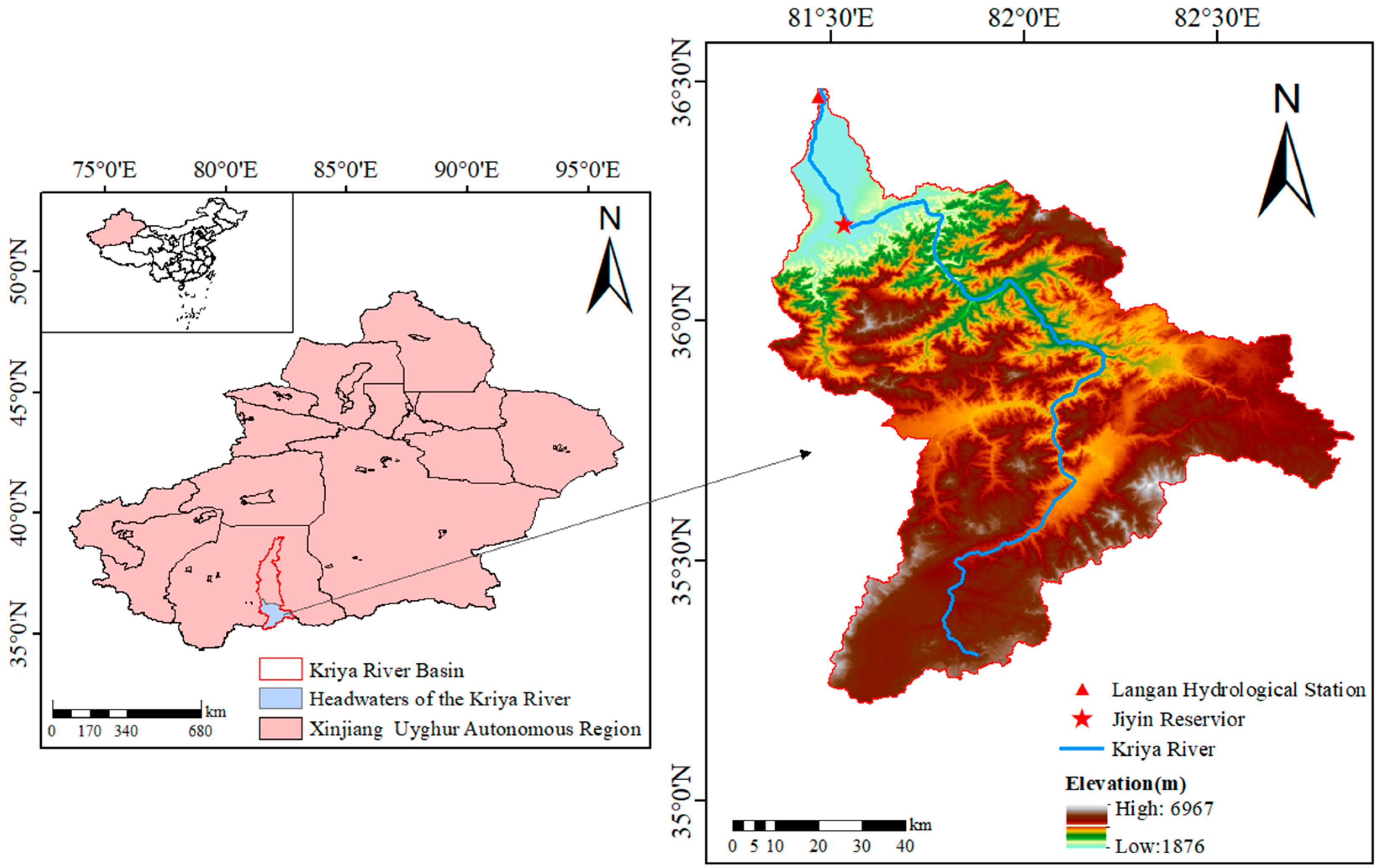
The Kriya River has its headwaters on the northern slopes of Usten Tagh, the highest peak of the Kunlun Mountains. Modern glaciers extensively develop in its headwaters, with the snowline ranging between 5600 and 5900 m. Glacial resources are vital to sustaining regional ecological balance and supporting socioeconomic development.

Geologically situated within the Western Kunlun Orogenic Belt, the headwaters region exhibits active neotectonic activity. The strong neotectonic movement has shaped its basic geomorphological pattern. The study area is mainly composed of Hercynian granodiorite. The lithology is light gray coarse-grained structure. The rock joints and fissures are relatively developed. The terrain cutting depth is 500–1000 m. This geological background controls the formation and collection process of surface runoff. Observations from 2001 to 2020 indicate that the mean annual areal coverage of the snowpack in the headwaters area is approximately 34%. Runoff recharge is primarily sourced from snowmelt and glacial meltwater, supplemented by summer rainfall and groundwater [29]. The study area is centered on the Langan hydrological station (81°28′10.26″ E, 36°27′58.45″ N) as the control section. Upstream lies the Jiyin Water Conservancy Project (81°32′ E, 36°12′ N), which began impoundment in September 2016 and fully completed by the end of 2018, exerting significant regulation on downstream runoff and flood processes. This study focuses on the headwaters upstream of the Langan station, where the watershed morphology approximates a triangle (Figure 1).

Figure 1. Overview of the source area of the Kriya River.

2.2. Data Sources and Processing

2.2.1. Data Sources

The fundamental data required for the study are detailed in Table 1. At the future data-driven level, seven major global climate models developed by leading institutions were selected from CMIP6 based on a comprehensive assessment of geographical representativeness, data availability, and existing research [30,31]. At the model construction level, the existing hydrological simulation framework was utilized to integrate multi-source spatial and observational data (including DEM, land use, soil, historical and future meteorological, and runoff data) [32].

Table 1. Research Data and Climate Modeling System.

Type	Content	Key Information
Spatial Data	DEM (30 m)	Geospatial Data Cloud (Generating River networks within basins and delineating sub-basins)
	Land Use Data (30 m)	Resource Environment Science and Data Center (Hydrological Response Unit Delineation)
	Soil Data (1:1,000,000)	Spatio-Temporal Tripolar Environmental Big Data Platform (Soil Database Construction)
	Landsat8 (30 m)	Google Earth Engine Platform (Glacier Area Extraction)
Meteorological and Hydrological Data	Historical Meteorological Data (Daily Values)	CN05.1 Dataset (Chinese Academy of Sciences Center for Climate Change Research)
	Actual Runoff Data (Monthly Values)	Langan Hydrological Station (1961–2019)
	Future Weather Data (Daily Values)	CMIP6 Official Website
Climate Model	7 CMIP6 GCMs	See details 1
Climate Scenario	SSP-1.26 (Low Coercivity)	A combination of low vulnerability, minimal mitigation pressure, and limited radiative forcing
	SSP-2.45 (Medium Compulsion)	Combination of Moderate Societal Vulnerability and Moderate Anthropogenic Radiative Forcing
	SSP-5.85 (High-Force)	The only shared socio-economic pathway achieving the 2100 anthropogenic radiative forcing target

¹ ACCESS-CM2 (Australia), BCC-CSM2-MR (China), CanESM5 (Canada), GFDL-ESM4 (United States), INM-CM4-8 (Russia), IPSL-CM6A-LR (France), and MPI-ESM1-2-LR (Germany).

2.2.2. Glacier Data Processing

Based on the Google Earth Engine (GEE) platform, the glacier distribution in the source region of the Keriya River was systematically extracted using Landsat 8 OLI/TIRS Collection 2 Tier 1 surface reflectance data from 2013 to 2019. In the preprocessing, QA_PIXEL band mask clouds and cloud shadows were used to screen qualified images with low cloud coverage during the strong ablation period each year. Glacier extraction adopts a conservative multi-threshold joint strategy: the normalized snow index (NDSI) is used as the core index to set the threshold for initial classification, and then the elevation and slope constraints derived from the SRTM digital elevation model (DEM) are introduced to eliminate the influence of low-altitude snow and steep terrain, supplemented by the normalized vegetation index (NDVI) threshold to suppress vegetation misclassification. In order to improve the stability of the results, a multi-temporal fusion strategy is used to retain only the pixels that are consistently identified as glaciers in most observations during the same ablation period, thereby generating an annual stable glacier distribution map. In the accuracy verification section, Randolph Glacier Inventory (RGI) V7.0 was used as the benchmark true value, and a series of indicators such as overall accuracy, accuracy, recall rate, F1-Score and Kappa coefficient were calculated by pixel-by-pixel comparison to comprehensively evaluate the reliability of the extraction results and provide a high-quality data basis for subsequent research.

2.3. Modeling Framework and Evaluation Methods

2.3.1. SWAT Model Description

The SWAT model, conceived by the USDA, is a distributed hydrological modeling framework for river basins that finds applications in diverse research areas including hydrological cycles, ecosystem dynamics, and land use management. This model can simulate and predict the effects of various watershed development configurations on hydrologic fluxes and contaminant transport, and has been extensively utilized in soil erosion assessment, agricultural planning, and management. Compared to traditional hydrological models, SWAT employs Hydrological Response Units (HRUs) as its fundamental simulation units. This approach effectively replaces complex grid-based calculations, significantly enhancing the efficiency of simulating long-term hydrological processes in large-scale watersheds while maintaining simulation accuracy. The SWAT simulation workflow primarily involves the following steps: First, extract the watershed river network and delineate sub-basins based on a digital elevation model. Next, integrate spatial data such as soil type, land use, and slope to further subdivide each sub-basin into Hydrological Response Units (HRUs) with homogeneous surface characteristics. Finally, calculate the hydrological flux for each HRU and simulate the runoff process of the main river through river network confluence. The hydrological processes in SWAT are governed by its fundamental water balance equation:

$$\begin{array}{c}\begin{array}{c}S{W}_t=S{W}_0+{\displaystyle \sum _{i=1}^n}(R_{day}-Q_{surf}-E_a-W_{seep}-Q_{gw})\end{array}\end{array}$$

(1)

In the equation, $S{W}_t$ is the final soil moisture content (mm); $S{W}_0$ is the pre-soil moisture content (mm); t is the time step (day); $R_{day}$ is the precipitation (mm); $Q_{surf}$ is the surface streamflow (mm); $E_a$ is the evapotranspiration (mm); $W_{seep}$ is the lateral flow and infiltration in the soil slope horizons (mm); $Q_{gw}$ and is the groundwater content (mm).

2.3.2. LSTM Model Description

Long Short-Term Memory (LSTM) belongs to the class of recurrent neural network (RNN) architectures renowned for their efficacy in sequence modeling tasks [33]. LSTM achieves precise control over information flow by incorporating memory units and gating mechanisms—including input gates, forget gates, cell state gates, and output gates—thereby enabling selective retention and discarding of information. This architecture allows LSTMs to effectively capture long-term dependencies in time series data, demonstrating advantages in numerous hydrological and climatological studies. To enhance the model’s predictive capability for extreme hydrological events, this study specifically designed a peak-sensitive dynamic weighted loss function:

$$\begin{array}{c}\mathcal{L}={\displaystyle \frac{1}{N}}{\displaystyle \sum _{i=1}^N}w\left(Q_i\right)\cdot {\left({\widehat{Q}}_i-Q_i\right)}^2\end{array}$$

(2)

The weighting function is based on a smooth distribution of traffic percentiles:

$$\begin{array}{c}w\left(Q_i\right)=1+\alpha \cdot sigmoid\left({\displaystyle \frac{Q_i-Q_{50\%}}{\beta }}\right)\end{array}$$

(3)

In the equation, $Q_i$ denotes the measured runoff volume, ${\widehat{Q}}_i$ represents the model’s predicted value, $Q_{50\%}$ is the median historical runoff, while α and β control peak sensitivity and weight smoothing, respectively. The parameters α and β in the peak sensitive loss function can be determined by grid search combined with K-fold cross-validation. With the goal of optimizing the comprehensive score of the overall fitting degree and the flood peak prediction ability at the same time, it is ensured that the parameter selection not only improves the capture accuracy of high flow events, but also maintains the overall performance balance of the model. This loss function employs an S-shaped activation function to enable continuous weight adjustment, ensuring high-flow events receive greater emphasis while maintaining training stability.

2.3.3. SWAT-LSTM Coupling Mechanism

This study developed a hybrid SWAT-LSTM hydrological model integrating physical mechanisms with deep learning [34,35]. Based on the bidirectional LSTM network and the self-attention mechanism, the model effectively captures the long-term dependencies and spatio-temporal features in runoff series, and enhances the feature propagation ability through residual connection. To address the physical constraints inherent in the SWAT model, a dual-path residual learning strategy is introduced to directly optimize the residuals between SWAT simulation values and observed data, ensuring flow conservation.

To overcome the structural limitations of the SWAT model in characterizing glacial hydrological processes, this study developed a simulation framework integrating physical mechanisms with data-driven approaches. By incorporating multi-source glacial data into an LSTM network, the framework effectively enhances simulation performance in high-altitude cold basins. It constructed a glacier ablation potential module based on the baseline glacier area and annual retreat rate data of the Keriya River obtained during the Third Xinjiang Scientific Expedition. It integrated 30-m resolution glacier distribution information extracted from Landsat 8 remote sensing imagery covering 2013–2019. A degree-day factor model was employed to dynamically calculate monthly ablation potential and cumulative ablation volume during the ablation period, which served as key features input into the LSTM model. During the model validation phase, the study generated monthly area time series by interpolating annual average glacier area data. This approach enabled a systematic comparison and validation of simulated runoff results between the SWAT-LSTM coupled model and the standalone SWAT model. To enhance the reliability and physical consistency of monthly-scale ablation data, the interpolation process employs the MODIS snow cover product (MOD10A2) as a dynamic constraint and utilizes a time-weighted averaging method to calibrate seasonal fluctuations. This method effectively captures the pronounced seasonal characteristics of glacial melt by incorporating high-frequency sequential snow data as a weighting factor, ensuring spatiotemporal consistency of the data. It not only overcomes the inherent bias of linear interpolation in characterizing nonlinear hydrological processes but also more accurately reflects the physical mechanisms of glacial melt. Simultaneously, it generates spatiotemporally consistent, numerically smoothed monthly-scale sequences, significantly reducing data noise and uncertainty. Ultimately, this study employs systematic data fusion and processing methods to provide reliable inputs for hydrological modeling in glacier-fed arid and semi-arid river basins, thereby enhancing the applicability and forecasting capabilities of the model [36,37].

The model system integrates multi-source heterogeneous data to establish a physically constrained glacier hydrological prediction framework, with the overall workflow depicted in Figure 2. Model inputs include meteorological elements (daily precipitation, maximum/minimum temperatures), SWAT model outputs (simulated runoff, evapotranspiration, snowmelt volume), and monthly-scale ablation potential and cumulative ablation characteristics dynamically calculated using the Kriya River glacier area baseline and annual retreat rate through a degree-day factor model [38]. During the data preprocessing stage, db4 wavelet adaptive threshold denoising, high-order feature cross-correlation, and two-stage feature selection are employed to enhance input representation capabilities. The core model comprises a feature fusion module employing a bidirectional two-layer LSTM (64 hidden units) to extract temporal features. These features undergo BatchNorm and Dropout (0.5) regularization, with a 16-head attention mechanism introduced to focus on critical hydrological events. A fully connected layer then implements residual connections. To embed hydrological physics, the model innovatively incorporates a dual-path residual learning structure with mass balance constraints, ensuring synthetic runoff adheres to water balance principles. During training, a dynamic weighted loss function is employed alongside learning rate warm-up and cosine annealing scheduling strategies, with early stopping optimized for model generalization [39,40,41,42]. Ultimately, the coupled model was trained using 1964–1999 data and validated with 2000–2015 data, maintaining consistent time-period segmentation with the SWAT model to achieve precise runoff predictions.

Figure 2. Architecture of the Coupled SWAT-LSTM Method.

2.3.4. Model Evaluation Metrics

This study employs the Nash efficiency coefficient (NSE), coefficient of determination (R²), percentage bias (PBIAS), root mean square error (RMSE), and mean absolute error (MAE) to comprehensively evaluate the effectiveness of runoff simulation. These metrics are calculated by comparing simulated values with observed values, thereby systematically evaluating the model’s performance in flow forecasting. NSE is used to evaluate the performance of hydrological models, as shown in Formula (4). When the NSE value approaches 1, it indicates that the simulated values closely match the observed target values. R² reflects the proportion of variance in observed values explained by simulated values, with values ranging from 0 to 1, as shown in Formula (5). A higher R² value indicates a stronger correlation between simulated and observed values. PBIAS represents the percentage deviation between simulated and measured values, as shown in Formula (6). The closer its absolute value is to zero, the better the model’s simulation performance. RMSE is a measure of the average squared difference between target values, simulated values, and observed values, as shown in Formula (7). A lower RMSE value indicates superior model output, and values closer to zero signify smaller prediction errors. MAE is the mean absolute error between the target value and the observed target value, as shown in Formula (8). A lower MAE value indicates smaller prediction errors, signifying better model performance [43,44]. Generally, simulation results are considered satisfactory when R² > 0.6 and NSE > 0.5 [45]. PBIAS > 0 indicates that the simulated value is smaller than the observed value; conversely, the simulated value is larger [46].

$$\begin{array}{c}NSE=1-{\displaystyle \frac{{\displaystyle {\sum }_{i=1}^n}{\left(y_i-x_i\right)}^2}{{\displaystyle {\sum }_{i=1}^n}{\left(y_i-\overline{y}\right)}^2}}\end{array}$$

(4)

$$\begin{array}{c}{R}^2={\displaystyle \frac{{\left[{\displaystyle {\Sigma }_{i=1}^n}\left(x_i-\overline{x}\right)\left(y_i-\overline{y}\right)\right]}^2}{{\displaystyle {\sum }_{i=1}^n}{\left(x_i-\overline{x}\right)}^2{\displaystyle {\sum }_{i=1}^n}{\left(y_i-\overline{y}\right)}^2}}\end{array}$$

(5)

$$\begin{array}{c}PBIAS={\displaystyle \frac{{\displaystyle {\Sigma }_{i=1}^n}\left(x_i-y_i\right)}{{\displaystyle {\Sigma }_{i=1}^n}{y}_i}}\times 100\end{array}$$

(6)

$$\begin{array}{c}RMSE=\sqrt{{\displaystyle \frac{{\displaystyle {\sum }_{i=1}^n}{\left(y_i-x_i\right)}^2}{n}}}\end{array}$$

(7)

$$\begin{array}{c}MAE= {\displaystyle \frac{{\displaystyle {\sum }_{i=1}^n}\left|y_i-{x_i}_i\right|}{n}}\end{array}$$

(8)

In the equation, $x_i$ and $y_i$ represent simulated and observed runoff, respectively; $\overline{x}$ and $\overline{y}$ denote the mean values of simulated and observed runoff, respectively; and n is the time period.

2.4. CMIP6 Data Processing

2.4.1. Downscaling and Bias Correction

GCM output data exhibit low resolution and variations in spatial resolution, and their direct application to the SWAT model can significantly impact results. To scientifically select reliable future climate scenarios, this study first conducted a comprehensive assessment of the model performance of multiple CMIP6 models. Based on this assessment, seven models were selected for subsequent analysis (See Table 1 for Climate Model). Model selection criteria comprehensively considered the following factors: (1) model participation in relevant international initiatives (e.g., ScenarioMIP) and data availability; (2) model performance in simulating the climate of arid Central Asia, particularly extreme precipitation and temperature variations [30,31]; (3) model independence to represent the full range of uncertainty in future climate projections. Based on this evaluation, seven CMIP6 climate models were ultimately selected for subsequent analysis.

Based on this, statistical downscaling was employed to downscale daily temperature and precipitation data from the baseline interval (1975–2014) and projection horizon (2026–2100) outputs of seven CMIP6 climate models onto 30 grid points corresponding to observed data. Subsequently, the Delta method is applied to perform station-specific bias correction on the daily temperature and precipitation data [47,48]. For temperature scenario calculations, the rate of change is measured using absolute change. By comparing the monthly mean temperatures of the future period and the baseline period from each GCM output, the absolute change is calculated. This change is then added to the observed temperatures at grid-cell stations to obtain the temperatures for the future period [49]. The temperature correction equation is:

$$\begin{array}{c}{T}_d=T_{obs,d}+\left(T_{obs,m}-T_{sim,m}\right)\end{array}$$

(9)

In the equation, $T_d$ is the revised daily temperature (°C), $T_{obs,d}$ is the daily observed temperature (°C), $T_{obs,m}$ is the calculated monthly average temperature values (°C), and $T_{sim,m}$ represents the climate monthly average temperature values (°C).

For the calculation of downscaling and bias revisions for precipitation scenarios, based on the output of future period data from each GCM grid, the mean value is compared with the GCM grid base period mean to obtain the proportion of change, and then this proportion is multiplied by the base period observations of each meteorological station to obtain the amount of change during the future phase [50]. The revised formula for precipitation is:

$$P_d=P_{sim,d}{\displaystyle \frac{P_{obs,m}}{P_{sim,m}}}$$

(10)

In the equation, $P_d$ is the revised daily precipitation (mm), $P_{sim,d}$ is the climate model daily precipitation (mm); $P_{obs,m}$ and $P_{sim,m}$ are the average monthly precipitation (mm) for the observation month and climate model.

2.4.2. Climate Model Performance Evaluation

CMIP6 climate models’ evaluation primarily focused on their ability to simulate historical climate elements (such as temperature and precipitation) in the study area, emphasizing consistency with observational data in spatial distribution, seasonal variations, and interannual variability. A comprehensive assessment of the performance of seven models from the CMIP6 archive alongside their ensemble mean (MME) was conducted using Taylor’s graphical method [51]. This diagram visually compares the simulation capabilities of each model across three dimensions: The position of the standardized standard deviation on the horizontal axis reflects the model’s ability to capture climate variability, with 1.0 representing perfect agreement with observed variability. In a Taylor diagram, the CRMSE for a given model simulation can be determined by measuring the dashed radial distance from the model’s position to the reference point (‘Observed’) located on the x-axis. The closer the point is to the origin, the smaller the systematic bias and the better the simulation performance [52].

3. Results and Discussion

3.1. Model Construction and Performance Analysis

3.1.1. SWAT Model Construction

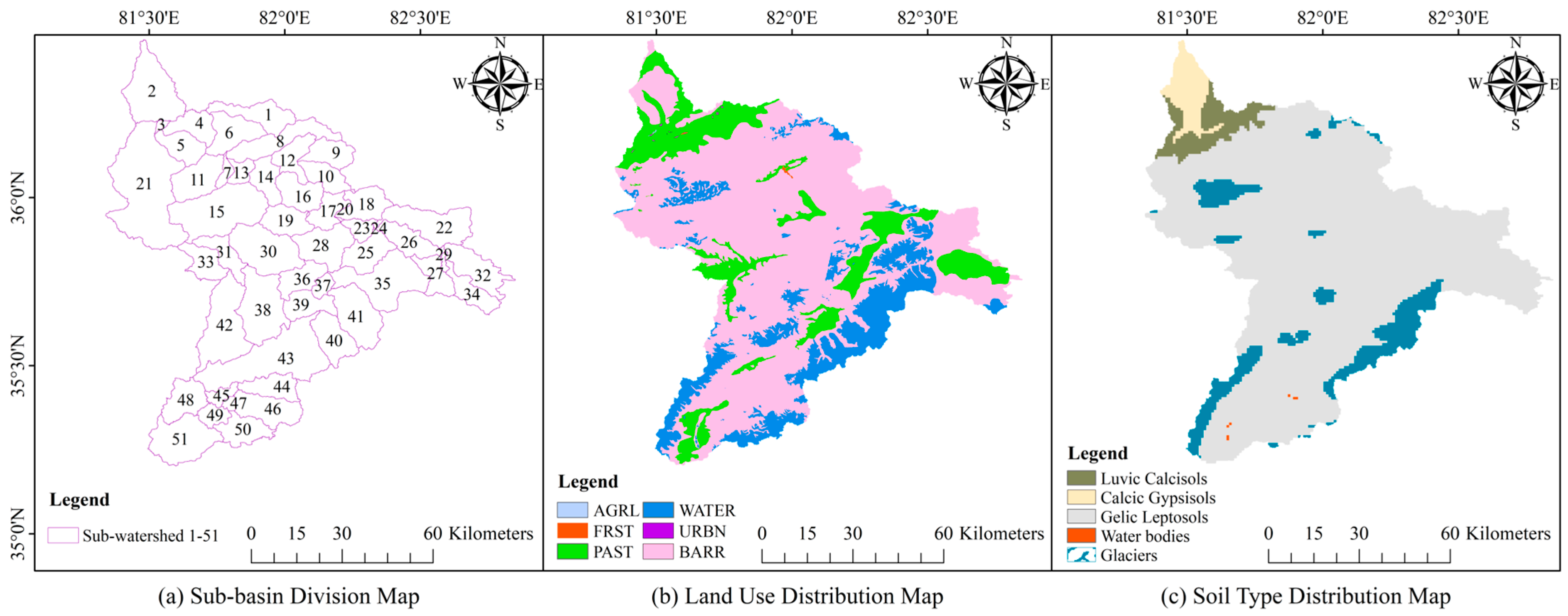
Using data from 1961 to 2015, the SWAT modeling framework was utilized to replicate the hydrologic process in the designated catchment. Utilizing a 30-m resolution DEM and land use data (categorized into 6 types), primarily unutilized land), and 1:1 million scale soil data, ArcSWAT 2012 divided the watershed into 51 sub-basins and 988 Hydrological Response Units (HRUs). Missing soil hydraulic parameters were calculated using SPAW software (version 6.02.75). The fundamental geospatial characteristics of the study area are depicted in Figure 3. Figure 3a shows the sub-basin delineation map, where 51 sub-basins are defined based on hydrological boundaries. These sub-basins extend in a dendritic pattern from high elevations to the middle and lower reaches, providing the spatial framework for model water balance calculations. Figure 3b displays the land use distribution map, color-coded for six land use types. It reveals that unutilized land dominates and is concentrated in the low-to-mid elevation zones, while high-elevation areas feature patchy grasslands and glaciers. This spatial heterogeneity directly influences hydrological processes such as evaporation and infiltration. Figure 3c presents the soil type distribution map, showing a clear “topography–climate” synergistic differentiation pattern: High-altitude cold zones develop highly permeable permafrost thin-layer soils, while arid-semiarid outlet areas form soil assemblages dominated by calcareous gypsum soils and clayified calcareous soils due to intense evaporation. This not only reveals the critical control of thermal-hydrological conditions on soil formation processes but also provides a crucial spatial foundation for accurately simulating runoff generation and infiltration processes. The three sub-maps comprehensively integrate key land surface attributes across the watershed, clearly revealing the interactive patterns of topography, land cover, and soil. This establishes a robust foundation for identifying hydrologically sensitive areas and simulating climate–hydrological responses.

Figure 3. Spatial Characteristics of the Kriya River Headwaters Region.

Model parameter calibration and validation were performed using the SUFI-2 algorithm within the SWAT-CUP (SWAT Calibration and Uncertainty Programs) software. Fourteen parameters were selected informed by the hydrometric characteristics observed at the Langan hydrological station. The time periods were defined as follows: 1961–1963 served as the model spin-up phase, 1964–1999 was designated for parameter estimation, and 2000–2015 was reserved for model validation. Through multiple iterations of the SUFI-2 algorithm, the optimal parameter set was obtained, as shown in Table 2. In the parameter modification scheme, the symbol “v” denotes the “assignment” operation (i.e., direct replacement of parameter values), while the symbol ‘r’ denotes the “multiply” operation (i.e., multiplicative adjustment of parameter values). The p-value indicates the degree of parameter sensitivity: a smaller p-value signifies greater influence of the parameter on calibration results, while a larger p-value indicates lesser influence. The absolute value of t represents the intensity of parameter sensitivity—a larger t value indicates stronger sensitivity, and a smaller t value indicates weaker sensitivity. t > 0 indicates that increasing the parameter leads to an increase in calibration results, t < 0 indicates that increasing the parameter leads to a decrease in calibration results.

Table 2. Key Parameters for SWAT Modeling.

Parameter	Physical Meaning	Initial Range	Adjustment Method	Optimal Value	p	t
SMFMX	Maximum snowmelt rate (mm/°C/day)	0~20	v	0.19	0.0000	11.6026
CN2	SCS runoff curve number	35~98	v	80.3	0.0000	5.0549
TIMP	Snow temperature lag coefficient	0~1	v	0.9	0.1751	−1.3612
SURLAG	Surface runoff lag time coefficient (days)	0.05~24	v	0.66	0.2509	1.1516
ESCO	Soil evaporation compensation factor	0~1	v	0.12	0.2881	−1.0654
ALPHA_BF	Baseflow recession coefficient	0~1	v	0.88	0.3073	−1.0238
EPCO	Plant transpiration compensation factor	0~1	v	0.83	0.3839	0.8727
CAMMX	Maximum canopy interception capacity (mm)	0~100	v	0.13	0.6171	−0.5009
GW_DELAY	Groundwater delay time (days)	0~500	v	391.7	0.7665	−0.2973
BIOMIX	Biological mixing efficiency	0~1	r	0.15	0.7739	−0.2877
SMFMN	Minimum snowmelt rate (mm/°C/day)	0~20	v	0.037	0.8491	−0.1904
TLAPS	Temperature lapse rate (°C/km)	−10~10	v	4.14	0.8618	0.1742
GW_REVAP	Groundwater revap coefficient	0.02~0.2	v	0.024	0.8900	0.1384
SMTMP	Base temperature for snowmelt (°C)	−20~20	v	1.57	0.9135	0.1088

The parameter results in Table 2 reflect the hydrological characteristics of cold and arid regions. Among them, the snowmelt parameters (SMFMX = 0.19, SMTMP = 1.57 °C) indicate a gradual glacier-snowmelt process, with the temperature decay rate confirming the terrain’s control over the temperature field. Among runoff parameters, the high SCS runoff curve number (CN2 = 80.3) aligns with the poor permeability of arid land surfaces. The small surface runoff lag coefficient (SURLAG = 0.66 days) indicates rapid runoff convergence, consistent with steep topography. Among groundwater parameters, the high baseflow decay coefficient (ALPHA_BF = 0.88) reflects slow decay, potentially linked to glacial recharge; the extended groundwater delay time (GW_DELAY = 391.7 days) reflects a slow recharge process. Sensitivity analysis results indicate that parameters such as SMFMX, CANMX, and SMTMP exhibit p-values below 0.05, classifying them as highly sensitive parameters with significant influence on simulation outcomes. However, the current model lacks a glacier module, imposing clear limitations in characterizing glacier ablation processes. This limitation partially affects the reliability of calibration results for relevant parameters (e.g., snowmelt-related parameters) and constrains the model’s simulation accuracy in glacier-fed catchments.

3.1.2. SWAT-LSTM Input Parameter Characteristics

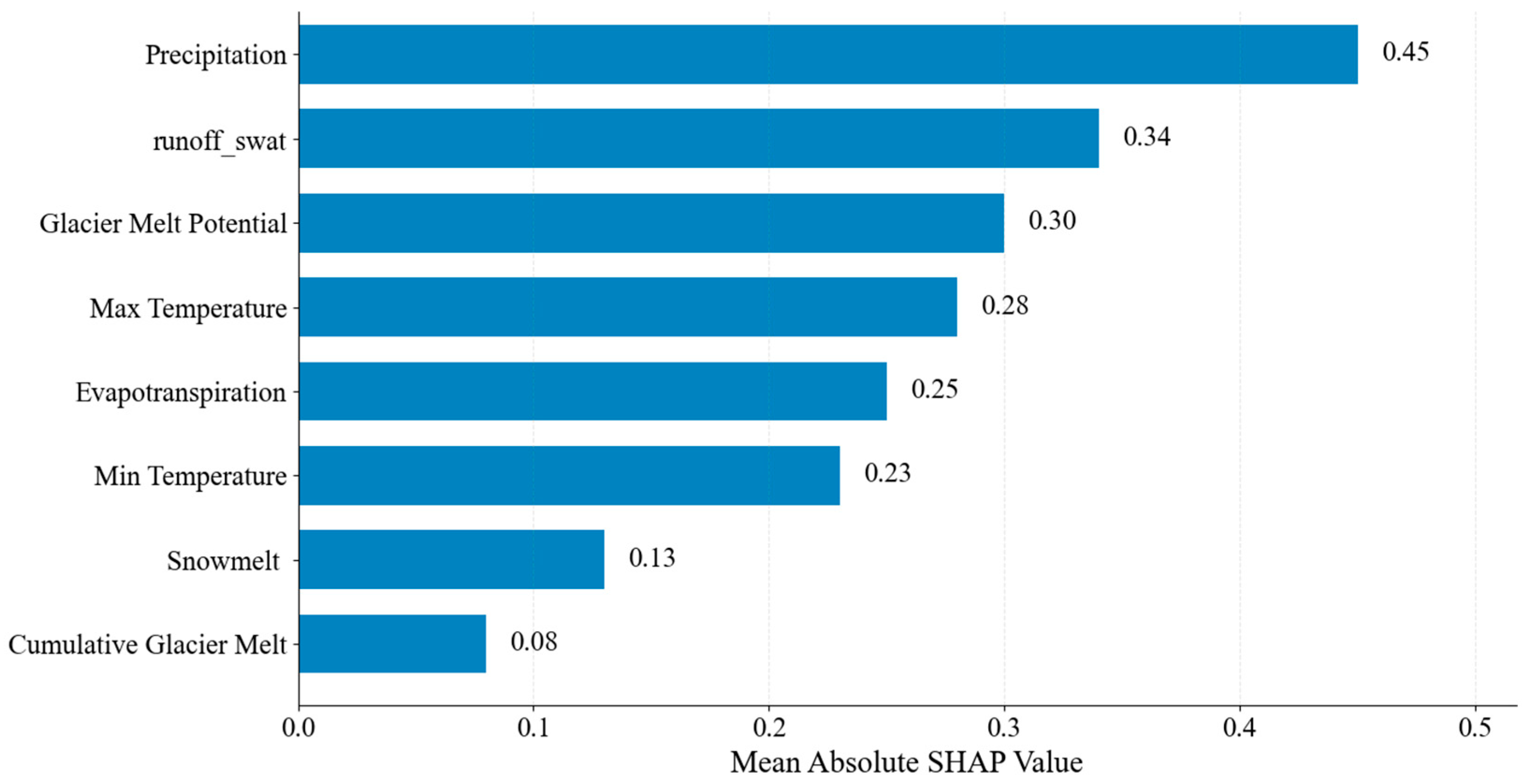
Figure 4 shows the ranking results of input parameter importance for the SWAT-LSTM coupled model. The results indicate that the contributions of various parameters to glacial meltwater runoff simulation vary significantly, revealing a clear hierarchy of driving factors. Among these, precipitation dominates with a SHAP value of 0.45, confirming its role as the most direct source of runoff in glacier-fed catchments and a key physical mechanism; SWAT simulated runoff (SHAP = 0.34) and glacier melt potential (SHAP = 0.30) ranked second and third, respectively, reflecting the LSTM model’s high dependence on the physical prior knowledge provided by the SWAT module. This also validates the effectiveness and innovation of introducing the glacier module in this study to address structural deficiencies in traditional hydrological models; Among the temperature factors, both maximum temperature (SHAP = 0.28) and minimum temperature (SHAP = 0.23) exhibited significant influence, reflecting the fundamental role of temperature in driving the ice and snow melt process. The slightly higher contribution of maximum temperature may be related to the strong energy input during the daytime; Additionally, evapotranspiration (SHAP = 0.25) and snowmelt runoff (SHAP = 0.13) also provided distinct yet relatively minor contributions to the simulation results, indicating that the model simultaneously accounts for both water dissipation processes and seasonal snowpack effects; The contribution of cumulative glacier melt (SHAP = 0.08) is relatively low, possibly due to information overlap with other glacier characteristics. Nevertheless, it demonstrates the model’s ability to capture the long-term memory effect in glacier mass balance.

Figure 4. Importance Ranking of Input Parameters for the SWAT-LSTM Coupled Model.

3.1.3. Runoff Simulation Based on the SWAT and SWAT-LSTM

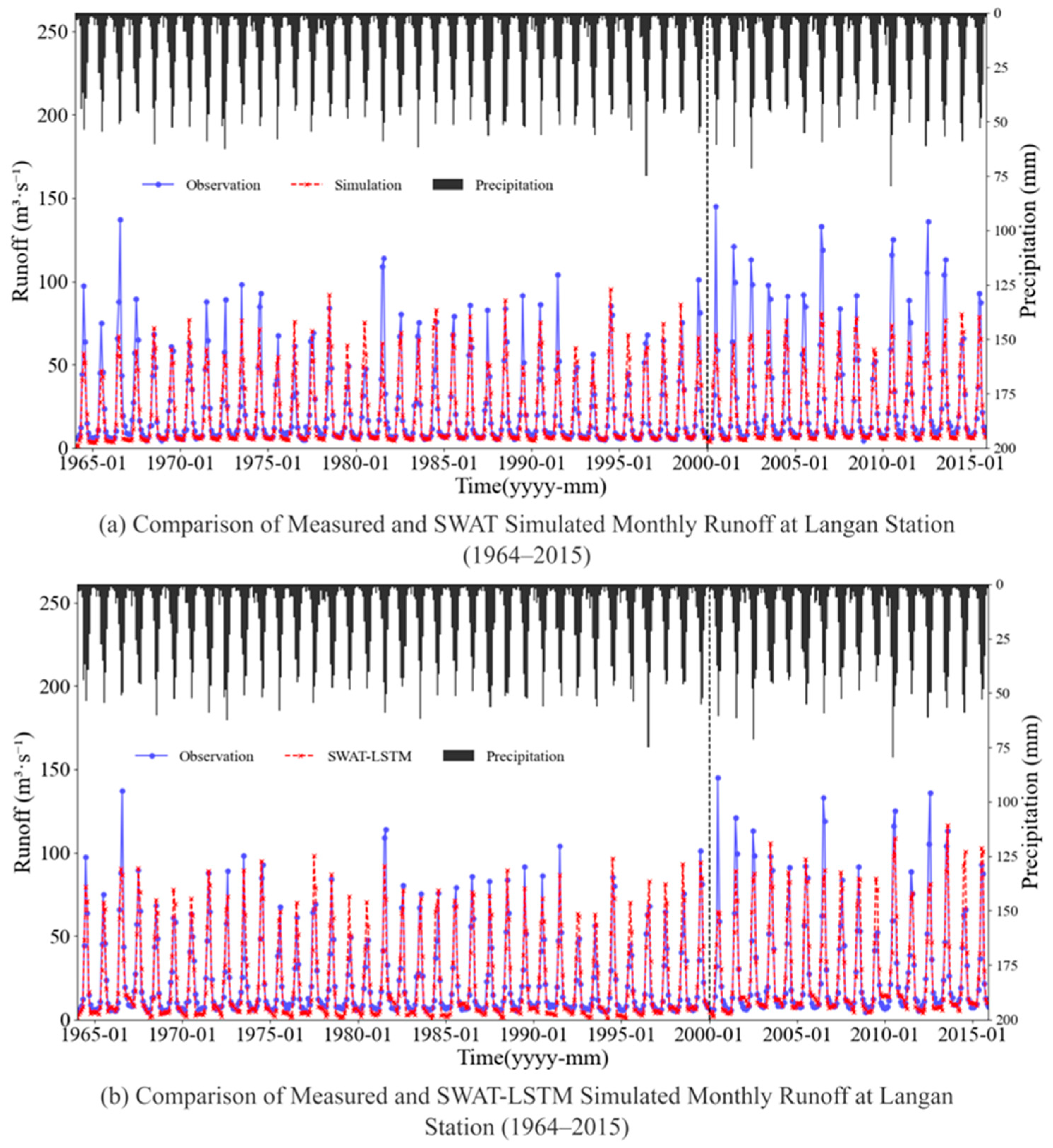
Figure 5 shows the runoff simulation results from SWAT and SWAT-LSTM. The models employed a warm-up period from 1961 to 1963, which was excluded from the simulation process; thus, the study period commenced in 1964. Given that the Jiyin Reservoir construction commenced upstream of the hydrological station in 2016, to avoid human activity impacts, this simulation selected natural runoff modeling prior to reservoir construction, with the study period ending in 2015. Thus, the study period in Figure 4 is defined as 1964–2015, encompassing the calibration period (1964–1999) and the validation period (2000–2015). The SWAT model simulation results for the upper reaches of the Keriya River are shown in Figure 5a. During the calibration period (1964–1999), the model demonstrated excellent performance (R² = 0.775, NSE = 0.777, PBIAS = 4.52%), accurately capturing both runoff trends and total runoff volume. During the validation period (2000–2015), although trend consistency remained robust (R² = 0.805, NSE = 0.735), a significant systematic bias emerged (PBIAS = 19.75%), with simulated total runoff values substantially lower than observed values. This discrepancy reflects the structural limitations of the SWAT model in basins dominated by glacial meltwater recharge, as its lack of a glacier module makes it difficult to accurately capture the contribution of glacial melt to runoff. To enhance the model’s generalization capability, a SWAT-LSTM hybrid model was developed. The simulated runoff values exhibited significantly better agreement with observed data compared to the former model, as shown in Figure 5b.

Figure 5. Comparison of observed monthly runoff at Langan Station and SWAT/SWAT-LSTM simulated values (1964–2015).

The comparison results of the hydrological simulation performance between the SWAT model and the SWAT-LSTM hybrid model for the Keriya River headwaters region are shown in Table 3. At the calibration period (1964–1999), the NSE and R² of the SWAT-LSTM hybrid model were 0.869 and 0.885, respectively, which were higher than the 0.775 and 0.777 of the SWAT model, increasing by 12.1% and 13.9%, respectively. The PBIAS decreased from 4.52% of the SWAT model to 0.17%, indicating that the system bias was significantly reduced. During the verification period (2000–2015), the NSE and R² of SWAT-LSTM were 0.847 and 0.847, respectively, which were better than 0.735 and 0.805 of SWAT model, and the NSE attenuation rate was only 2.5%, which was lower than 5.2% of SWAT model, indicating that SWAT-LSTM had strong generalization ability and stability. From the perspective of error indicators, the RMSE and MAE of SWAT-LSTM are 8.80 m³/s and 5.89 m³/s, respectively, which are 23.5% and 6.4% lower than those of SWAT model. The RMSE and MAE in the validation period were 12.78 m³/s and 7.56 m³/s, respectively, with a decrease of 23.8% and 18.4%, respectively, indicating that it had better performance in high flow events and average deviation control. The SWAT-LSTM model effectively integrates physical process constraints with the nonlinear temporal feature capture capability of deep learning. Compared to similar studies in cold and arid regions—such as the pure SWAT model in the Zamu River basin (NSE = 0.73, PBIAS > 10%) and the multi-source meteorological data-driven model in the Shiyang River basin (NSE 0.50–0.76), achieving a performance improvement exceeding 99% reduction in bias [53,54]. Its advantage lies in the SWAT module establishing physical plausibility, thereby avoiding paradoxes that may arise in pure LSTM models. Meanwhile, LSTM effectively corrects the systematic bias in SWAT through residual learning (reducing PBIAS from 19.75% to 0.06%). SWAT-LSTM achieves significant improvements in both accuracy and robustness, offering a novel approach that integrates mechanistic strengths with data advantages for hydrological modeling in cold, arid regions.

Table 3. Comparison of Evaluation Metrics Between SWAT and SWAT-LSTM Models.

Model	The Calibration Period (1964–1999)					The Verification Period (2000–2015)
	NSE	R2	PBIAS	RMSE (m3/s)	MAE (m3/s)	NSE	R2	PBIAS	RMSE (m3/s)	MAE (m3/s)
SWAT	0.775	0.777	4.52%	11.51	6.29	0.735	0.805	19.75%	16.78	9.27
SWAT-LSTM	0.869	0.885	0.17%	8.80	5.89	0.847	0.847	0.06%	12.78	7.56

3.2. Comparison Analysis of Actual Runoff and Natural Runoff Restoration After Reservoir Construction

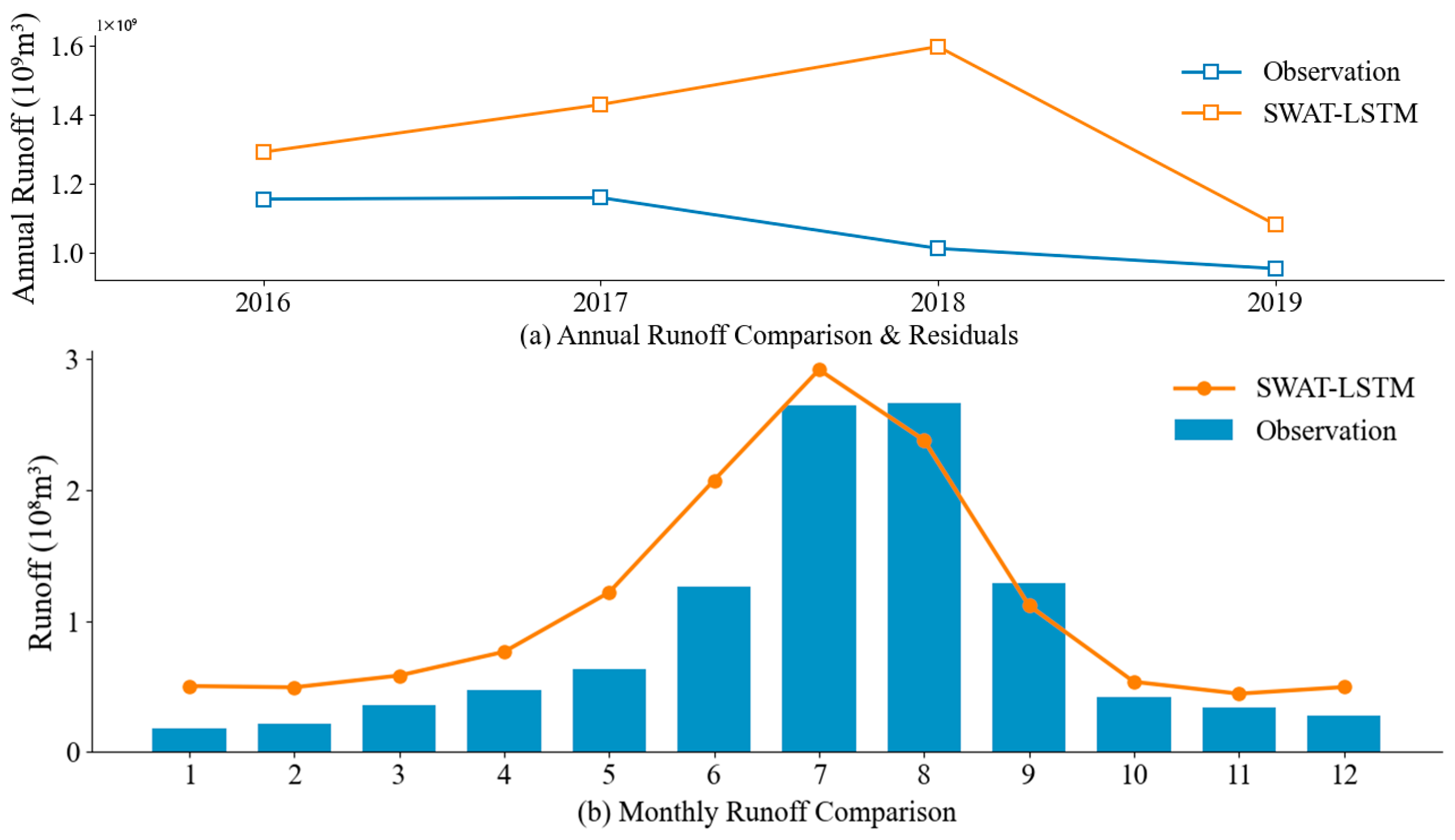
To investigate the comparison between actual runoff and natural runoff after the completion of Jiyin Reservoir, the study period was set to begin in 2016, as the reservoir began impoundment that year. Since the available runoff data only extends through 2019, the study period for Figure 6 was defined as 2016–2019. A comparative analysis based on natural runoff reduction results (Figure 6a) reveals that observed annual runoff exhibits a continuous decline trend, whereas SWAT-LSTM model simulations show an initial increase followed by a decrease during the same period. The discrepancy was particularly pronounced in 2018: simulated runoff reached 1.60 × 10⁹ m³, whereas observed values recorded only 1.01 × 10⁹ m³, representing a 58.4% difference. The coefficient of variation for the observed sequence was 16.7% lower than that of the simulated values, reflecting the reservoir’s typical regulation function of “cutting peaks and filling valleys.” This smoothed the intra-annual and interannual fluctuations of natural runoff, consistent with the core function of reservoirs in arid regions to optimize water resource allocation [55]. In 2019, simulated values decreased by 32.3%, yet observed values remained 11.8% lower than simulated values. Multi-year monthly averages (Figure 6b) further reveal that the model-simulated natural runoff peaked significantly higher than observed values in June–July, with a peak difference of approximately 43%, visually confirming the reservoir’s flood storage effect during the flood season. However, observed runoff (blue bar chart) in August–September exceeded SWAT-LSTM model simulations (orange line chart). This “anomalous” high value likely stems from human intervention: downstream reservoirs released water based on actual demand (e.g., agricultural irrigation), increasing non-flood season discharge volumes [56].

Figure 6. Comparison of Runoff Simulation Results at Langan Hydrological Station After Reservoir Construction: Annual Scale and Monthly-Scale SWAT-LSTM Performance Evaluation (2016–2019).

3.3. Verification of Glacier Area Dynamics and Runoff Hydrological Response Mechanisms

3.3.1. Validation and Analysis of Glacier Area Dynamics

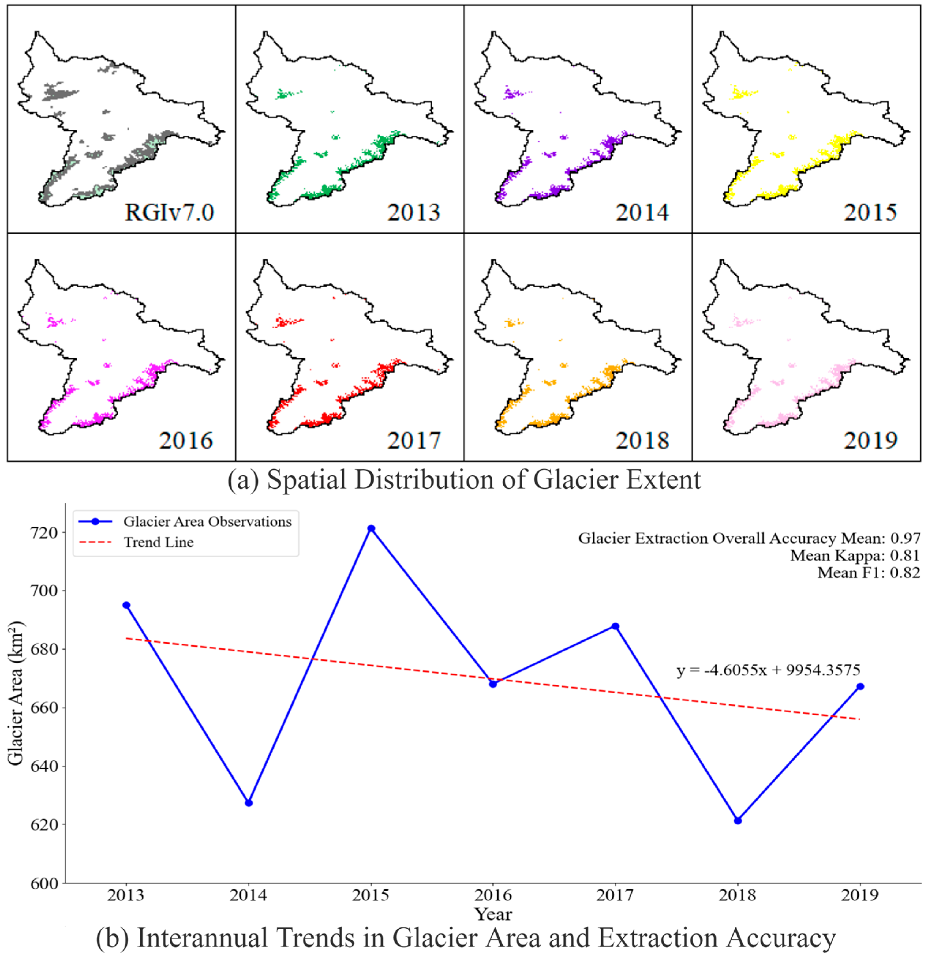
The study selected the period from 2013 to 2019 for glacier change analysis and conducted spatial comparison validation based on high-resolution remote sensing extraction results and RGI v7.0 benchmark data (Figure 7). Given that the scan line corrector for Landsat 7 imagery malfunctioned after 2003, resulting in inconsistent data quality, its extraction accuracy remains lower than Landsat 8 even when employing identical extraction methods. Therefore, Landsat 7 imagery was excluded from this study. Landsat 8 imagery, however, has been continuously available since 2013, providing stable 30-m high-resolution data support for glacier identification. Consequently, the glacier validation period was set to commence in 2013. Since the runoff data obtained for this study ended in 2019, the final validation period was determined to be 2013–2019. However, the hydrological model validation period spans 2000–2015. If the glacier validation period also ended in 2015, the time span would be only three years (2013, 2014, and 2015). Such a short period would render the analysis unrepresentative. Therefore, earlier data were not included in the unified analysis process. This also resulted in the glacier validation period and the hydrological model validation period not fully overlapping in time.

Figure 7. Spatial–Temporal Variations and Accuracy Validation of Glaciers in the Upper Kriya River Basin (2013–2019).

Figure 7a illustrates changes in glacier spatial distribution from 2013 to 2019, revealing that glaciers are primarily concentrated in high-altitude areas and maintain relatively stable spatial distribution patterns across years. Change detection results indicate that glaciers exhibited overall continuous retreat during the study period, manifesting in two typical degradation patterns: first, significant retreat of glacier terminals, particularly pronounced in lower-elevation ice tongues; second, accelerated fragmentation of glacier areas, with previously contiguous glaciers progressively splitting into multiple smaller ice bodies. Figure 7b illustrates that the glacier area fluctuated between 627 and 720 km², with an average annual retreat rate of 4.61 km²/a. From an accuracy assessment perspective, this further validates the reliability of the extraction results. The average overall accuracy reached 0.97, with a Kappa coefficient of 0.81 and an F1 score of 0.82, indicating high consistency in the applied method for glacier boundary identification. Notably, glacier area exhibited fluctuations between 2013 and 2019, potentially influenced by cloud cover during image acquisition or extreme weather events. Nevertheless, the sustained retreat trend observed throughout this period provides crucial spatial data for understanding the impact of glacial changes on runoff.

3.3.2. Validation of Glacier–Runoff Hydrological Response

Based on a systematic assessment of the glacier–runoff hydrological response relationship, the SWAT-LSTM coupled model exhibits unique simulation characteristics. From the perspective of statistical significance, the glacier–runoff correlation coefficient analysis presented in Figure 8 reveals a key contradiction: although the SWAT-LSTM coupled model failed to achieve statistically significant correlation coefficients both globally (Figure 8a: r = −0.159) and during the ablation season (Figure 8b: r = −0.129), its numerical direction aligns more closely with the expected physical mechanisms. The lack of statistical significance may stem from the limited availability of glacier change monitoring data during the study period (2013–2019), resulting in insufficient sample size for conventional significance testing.

Figure 8. Comparison of Correlation Coefficients Between Glacier Area Change and Runoff Simulation.

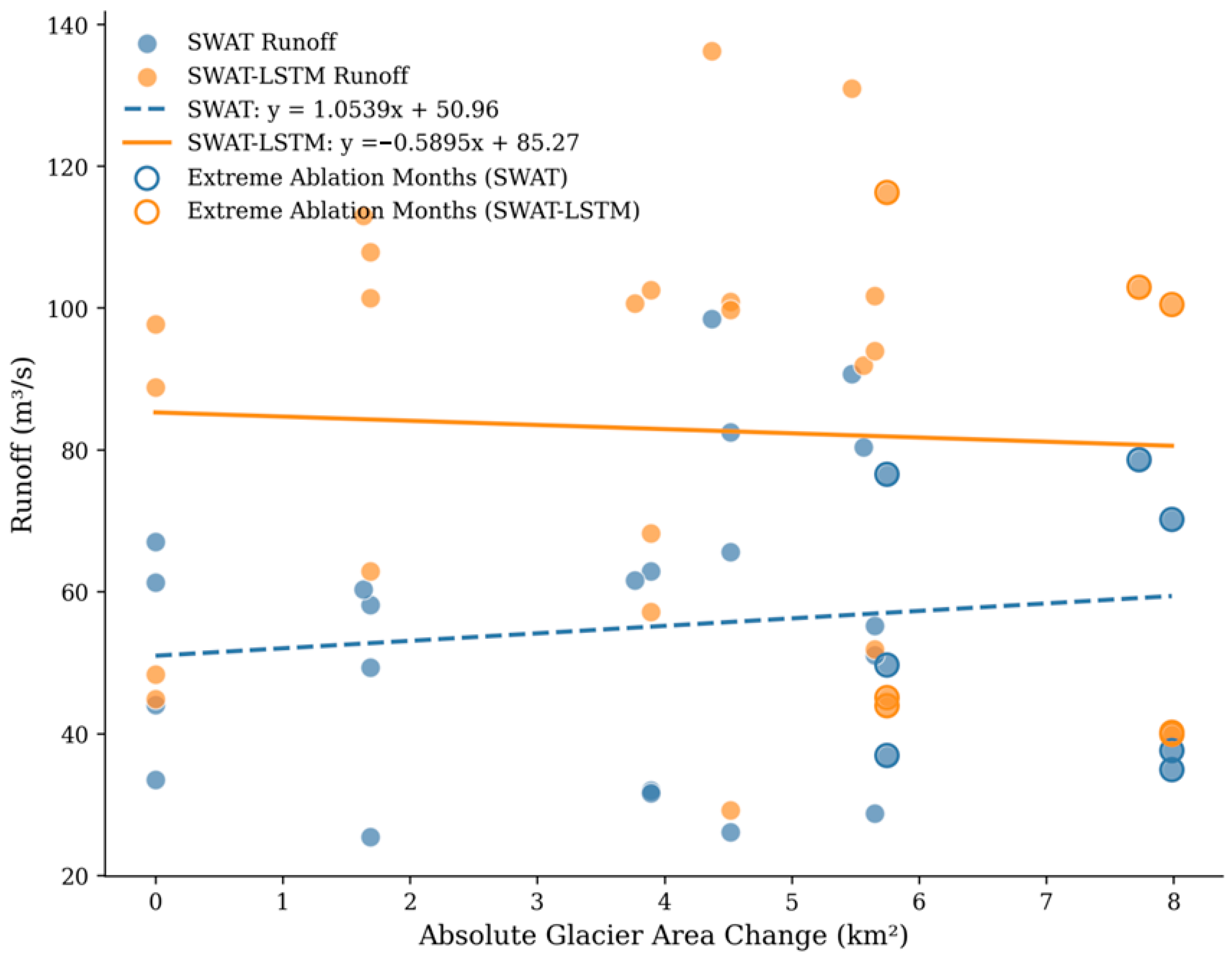
The regression analysis in Figure 9 provides further evidence supporting the physical mechanism. The ablation season regression slope in SWAT-LSTM undergoes a fundamental shift, reversing from the positive slope (+1.0539) in the SWAT model to a negative slope (−0.5895). This change aligns strongly with the physical mechanism that “increased glacier ablation leads to elevated short-term runoff” [57]. Although both models exhibit low R² values, reflecting the complexity of the glacier–runoff relationship, the reversal of slope signs carries significant physical implications. At the physical mechanism level, the study identified a key phenomenon: during extreme ablation months, SWAT-LSTM simulated runoff values averaged 27.1% higher than those from the SWAT model. This near-significant improvement indicates that the coupled model, by integrating the glacier module, more accurately captures the hydrological response to high-intensity ablation events, reflecting the negative feedback mechanism between glacier ablation and runoff. However, the absence of delayed responses (such as groundwater recharge lags) may be related to glacier thickness, highlighting the need for models to balance transient and long-term response processes.

Figure 9. Relationship between Glacier Melt Volume and Runoff Response During the Melting Season (June–September).

A comprehensive analysis of Figure 8 and Figure 9 reveals that the core advantage of the SWAT-LSTM model lies in its enhanced physical mechanism rationality, particularly demonstrating improved potential in simulating extreme climate events. Future efforts should focus on extending glacier observation sequences, integrating remote sensing data on glacier thickness, and developing a lag module that accounts for glacier dynamics. These measures will further enhance the model’s statistical significance and mechanistic representation capabilities in simulating hydrology in cold regions.

3.4. CMIP6 Model Simulations of Climate Change in the Study Area CMIP6 Models Simulate Climate Change in the Study Area

3.4.1. Downscaling and Bias Correction Results

The Taylor plot was used to evaluate the simulation capabilities of CMIP6 models, with results shown in Figure 10. The selection of 1975–2014 as the simulation period is primarily based on its coverage of a relatively complete climate observation sequence, while also considering the availability and consistency of CMIP6 model data. This facilitates the assessment of models’ ability to capture regional climate characteristics within a long-term context. Although downscaled GCM models exhibit differences in simulating climate conditions in the source region of the Kriya River basin, all models effectively capture the historical trends in monthly mean temperature and precipitation. Compared to individual models, the Multi-Model Ensemble (MME) outperformed any single model. Its correlation coefficients with observed data reached 0.93 for monthly precipitation (Figure 10a), 0.95 for daily minimum temperature (Figure 10b), and 0.92 for daily maximum temperature (Figure 10c). This result indicates that the MME method can effectively reduce structural uncertainty in single-mode systems, consistent with recent research findings [58].

Figure 10. Taylor diagram assessment of CMIP6 and MME models in the Kriya River headwaters region (1975–2014).

This study employs a multi-temporal analysis strategy to align with the data requirements and research objectives of different problems. The analyses depicted in the figures above are based on historical data, with temporal ranges varying according to data availability. Examples include model results (Figure 5), human activity impacts (Figure 6), glacier dynamics (Figure 7), and climate model validation (Figure 10). However, all analyses adhere to a unified methodological framework—such as SWAT-LSTM coupling and CMIP6 downscaling—ensuring comparability of results and overall scientific rigor.

3.4.2. Future Climate Change

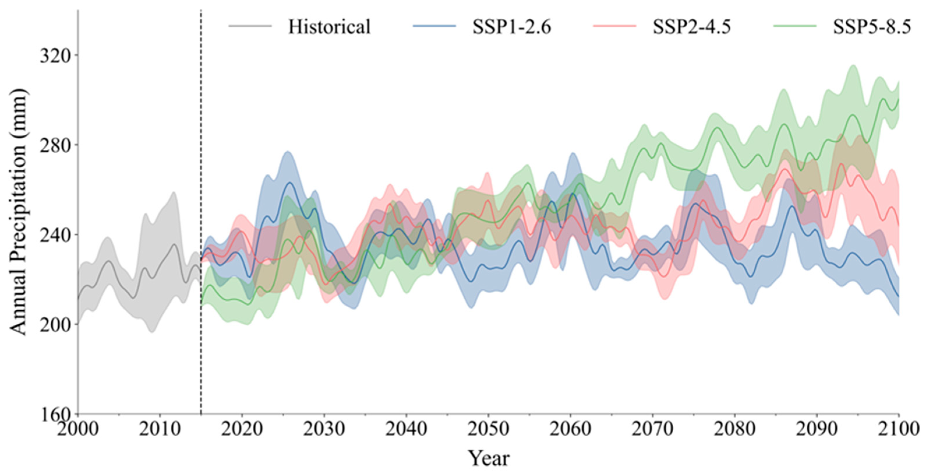
Based on the historical reference period from 2000 to 2015, this study compares and analyzes the future precipitation change characteristics across Chinese regions under different climate scenarios. Results show (Figure 11) that under the low-carbon pathway SSP1-2.6 scenario, precipitation increments in the 21st century exhibit a pattern of “mid-term > long-term > near-term.” with increases of 4.94%, 5.76%, and 5.16% relative to the baseline period during the 2026–2050, 2051–2075, and 2076–2100 periods, respectively, representing an overall increase of approximately 5%. Under the medium pathway SSP2-4.5 scenario, precipitation increases escalate in a stepwise pattern: rising from 7.45% in the near-future to 8.06% by mid-century, and significantly increasing to 13.62% by the end of the century. The high-carbon SSP5-8.5 pathway exhibits markedly nonlinear growth, with the increase surging from 5.23% in the near term to 16.43% in the mid-term, and further reaching 26.83% by 2100—representing a progressive rise of 21.60%. Comparisons across three scenarios reveal a pronounced positive correlation between precipitation changes and radiative forcing intensity. Particularly during 2076–2100, precipitation increases under the SSP5-8.5 scenario could reach 5.2 times those under the SSP1-2.6 scenario, highlighting the critical influence of carbon emission pathways on regional water cycles. This precipitation pattern aligns with the IPCC AR6 report’s conclusion of “intensified wet-dry differences” in global precipitation, indicating that under high-emission scenarios, regional water cycles intensify while spatial heterogeneity becomes pronounced [59].

Figure 11. Annual Precipitation in the Upper Kriya River Basin (2000–2100).

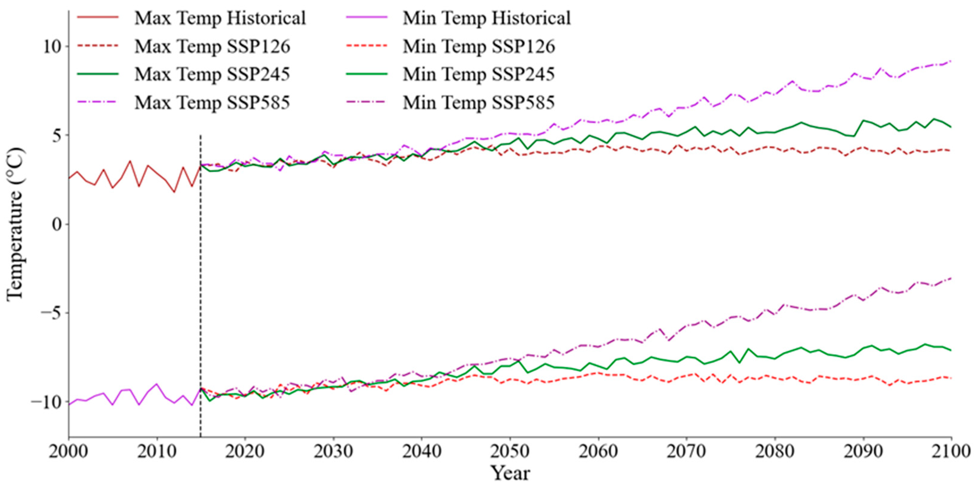
Simulations based on Shared Socioeconomic Pathways (SSPs) reveal significant variations in temperature responses across different emission scenarios within the Kriya River headwater catchment (Figure 12). Under the low-emission SSP1-2.6 pathway, the maximum temperature increase exhibits a “slow rise-stabilization” trend between 2000 and 2100, with three-stage warming increments of 1.14 °C, 1.51 °C, and 1.48 °C, respectively. The minimum temperature increase stabilizes below 1 °C after 2050. Under the medium-emission scenario SSP2-4.5, maximum temperatures accelerated their rise in the latter half of the century (0.04 °C/decade), reaching 2.75 °C by 2100 (range 2.28–3.26 °C), while minimum temperatures concurrently increased to 2.53 °C. The high radiative forcing scenario (SSP5-8.5) leads to abrupt warming, with maximum temperatures rising by 5.39 °C (range 4.21–6.53 °C) by century-end and minimum temperature extremes exceeding 6.67 °C. The study found that under SSP5-8.5, the increase in maximum temperatures between 2076 and 2100 is 3.6 times greater than under SSP1-2.6, while the interannual variability expands by 5.6 times [60].

Figure 12. Temperature Variation in the Kriya River Headwaters Region (2000–2100).

3.5. Annual Runoff Variations Under Future Climate Change Scenarios Based on SWAT-LSTM

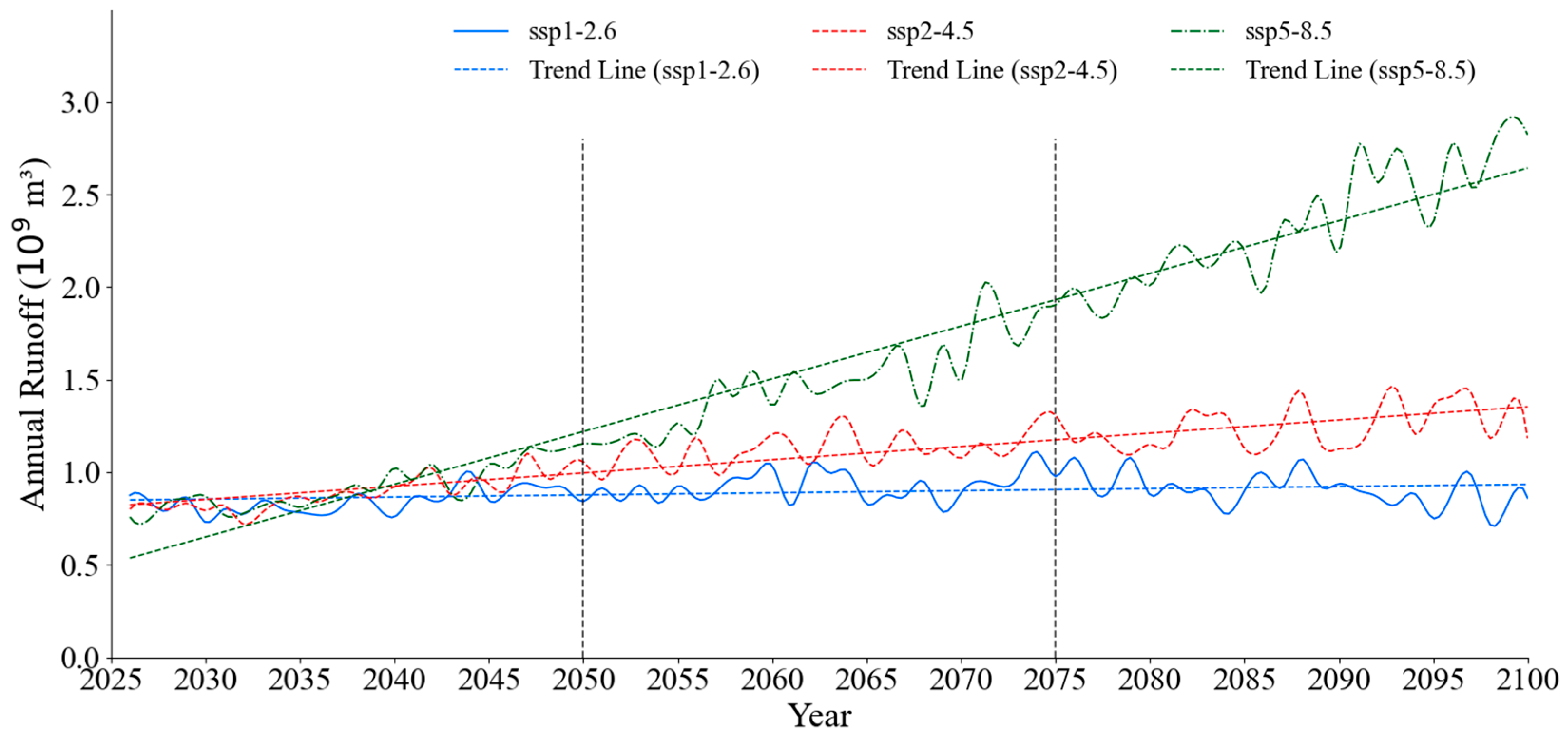
Projected annual runoff in the upper Kriya River under SSP1-2.6, SSP2-4.5, and SSP5-8.5 scenarios throughout 2026–2100 is presented in Figure 13. As shown, the annual runoff at the Langan hydrological station exhibits no significant increase within the SSP1-2.6 framework, a slight increase under SSP2-4.5, and a markedly pronounced upward trend under SSP5-8.5.

Figure 13. Simulated Annual Runoff Values at the Outflow of Langan Hydrological Station Under Three Scenarios (2026–2100).

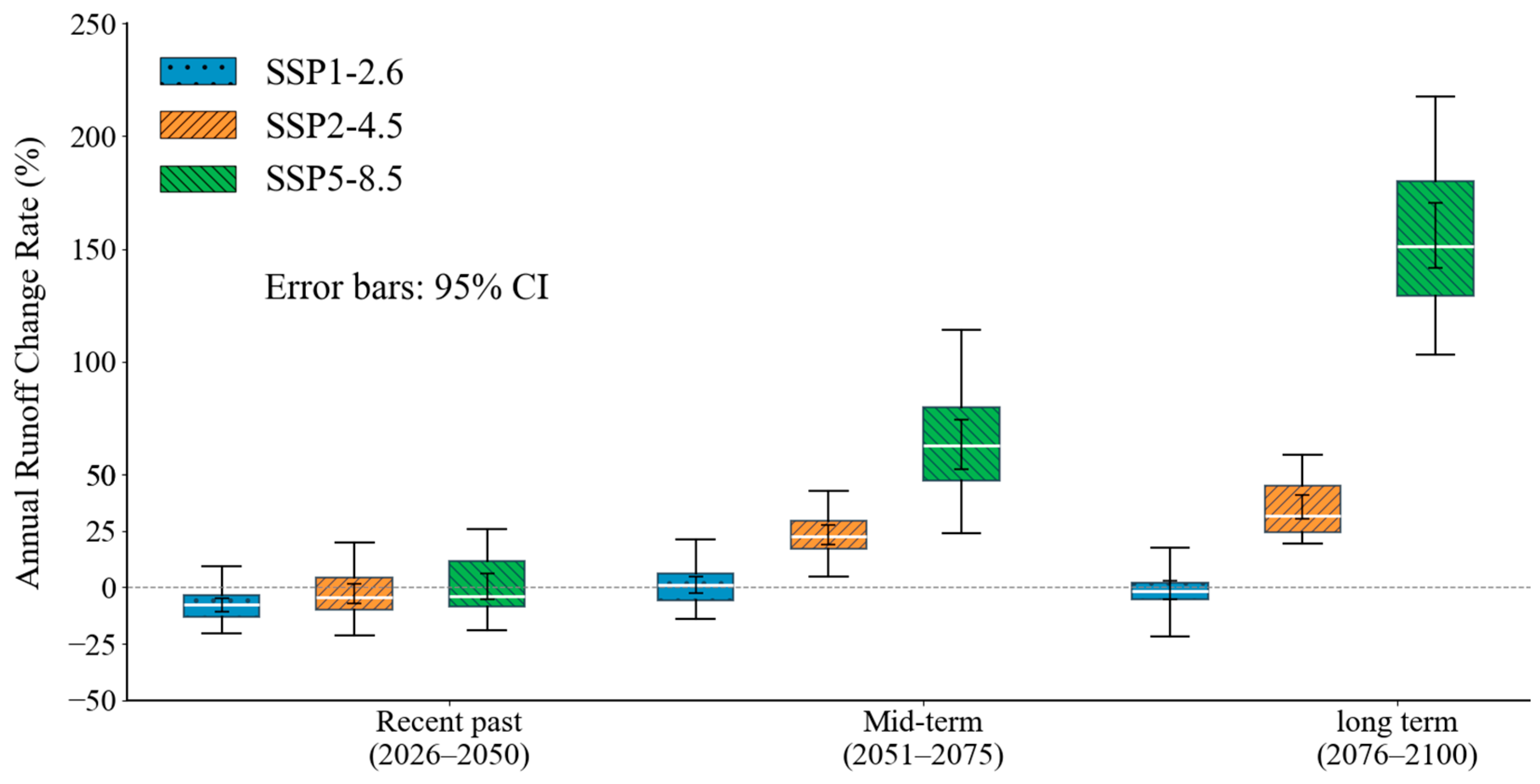
Figure 14 shows the distribution of annual average runoff change rate and its 95% confidence interval under different shared socioeconomic paths (SSP1-2.6, SSP2-4.5, SSP5-8.5) in the source region of the Keriya River in the near term (2026–2050), medium term (2051–2075), and long term (2076–2100). The box plot and error line jointly reveal the evolution characteristics and uncertainty range of runoff response under different climate scenarios. In the near term, the runoff change rates under the three scenarios are relatively flat. The mean values of SSP1-2.6, SSP2-4.5 and SSP5-8.5 are −7.90%, −2.77% and 0.41%, respectively, and their confidence intervals are −10.78%~−5.03%, −6.99%~1.44% and −5.25%~6.07%, respectively. Some intervals span zero values, indicating that there is a certain uncertainty in the direction of runoff change in the short term. The shape of the box shows that SSP1-2.6 is left-skewed (Q1 = −13.16%, median = −7.73%, Q3 = −3.66%), reflecting a higher possibility of runoff reduction. The right end of the box of SSP5-8.5 extends to 25.84%, and Q3 reaches 11.44%, suggesting an increasing trend in runoff under this scenario. In the mid-term, the difference between scenarios expanded significantly. The runoff under the SSP2-4.5 and SSP5-8.5 scenarios increased significantly, with the mean values rising to 23.34% and 63.58%, respectively, and the confidence intervals were 19.18–27.50% and 52.61–74.55%, respectively, which did not cross the zero value, indicating that the results had high statistical reliability. The upper limit of the SSP5-8.5 box is 114.34%, and the Q3 is 79.96%, indicating that there is a large increase in some simulation results and obvious right deviation characteristics. In the long term, the runoff change rate under the SSP5-8.5 scenario increased sharply, with a mean value of 156.20%, a confidence interval of 141.84–170.56%, a box upper limit of 217.81%, a Q3 of 180.08%, and a median of 151.30%, further confirming the extreme increase trend of runoff under the high emission path. In contrast, the runoff changes in the SSP1-2.6 scenario remain at a low level (mean value is −1.29%), the box range is between −21.66% and 17.74%, and the confidence interval covers zero values, reflecting that the direction of its change is still uncertain. Overall, Figure 14 illustrates the evolution paths of downslope flow variations under different climate scenarios and the associated uncertainties. In the high emission scenario (SSP5-8.5), the downflow increases significantly and the uncertainty increases with the extension of the period, while in the low emission scenario (SSP1-2.6), the downflow changes more gently, but the uncertainty persists. The results highlight the importance of mitigation measures to mitigate future runoff fluctuations and reduce hydrological risks.

Figure 14. Interannual Variability of Simulated Annual Runoff at the Outflow of Langan Hydrological Station Under Three Scenarios (2026–2100) (Note: Box boundaries represent the 15th and 75th percentiles; the horizontal line within the box indicates the median; upper and lower limits denote the maximum and minimum values).

The variation in future runoff scenarios primarily stems from the nonlinear impact of rising temperatures on glacial melt. The projected 151.30% surge in runoff by the end of the century under a high radiative forcing future (SSP5-8.5) is likely closely linked to accelerated glacial melt under high-emission pathways [61]. However, the wide range of projected runoff values—such as the long-term range of 103.18% to 217.81% under SSP5-8.5—highlights significant uncertainties stemming from CMIP6 model variability, downscaling biases, and glacier module parameterization (e.g., simplified ice thickness dynamics may overestimate long-term meltwater contributions) [62,63]. From a water resources management perspective, while the steep increase in runoff under the SSP5-8.5 pathway may yield short-term surpluses, the subsequent depletion of glacial reserves will trigger profound water crises. This necessitates forward-looking basin planning to address the risk of abrupt runoff changes under high-emission scenarios. Enhancing the sustainability and resilience of water systems requires improving the characterization of glacial mass balance and developing adaptive management strategies.

3.6. Limitations and Future Research Directions

This study achieved satisfactory simulation performance using the SWAT-LSTM coupled model in the Kriya River headwaters, yet several limitations remain. Regarding data and physical process characterization, the model heavily relies on high-quality input data (e.g., soil properties, long-term meteorological–runoff observations), posing challenges for transfer applications to data-scarce basins. Significant weaknesses exist in glacier mass balance characterization: Landsat 8’s 30-m resolution underestimates glacier area by approximately 12% in steep slope areas [64], and the contribution of ice thickness changes to meltwater has not been quantified [65]. Statistical results indicate that the glacier–runoff response relationship fails to reach significance (r = −0.129, p = 0.513), reflecting the model’s limited ability to capture complex glacier ablation processes. In terms of human activities and uncertainty propagation, in order to give priority to clarifying the independent driving effects of climate change, this study sets the underlying surface conditions and human activities (such as reservoir operation) as a constant background in future scenario prediction. Although this ‘ scenario isolation ‘ method helps to establish the baseline of climate response, it also leads to the inability of the model to achieve accurate and comprehensive prediction in the strong expectation of future human activities (such as reservoir operation and land conducive change) [66]. Sensitivity in glacier parameters (e.g., degree-day factors) within the SWAT module increases result uncertainty, which propagates through the coupling framework to the LSTM module. Uncertainties in climate change projections (emission scenarios, GCM structural differences, internal variability) propagate through the “GCM → downscaling → SWAT-LSTM” chain, resulting in excessively broad runoff prediction ranges [67]. Additionally, the model exhibits issues such as strong regional parameter dependence, LSTM black-box characteristics, lack of sensitivity analysis, and inadequate representation of hydrogeological processes [28].

To address these limitations, future research should develop a comprehensive improvement framework: enhancing model transferability in data-scarce regions through transfer learning strategies [14], employing synergistic multi-platform satellite data (e.g., Sentinel-1/2, ICESat-2) and coupling with ice dynamics models to enhance glacier mass balance characterization [66]. It is particularly critical to develop a reservoir operation rule generator based on deep reinforcement learning [68], and build a dynamic land use change scenario. Finally, a comprehensive prediction framework of ‘climate scenario–land use scenario–water resources management scenario’ is realized to provide a more comprehensive picture of water resources evolution. By introducing Bayesian deep learning frameworks to unravel parameter error propagation mechanisms and integrating diverse methodologies—including ensemble modeling, SUFI-2 uncertainty quantification, parameter regionalization, explainable AI, global sensitivity analysis, and groundwater coupling simulations [69,70,71,72], systematically enhancing model robustness and transparency. These integrated improvement strategies collectively advance cold-arid region hydrological modeling from a singular simulation tool toward a reliable decision support system, providing a more robust scientific foundation for adaptive water resource management.

4. Conclusions

This study established a SWAT-LSTM modeling paradigm featuring a ternary coupling of “physical mechanisms–deep learning–Glacier Module” tripartite coupling SWAT-LSTM modeling paradigm. By integrating SWAT’s physical constraints, LSTM’s nonlinear temporal feature capture capability, and basin glacier dynamics data, this approach overcomes the structural limitations of traditional models in characterizing glacier ablation processes. It significantly enhances hydrological simulation accuracy in high-altitude glacier-fed basins (validation period NSE reaches 0.847, PBIAS reduced to 0.06%, with errors decreased by over 99%). This provides a transferable, high-precision simulation solution for glacier-fed watersheds, offering novel and original contributions to the field of hydrology.

The study deepens the understanding of the multi-process coupling driving mechanism of ‘climate–cryosphere–human activities’ under climate change. Based on the downscaling analysis of CMIP6 multi-model ensembles, the nonlinear feedback relationship of climate–hydrological processes under different SSP scenarios is revealed, and the amplification effect of carbon emission path on hydrological extreme events is highlighted, and the reservoir regulation effect is quantified. In response to the challenges of climate change, it provides important theoretical support for hydrological modeling in data scarcity and high-altitude areas.

This study provides three suggestions for local water management departments and policy makers. First, establish a dynamic scheduling mechanism driven by climate scenarios in the Jiyin Reservoir, use the SWAT-LSTM model to predict runoff, and implement ‘impounding before flood season and replenishing during dry season’ to ensure ecological base flow. Secondly, the extreme value early warning system of meteorological–hydrological coupling is constructed, and the flood and drought event prediction is realized based on CMIP6 multi-model to reduce disaster risk. Thirdly, the red line management of ecological water use is strictly controlled, and the minimum ecological flow of glaciers to rivers is determined according to the actual situation of glacier retreat, so as to ensure the sustainability of oasis water use.

The construction of the SWAT-LSTM coupling framework provides a useful attempt for the hydrological model from a single mechanism-driven to a combination of physical mechanism and data-driven modeling ideas. This method shows good adaptability in inland river basins in high-altitude cold and arid regions where data are relatively scarce, and provides a theoretical basis and decision support for sustainable management of water resources under the background of climate change.

Future research should focus on key directions to improve model universality and decision support. The first is to integrate multi-source remote sensing data and coupling ice dynamics models to accurately characterize glacier mass balance. The second is to strengthen the quantification of the coupling mechanism of human activities, develop a deep reinforcement learning generator, and embed human water intake into the SWAT-LSTM model chain to reduce simulation bias. Thirdly, the Bayesian deep learning framework and interpretable AI technology are introduced to analyze the error transmission and transparent decision-making path, so as to enhance the migration reliability and decision-making efficiency of the model in the alpine mountainous watershed.

References

1. Apsīte, E.; Bakute, A.; Elferts, D.; Kurpniece, L.; Pallo, I. Climate Change Impacts on River Runoff in Latvia. Clim. Res. 2011, 48, 57–71. [Google Scholar] [CrossRef]
2. Landman, W. Climate Change 2007: The Physical Science Basis. S. Afr. Geogr. J. 2010, 92, 86–87. [Google Scholar] [CrossRef]
3. Intergovernmental Panel on Climate Change (Ed.) Climate Change 2013—The Physical Science Basis: Working Group I Contribution to the Fifth Assessment Report of the Intergovernmental Panel on Climate Change, 1st ed.; Cambridge University Press: Cambridge, UK, 2014; ISBN 978-1-107-05799-9. [Google Scholar]
4. Kasiviswanathan, K.S.; He, J.; Sudheer, K.P.; Tay, J.-H. Potential Application of Wavelet Neural Network Ensemble to Forecast Streamflow for Flood Management. J. Hydrol. 2016, 536, 161–173. [Google Scholar] [CrossRef]
5. Chen, X.; Wang, S.; Gao, H.; Huang, J.; Shen, C.; Li, Q.; Qi, H.; Zheng, L.; Liu, M. Comparison of Deep Learning Models and a Typical Process-Based Model in Glacio-Hydrology Simulation. J. Hydrol. 2022, 615, 128562. [Google Scholar] [CrossRef]
6. Fatichi, S.; Vivoni, E.R.; Ogden, F.L.; Ivanov, V.Y.; Mirus, B.; Gochis, D.; Downer, C.W.; Camporese, M.; Davison, J.H.; Ebel, B.; et al. An Overview of Current Applications, Challenges, and Future Trends in Distributed Process-Based Models in Hydrology. J. Hydrol. 2016, 537, 45–60. [Google Scholar] [CrossRef]
7. Arnold, J.G.; Srinivasan, R.; Muttiah, R.S.; Williams, J.R. LARGE AREA HYDROLOGIC MODELING AND ASSESSMENT PART I: MODEL DEVELOPMENT. J. Am. Water Resour. Assoc. 1998, 34, 73–89. [Google Scholar] [CrossRef]
8. Tan, M.L.; Gassman, P.W.; Yang, X.; Haywood, J. A Review of SWAT Applications, Performance and Future Needs for Simulation of Hydro-Climatic Extremes. Adv. Water Resour. 2020, 143, 103662. [Google Scholar] [CrossRef]
9. Tokar, A.S.; Markus, M. Precipitation-Runoff Modeling Using Artificial Neural Networks and Conceptual Models. J. Hydrol. Eng. 2000, 5, 156–161. [Google Scholar] [CrossRef]
10. Humphrey, G.B.; Gibbs, M.S.; Dandy, G.C.; Maier, H.R. A Hybrid Approach to Monthly Streamflow Forecasting: Integrating Hydrological Model Outputs into a Bayesian Artificial Neural Network. J. Hydrol. 2016, 540, 623–640. [Google Scholar] [CrossRef]
11. De Lavenne, A.; Loree, T.; Squividant, H.; Cudennec, C. The transfR Toolbox for Transferring Observed Streamflow Series to Ungauged Basins Based on Their Hydrogeomorphology. Environ. Model. Softw. 2023, 159, 105562. [Google Scholar] [CrossRef]
12. Noori, N.; Kalin, L. Coupling SWAT and ANN Models for Enhanced Daily Streamflow Prediction. J. Hydrol. 2016, 533, 141–151. [Google Scholar] [CrossRef]
13. Qi, J.; Zhang, X.; Yang, Q.; Srinivasan, R.; Arnold, J.G.; Li, J.; Waldholf, S.T.; Cole, J. SWAT Ungauged: Water Quality Modeling in the Upper Mississippi River Basin. J. Hydrol. 2020, 584, 124601. [Google Scholar] [CrossRef]
14. Chen, S.; Huang, J.; Huang, J.-C. Improving Daily Streamflow Simulations for Data-Scarce Watersheds Using the Coupled SWAT-LSTM Approach. J. Hydrol. 2023, 622, 129734. [Google Scholar] [CrossRef]
15. Caro, A.; Condom, T.; Rabatel, A.; Champollion, N.; García, N.; Saavedra, F. Hydrological Response of Andean Catchments to Recent Glacier Mass Loss. Cryosphere 2024, 18, 2487–2507. [Google Scholar] [CrossRef]
16. Sanjay Potdar, A.; Kirstetter, P.-E.; Woods, D.; Saharia, M. Towards Predicting Flood Event Peak Discharge in Ungauged Basins by Learning Universal Hydrological Behaviors with Machine Learning. J. Hydrometeorol. 2021, 22, 2971–2982. [Google Scholar] [CrossRef]
17. Ficklin, D.L.; Stewart, I.T.; Maurer, E.P. Climate Change Impacts on Streamflow and Subbasin-Scale Hydrology in the Upper Colorado River Basin. PLoS ONE 2013, 8, e71297. [Google Scholar] [CrossRef]
18. Khodjiev, A. Impact Assessment of Climate Change on Water Resources of the Amu Darya River Basin. E3S Web Conf. 2023, 376, 02010. [Google Scholar] [CrossRef]
19. Homa, M.G.; Mengistu Tsidu, G.; Lofton, E.N. Hydrological Modelling and Multisite Calibration of the Okavango River Basin: Addressing Catchment Heterogeneity and Climate Variability. Water 2025, 17, 1442. [Google Scholar] [CrossRef]
20. Chen, Y.; Zhang, X.; Fang, G.; Li, Z.; Wang, F.; Qin, J.; Sun, F. Potential Risks and Challenges of Climate Change in the Arid Region of Northwestern China. Reg. Sustain. 2020, 1, 20–30. [Google Scholar] [CrossRef]
21. Chen, Y.; Li, Z.; Fan, Y.; Wang, H.; Deng, H. Progress and Prospects of Climate Change Impacts on Hydrology in the Arid Region of Northwest China. Environ. Res. 2015, 139, 11–19. [Google Scholar] [CrossRef]
22. Huang, F.; Ochoa, C.G.; Chen, X.; Zhang, D. Modeling Oasis Dynamics Driven by Ecological Water Diversion and Implications for Oasis Restoration in Arid Endorheic Basins. J. Hydrol. 2021, 593, 125774. [Google Scholar] [CrossRef]
23. Ji, X.; Kang, E.; Chen, R.; Zhao, W.; Zhang, Z.; Jin, B. The Impact of the Development of Water Resources on Environment in Arid Inland River Basins of Hexi Region, Northwestern China. Environ. Geol. 2006, 50, 793–801. [Google Scholar] [CrossRef]
24. Li, P.; Wang, D.; Li, W.; Liu, L. Sustainable Water Resources Development and Management in Large River Basins: An Introduction. Environ. Earth Sci. 2022, 81, 179. [Google Scholar] [CrossRef] [PubMed]
25. Hu, K.; Ailihazi, W.; Danierhan, S. Ecological Base Flow Characteristics of Typical Rivers on the North Slope of Kunlun Mountains under Climate Change. Atmosphere 2023, 14, 842. [Google Scholar] [CrossRef]
26. Wei, X.; Guo, Y.; Zhou, M.; Wang, N.; Wang, H.; Bai, Y. Spatial and Temporal Groundwater Dynamics in Extreme Arid Basins. Hydrol. Process. 2024, 38, e15086. [Google Scholar] [CrossRef]
27. Zhang, H.; Yu, J.; Wang, P.; Wang, T.; Li, Y. Groundwater-Fed Oasis in Arid Northwest China: Insights into Hydrological and Hydrochemical Processes. J. Hydrol. 2021, 597, 126154. [Google Scholar] [CrossRef]
28. Viviroli, D.; Archer, D.R.; Buytaert, W.; Fowler, H.J.; Greenwood, G.B.; Hamlet, A.F.; Huang, Y.; Koboltschnig, G.; Litaor, M.I.; López-Moreno, J.I.; et al. Climate Change and Mountain Water Resources: Overview and Recommendations for Research, Management and Policy. Hydrol. Earth Syst. Sci. 2011, 15, 471–504. [Google Scholar] [CrossRef]
29. Yan, W.; Wang, Y.; Ma, X.; Liu, M.; Yan, J.; Tan, Y.; Liu, S. Snow Cover and Climate Change and Their Coupling Effects on Runoff in the Keriya River Basin during 2001–2020. Remote Sens. 2023, 15, 3435. [Google Scholar] [CrossRef]
30. Yang, X.; Zhou, B.; Xu, Y.; Han, Z. CMIP6 Evaluation and Projection of Temperature and Precipitation over China. Adv. Atmos. Sci. 2021, 38, 817–830. [Google Scholar] [CrossRef]
31. Guo, H.; Bao, A.; Chen, T.; Zheng, G.; Wang, Y.; Jiang, L.; De Maeyer, P. Assessment of CMIP6 in Simulating Precipitation over Arid Central Asia. Atmos. Res. 2021, 252, 105451. [Google Scholar] [CrossRef]
32. Ghoraba, S.M. Hydrological Modeling of the Simly Dam Watershed (Pakistan) Using GIS and SWAT Model. Alex. Eng. J. 2015, 54, 583–594. [Google Scholar] [CrossRef]
33. Graves, A. Long Short-Term Memory. In Supervised Sequence Labelling with Recurrent Neural Networks; Studies in Computational Intelligence; Springer: Berlin/Heidelberg, Germany, 2012; Volume 385, pp. 37–45. ISBN 978-3-642-24796-5. [Google Scholar]
34. Gers, F.A. Learning to Forget: Continual Prediction with LSTM. In Proceedings of the 9th International Conference on Artificial Neural Networks: ICANN ’99, Edinburgh, UK, 7–10 September 1999; IEEE: New York, NY, USA, 1999; Volume 1999, pp. 850–855. [Google Scholar]
35. Yu, Y.; Si, X.; Hu, C.; Zhang, J. A Review of Recurrent Neural Networks: LSTM Cells and Network Architectures. Neural Comput. 2019, 31, 1235–1270. [Google Scholar] [CrossRef] [PubMed]
36. Phetanan, K.; Hong, S.M.; Yun, D.; Lee, J.; Chotpantarat, S.; Jeong, H.; Cho, K.H. Enhancing Flow Rate Prediction of the Chao Phraya River Basin Using SWAT–LSTM Model Coupling. J. Hydrol. Reg. Stud. 2024, 53, 101820. [Google Scholar] [CrossRef]
37. Song, Y.H.; Chung, E.-S.; Shahid, S. Differences in Extremes and Uncertainties in Future Runoff Simulations Using SWAT and LSTM for SSP Scenarios. Sci. Total Environ. 2022, 838, 156162. [Google Scholar] [CrossRef]
38. Jia, P.; Zhuang, D.; Wang, Y. Impacts of Temperature and Precipitation on the Spatiotemporal Distribution of Water Resources in Chinese Mega Cities: The Case of Beijing. J. Water Clim. Change 2017, 8, 593–612. [Google Scholar] [CrossRef]
39. Asadi, S.; Jimeno-Sáez, P.; López-Ballesteros, A.; Senent-Aparicio, J. Coupling SWAT+ with LSTM for Enhanced and Interpretable Streamflow Estimation in Arid and Semi-Arid Watersheds, a Case Study of the Tagus Headwaters River Basin, Spain. Environ. Model. Softw. 2025, 186, 106360. [Google Scholar] [CrossRef]
40. Greff, K.; Srivastava, R.K.; Koutnik, J.; Steunebrink, B.R.; Schmidhuber, J. LSTM: A Search Space Odyssey. IEEE Trans. Neural Netw. Learn. Syst. 2017, 28, 2222–2232. [Google Scholar] [CrossRef]
41. Tao, L.; Cui, Z.; He, Y.; Yang, D. An Explainable Multiscale LSTM Model with Wavelet Transform and Layer-Wise Relevance Propagation for Daily Streamflow Forecasting. Sci. Total Environ. 2024, 929, 172465. [Google Scholar] [CrossRef]
42. Wang, S.; Wang, W.; Zhao, G. A Novel Deep Learning Rainfall–Runoff Model Based on Transformer Combined with Base Flow Separation. Hydrol. Res. 2024, 55, 576–594. [Google Scholar] [CrossRef]
43. Verma, S.; Verma, M.K.; Prasad, A.D.; Mehta, D.J.; Islam, M.N. Modeling of Uncertainty in the Estimation of Hydrograph Components in Conjunction with the SUFI-2 Optimization Algorithm by Using Multiple Objective Functions. Model. Earth Syst. Environ. 2024, 10, 61–79. [Google Scholar] [CrossRef]
44. Moriasi, D.N.; Arnold, J.G.; Van Liew, M.W.; Bingner, R.L.; Harmel, R.D.; Veith, T.L. Model Evaluation Guidelines for Systematic Quantification of Accuracy in Watershed Simulations. Trans. ASABE 2007, 50, 885–900. [Google Scholar] [CrossRef]
45. Odusanya, A.E.; Mehdi, B.; Schürz, C.; Oke, A.O.; Awokola, O.S.; Awomeso, J.A.; Adejuwon, J.O.; Schulz, K. Multi-Site Calibration and Validation of SWAT with Satellite-Based Evapotranspiration in a Data-Sparse Catchment in Southwestern Nigeria. Hydrol. Earth Syst. Sci. 2019, 23, 1113–1144. [Google Scholar] [CrossRef]
46. Gholami, F.; Nemati, A.; Li, Y.; Zhang, J. Calculation of Runoff Computation Cost and Sensitivity Analysis of Topological Attributes. Remote Sens. Appl. Soc. Environ. 2022, 26, 100714. [Google Scholar] [CrossRef]
47. Oruc, S. Performance of Bias Corrected Monthly CMIP6 Climate Projections with Different Reference Period Data in Turkey. Acta Geophys. 2022, 70, 777–789. [Google Scholar] [CrossRef]
48. Van Roosmalen, L.; Christensen, J.H.; Butts, M.B.; Jensen, K.H.; Refsgaard, J.C. An Intercomparison of Regional Climate Model Data for Hydrological Impact Studies in Denmark. J. Hydrol. 2010, 380, 406–419. [Google Scholar] [CrossRef]
49. Jose, D.M.; Dwarakish, G.S. Bias Correction and Trend Analysis of Temperature Data by a High-Resolution CMIP6 Model over a Tropical River Basin. Asia-Pac. J. Atmos. Sci. 2022, 58, 97–115. [Google Scholar] [CrossRef]
50. Chen, J.; Brissette, F.P.; Chaumont, D.; Braun, M. Finding Appropriate Bias Correction Methods in Downscaling Precipitation for Hydrologic Impact Studies over North America. Water Resour. Res. 2013, 49, 4187–4205. [Google Scholar] [CrossRef]
51. Taylor, K.E. Summarizing Multiple Aspects of Model Performance in a Single Diagram. J. Geophys. Res. 2001, 106, 7183–7192. [Google Scholar] [CrossRef]
52. McBride, L.A.; Hope, A.P.; Canty, T.P.; Bennett, B.F.; Tribett, W.R.; Salawitch, R.J. Comparison of CMIP6 Historical Climate Simulations and Future Projected Warming to an Empirical Model of Global Climate. Earth Syst. Dynam. 2021, 12, 545–579. [Google Scholar] [CrossRef]
53. Wang, Q.; Sun, Y.; Guan, Q.; Du, Q.; Zhang, Z.; Zhang, J.; Zhang, E. Exploring Future Trends of Precipitation and Runoff in Arid Regions under Different Scenarios Based on a Bias-Corrected CMIP6 Model. J. Hydrol. 2024, 630, 130666. [Google Scholar] [CrossRef]
54. Xia, H.; Yang, L.; Feng, Q.; Liu, W.; Su, Y.; Wu, M.; He, W.; Zou, X. Coupled PLUS and SWAT Model Assessment of Streamflow Response to Climate Change and Human Interventions in Arid Alpine Regions: A Case Study of the Zamu River, China. Land 2024, 13, 2166. [Google Scholar] [CrossRef]
55. Ai, Y.; Ma, Z.; Xie, X.; Huang, T.; Cheng, H. Optimization of Ecological Reservoir Operation Rules for a Northern River in China: Balancing Ecological and Socio-Economic Water Use. Ecol. Indic. 2022, 138, 108822. [Google Scholar] [CrossRef]
56. Jie, Y.; Qin, H.; Jia, B.; Tian, M.; Lou, S.; Liu, G.; Huang, Y. A Multiscale Attribution Framework for Separating the Effects of Cascade and Individual Reservoirs on Runoff. Sci. Total Environ. 2024, 933, 172784. [Google Scholar] [CrossRef] [PubMed]
57. Huss, M.; Hock, R. A New Model for Global Glacier Change and Sea-Level Rise. Front. Earth Sci. 2015, 3, 54. [Google Scholar] [CrossRef]
58. Azad, N.; Ahmadi, A. Assessment of CMIP6 Models and Multi-Model Averaging for Temperature and Precipitation over Iran. Sci. Rep. 2024, 14, 24165. [Google Scholar] [CrossRef]
59. Calvin, K.; Dasgupta, D.; Krinner, G.; Mukherji, A.; Thorne, P.W.; Trisos, C.; Romero, J.; Aldunce, P.; Barrett, K.; Blanco, G.; et al. IPCC, 2023: Climate Change 2023: Synthesis Report. Contribution of Working Groups I, II and III to the Sixth Assessment Report of the Intergovernmental Panel on Climate Change, 1st ed.; Lee, H., Romero, J., Eds.; Intergovernmental Panel on Climate Change (IPCC): Geneva, Switzerland, 2023. [Google Scholar]
60. Zhang, Y.; Zhang, P.; Gu, X.; Long, A. Projections of Temperature and Precipitation Changes in Xinjiang from 2021 to 2050 Based on the CMIP6 Model. PLoS ONE 2024, 19, e0307911. [Google Scholar] [CrossRef]
61. Huss, M.; Hock, R. Global-Scale Hydrological Response to Future Glacier Mass Loss. Nat. Clim Change 2018, 8, 135–140. [Google Scholar] [CrossRef]
62. Rounce, D.R.; Hock, R.; Maussion, F.; Hugonnet, R.; Kochtitzky, W.; Huss, M.; Berthier, E.; Brinkerhoff, D.; Compagno, L.; Copland, L.; et al. Global Glacier Change in the 21st Century: Every Increase in Temperature Matters. Science 2023, 379, 78–83. [Google Scholar] [CrossRef]
63. Lutz, A.F.; Ter Maat, H.W.; Wijngaard, R.R.; Biemans, H.; Syed, A.; Shrestha, A.B.; Wester, P.; Immerzeel, W.W. South Asian River Basins in a 1.5 °C Warmer World. Reg. Environ. Change 2019, 19, 833–847. [Google Scholar] [CrossRef]
64. Karimi, N.; Sheshangosht, S.; Roozbahani, R. High-Resolution Monitoring of Debris-Covered Glacier Mass Budget and Flow Velocity Using Repeated UAV Photogrammetry in Iran. Geomorphology 2021, 389, 107855. [Google Scholar] [CrossRef]
65. Hugonnet, R.; McNabb, R.; Berthier, E.; Menounos, B.; Nuth, C.; Girod, L.; Farinotti, D.; Huss, M.; Dussaillant, I.; Brun, F.; et al. Accelerated Global Glacier Mass Loss in the Early Twenty-First Century. Nature 2021, 592, 726–731. [Google Scholar] [CrossRef]
66. Megbuwawon, A. AI-Enhanced Medical Imaging: Transforming Diagnosis Through Process Analysis. Int. J. Res. Publ. Rev. 2024, 5, 3277–3290. [Google Scholar] [CrossRef]
67. Intergovernmental Panel on Climate Change (IPCC). Climate Change 2021—The Physical Science Basis: Working Group I Contribution to the Sixth Assessment Report of the Intergovernmental Panel on Climate Change, 1st ed.; Cambridge University Press: Cambridge, UK, 2023; ISBN 978-1-00-915789-6. [Google Scholar]
68. Wu, R.; Wang, R.; Hao, J.; Wu, Q.; Wang, P. Multiobjective Multihydropower Reservoir Operation Optimization with Transformer-Based Deep Reinforcement Learning. J. Hydrol. 2024, 632, 130904. [Google Scholar] [CrossRef]
69. Abbaspour, K.C.; Rouholahnejad, E.; Vaghefi, S.; Srinivasan, R.; Yang, H.; Kløve, B. A Continental-Scale Hydrology and Water Quality Model for Europe: Calibration and Uncertainty of a High-Resolution Large-Scale SWAT Model. J. Hydrol. 2015, 524, 733–752. [Google Scholar] [CrossRef]
70. Pianosi, F.; Beven, K.; Freer, J.; Hall, J.W.; Rougier, J.; Stephenson, D.B.; Wagener, T. Sensitivity Analysis of Environmental Models: A Systematic Review with Practical Workflow. Environ. Model. Softw. 2016, 79, 214–232. [Google Scholar] [CrossRef]
71. Parasar, P.; Krishna, A.P. Explainable AI-Driven Assessment of Hydro Climatic Interactions Shaping River Discharge Dynamics in a Monsoonal Basin. Sci. Rep. 2025, 15, 27302. [Google Scholar] [CrossRef]
72. Scheibe, T.D.; Yang, X.; Chen, X.; Hammond, G. A Hybrid Multiscale Framework for Subsurface Flow and Transport Simulations. Procedia Comput. Sci. 2015, 51, 1098–1107. [Google Scholar] [CrossRef]
Disclaimer/Publisher’s Note: The statements, opinions and data contained in all publications are solely those of the individual author(s) and contributor(s) and not of MDPI and/or the editor(s). MDPI and/or the editor(s) disclaim responsibility for any injury to people or property resulting from any ideas, methods, instructions or products referred to in the content.
Article Metrics
Citations
Article Access Statistics
Multiple requests from the same IP address are counted as one view.