Abstract
In Eritrea, efforts are being made to tackle the widespread land degradation and promote natural resources and the agricultural sector. However, these efforts lack digital resources assessment, mapping, planning and monitoring. Thus, we developed soil organic carbon (SOC) predictor models for the Western Lowlands of the country, employing 6 machine learning models with different input variables (36, 27, 15, and 08) obtained following these variables selection strategies: (1) all proposed SOC predictor variables; (2) very high multicollinearity (≥0.900 **) reduction; (3) high multicollinearity (≥0.700 **) reduction; (4) the Boruta feature selection algorithm. The results revealed that SOC levels were generally low (mean = 0.43%). Grazing lands, rainfed croplands, and irrigated farmlands all exhibited similarly low SOC values, attributed to unsustainable land management practices that deplete soil nutrients. In contrast, natural forestlands exhibited significantly higher SOC concentrations, highlighting their potential for soil carbon sequestration. Among the tested models, the XGBoost algorithm using 27 covariates achieved the highest predictive performance (RMSE = 0.118, R2 = 0.758, RPD = 2.252), whereas the multiple linear regression (MLR) model with 8 variables yielded the lowest performance (RMSE = 0.141, R2 = 0.742, RPD = 1.883). Compared to the Boruta-based feature selection, the MLR, PLS, XGBoost, Cubist, and GB models showed performance improvements of 10.41%, 10.06%, 6.72%, 6.50%, and 3.15%, respectively. Rainfall emerged as the most influential predictor of SOC spatial variability in the study area. Other important predictors included temperature, soil taxonomy, SWIR2 and NIR bands from Landsat 8 imagery, as well as sand and clay contents. We conclude that reducing very high multicollinearity is essential for improving model performance across all tested algorithms, while reducing moderate multicollinearity is not consistently necessary. The developed SOC prediction models demonstrate robust predictive capabilities and can serve as effective tools for supporting soil fertility management, land restoration planning, and climate change mitigation strategies in the Western Lowlands of Eritrea.
1. Introduction
Soil organic carbon (SOC) plays a pivotal role in the global carbon (C) cycle and holds significant potential for addressing global environmental challenges []. Enhancing SOC levels contributes to improved soil health and fertility, increased microbial diversity and activity, more efficient nutrient cycling, greater water retention, restoration of degraded ecosystems, and mitigation of climate change [,]. Effective management of soil resources can contribute to the achievement of several Sustainable Development Goals (SDGs), including No Poverty (Goal 1), Zero Hunger (Goal 2), Climate Action (Goal 13), and Life on Land (Goal 15) []. Soil represents the largest terrestrial carbon reservoir, storing approximately 2500 Gt of carbon comprising about 1550 Gt as organic carbon and 950 Gt as inorganic carbon within the top one meter of the soil profile []. However, soils have been extensively and often unsustainably exploited. Agricultural expansion, in particular, has led to the widespread conversion of natural forestlands, resulting in significant losses of SOC stocks and increased atmospheric CO2 concentrations [,,]. These land use change-related emissions contribute approximately 25–30% of the total global greenhouse gas emissions []. Regrettably, soils have lost approximately 116 Gt of carbon (C) as a result of land cultivation []. Conventional and chemical fertilizer-based intensive farming practices have contributed to a range of environmental and socio-economic challenges, including food and nutrition insecurity, deforestation, land degradation, drought, desertification, and climate change. Addressing these issues requires a transition to sustainable agricultural systems, which have the potential to eradicate hunger and poverty, conserve natural resources, mitigate climate change, and promote sustainable development.
Likewise, Eritrea faces widespread environmental challenges, including land degradation, soil erosion, declining soil fertility, food and nutrition insecurity, deforestation, desertification, drought, and the impacts of climate change [,,,,,,]. Eritrea is situated within the Sahel region, where rainfed agriculture presents significant challenges. Approximately 72% of the country’s land area is classified as semi-desert or arid. Nevertheless, over 75% of the population relies on mixed subsistence farming—combining crop and livestock production—dependent primarily on rainfed systems for their livelihoods. Crop productivity remains low, averaging less than 0.7 t ha−1 [], and total crop failures and mass livestock deaths are common due to recurrent droughts after each 3–4 years. Several remote sensing and GIS-based spatio-temporal studies have identified deforestation, drought, desertification, and climate change as major environmental challenges in the country. Ref. [] reported that the country has experienced moderate to severe droughts since the 1960s. Moreover, Ref. [] notified very high deforestation rate, 62 km2 y−1, from 1972 to 2014, and as a result, strongly desertified land increased from 38.5% to 66.9%, and 85% of the country was under serious desertification with high temperature and limited rainfall. Ref. [] also confirmed that the country has been subjected to recurrent droughts ranging from moderate to extreme conditions between 2000 and 2014, accompanied by increasing temperatures, decreasing rainfall, and declining NDVI values. The mean multi-annual and multi-growing season MODIS NDVI for the entire country were 0.158 and 0.184, respectively [].
To address the aforementioned challenges and promote ecosystem resilience and sustainable agriculture for sustainable development, the country has implemented extensive soil and water conservation (SWC) campaigns through mass mobilization under the self-reliance policy. Consequently, significant SWC works, including soil and stone bunding, hillside terracing, check dams, micro- and macro-dam construction, tree planting, and the establishment of enclosures have been initiated []. In recent years, numerous micro- and macro-dams have been constructed across various regions of the country, resulting in significant water conservation within these structures. Notable macro-dams include Kerkebet, Gahtelai, Misilam, Logo, Gerset, Fanco-Rawi, Bademit, and Fanco-Tsimu, with storage capacities of 330, 50, 35, 31, 20, 20, 17, and 14 million cubic meters of water, respectively. Successively, the extent of irrigated farmland downstream of these dams has increased over time.
Although moisture stress has been partially alleviated, challenges related to soil management and fertility remain largely unaddressed. Soil management practices are generally inadequate, and soil data and research within the country are limited. Furthermore, existing soil studies primarily rely on traditional soil sampling and laboratory analyses, which are destructive to soil structure, labour-intensive, time-consuming, costly, environmentally unsustainable, and fail to provide continuous and comprehensive information across the entire target area [,]. Therefore, there is an urgent need for digital assessment, modeling, and mapping of soil resources in the country to enhance food production, support ecosystem restoration, and enhance climate change mitigation strategies and monitoring.
Advancements in remote sensing, geographic information systems (GIS), and machine learning (ML) enable the processing, assessment, modeling, and interpretation of large environmental datasets, thereby improving our understanding and facilitating the development of effective resource management and monitoring plans []. Countries with limited resources and capacity must leverage these technological advances to achieve efficient resource management and sustainable development. Although Eritrea currently lacks digital soil mapping (DSM), complex soil-landscape relationships and soil properties, including SOC, can be modelled and predicted with high accuracy using environmental data and machine learning techniques, often at minimal or no cost [].
The accuracy of digital soil mapping (DSM) depends on various factors, including the selection of models and predictor variables, topographic complexity, as well as the quantity and quality of input data. Several studies have demonstrated that different machine learning models can predict SOC with high accuracy. Ref. [] reported that extreme gradient boosting (XGBoost) model with a coefficient of determination (R2) of 0.870, and root mean squared error (RMSE) of 1.818 t C ha−1 outperformed random forest (RF) and support vector machine (SVM) models. Ref. [] also found that XGBoost model with R2 = 0.7548, RMSE = 7.6792 g kg−1, and ratio of performance to deviation (RPD) = 1.1311 gave the highest SOC prediction accuracy. Ref. [] revealed that RF (R2 = 0.79, RMSE = 1.2) and Cubist (R2 = 0.77, RMSE = 1.2) recorded better accuracies than SVM and gradient boosting (GB) models. Moreover, Ref. [] testified that Cubist model (R2 = 0.64, RMSE = 1.95) gave the most precise spatial prediction of soil organic matter (SOM), and [,] reported that multiple linear regression (MLR) and GB models performed best in their respective studies. These findings underscore the importance of model selection and highlight the advantage of evaluating multiple models to enable comparison and identify alternative approaches.
Variables selection is critical in SOC modeling, where soil-forming factors such as climate, soil properties, topography, parent material, vegetation, and human activities are commonly used as predictors. Several studies have reported that climate exerts the strongest control on SOC variability [,,,,,]. However, other studies have identified different primary drivers of SOC, including vegetation [], climate and altitude [], altitude and clay content [], and use/land cover, soil properties, and bioclimatic variables [], rainfall and vegetation [,], as well as geological units, soil taxonomic units, climatic, and topographic factors []. Moreover, Ref. [] noted that the red and near-infrared (NIR) spectral bands were the most important predictors of SOM. These results suggest that including all potential SOC predictor variables enables the identification of key drivers through feature importance ranking. Decision tree-based machine learning algorithms, such as RF, GB, and XGBoost, are particularly robust for this purpose.
This study aimed to develop SOC prediction models and generate SOC map for the Western Lowlands of Eritrea using machine learning approaches employing multiple SOC predictor variables, including soil characteristics, land use, climate, topography, geology, soil taxonomy, Landsat 8 spectral bands, and various vegetation and bare soil spectral indices. Multiple machine learning algorithms—MLR, PLS, Cubist, RF, GB, and XGBoost—were employed to compare model performance and provide alternative SOC prediction approaches.
The study area encompasses the majority of the country’s agricultural activities and represents a key target for modern agriculture due to its expansive, and nearly flat terrain with deep lowland soils. Considerable efforts have been made to promote natural resource conservation and to transform from the rain-dependent subsistence farming to sustainable agricultural practices. Accordingly, this study provides valuable insights into the status and drivers of SOC in the region, supporting farmers, policymakers, and land-use planners in developing effective short-, medium-, and long-term management and monitoring strategies to improve soil health, enhance food production, restore ecosystems, and mitigate climate change. Furthermore, the findings offer a valuable resource for researchers working in data-scarce arid environments.
2. Materials and Methods
2.1. Study Area
The study was conducted in the Western Lowlands of Eritrea, located within the Gash Barka administrative zone. Gash Barka is the largest zone in the country, covering approximately 37% of the national territory. It is subdivided into 16 subzones: Sel’a, Kerkebet, Forto, Dghe, Akordet, Mogolo, Mensura, Logo Anseba, Molqi, Shambko, Barentu, Gogne, Haykota, Teseney, Goluj, and Laelay Gash (Figure 1b). The study area encompasses most of the subzones within the Gash Barka, excluding Sel’a in the north, and Mensura, Logo Anseba, Molqi, and parts of Shambko in the east. The Sel’a subzone was excluded due to lack of soil data, while the others were omitted because they are located in the transition zone between the Highlands and Lowlands and exhibit distinct topographic characteristics compared to the main Lowlands.
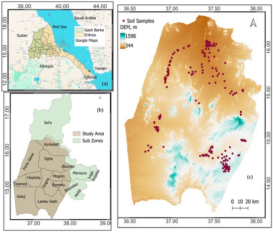
Figure 1.
Location map of Eritrea and Gash Barka administration zone (a), Gash Barka subzones and the study area (b), soil samples and digital elevation model (DEM) imposed on the study area (c), mean monthly temperature (d), annual rainfall (e), NDVI (f) of the study area.
The climate of the study area is predominantly arid [] with mean monthly temperatures ranging from 23.7 to 29.4 °C and annual rainfall varying between 184 and 680 mm []. Temperature increases from South to North, while rainfall exhibits the opposite trend, decreasing from South to North (Figure 1d,e). The topography predominantly consists of flat lowland plains with deep soils. Elevation generally decreases from South to North and from East to West (Figure 1c). The crop growing season is very short where most of the time rain starts late and ends early; the rainy season expands from early July to early September.
The study area predominantly practices extensive subsistence rainfed agriculture, characterized by mixed crop-livestock and agro-pastoral systems in most parts, with pastoralism prevailing primarily in the northern regions. Thirty years of data (1992–2021) from the Ministry of Agriculture (MoA) indicate that sorghum is the dominant crop, occupying 72.26% of the cultivated area, followed by pearl millet (12.52%), sesame (8.33%), and finger millet (1.68%), among others. Crop productivity remains low, with average yields (t ha−1) of rainfed sorghum at 0.52, pearl millet at 0.32, and sesame at 0.33. Livestock rearing is also widespread, with herds of camels, cattle, sheep, and goats commonly observed. These animals often overgraze the land, contributing to land degradation, as they freely move in search of pasture and water.
The construction of numerous micro- and macro-dams in the study area has promoted irrigated agriculture, enabling the cultivation of various vegetables, fruits, and crops such as banana, tomato, onion, hot pepper, cotton, teff, leafy vegetables, and others. Irrigation using groundwater along the banks of the Barka, Sawa, and Gash Rivers, as well as their tributaries, is also practiced. However, crop productivity remains low; for example, average yields for key irrigated crops—onion, banana, and tomato—are 20, 26, and 25 t ha−1, respectively (MoA records).
The area hosts a diverse range of plant and animal species [,]. However, biodiversity is progressively declining due to both anthropogenic and natural disturbances, with agricultural expansion being a primary driver []. Most of the study area is characterized by bare soils or scattered Acacia trees and shrubs, particularly in the western, central, and northern regions. The soils predominantly consist of Fluvisols, Leptosols, Lixisols, Vertisols, and Cambisols, which have been conventionally cultivated and grazed for centuries. Cultivation occurs during the rainy season, followed by heavy grazing after harvest, leaving the soils bare for the remainder of the year. Deforestation rates are high in the study area, with several studies reporting hotspots of declining annual and seasonal NDVI trends [], land productivity decline [], and serious desertification []. The NDVI map of the area (Figure 1f) indicates that vegetation cover is sparse across most of the study area. However, patches of Acacia trees and shrubs are commonly found in the southern regions, along with riverine forests lining the riverbanks.
2.2. Soil, Taxonomic, Geologic, and Land Use Data
In this study, we proposed a range of soil, land use, taxonomic, geological, topographic, climatic, Landsat 8 spectral bands, and spectral index variables as predictors of SOC in the study area, which are discussed below.
Three soil datasets were utilized in this study: (1) soil samples collected during the current study, (2) soil samples obtained from the Regulatory Service of the Ministry of Agriculture (MoA), and (3) legacy soil data from the soil laboratory of the National Agricultural Research Institute (NARI).
A total of 92 georeferenced composite surface soil samples (0–30 cm) were collected between September and November 2023 from various land uses and topographic settings using a 30 cm soil auger, following a stratified sampling technique [,]. Each composite sample was formed by collecting five subsamples within a 10 m radius, which were thoroughly mixed, packed, and labeled. The geographic coordinates (latitude and longitude) were recorded at the center of each sampling point.
The soil samples were air-dried, ground, and sieved according to standard procedures at the Soil Laboratory of Hamelmalo Agricultural College, Hamelmalo, Eritrea. They were analyzed for soil pH (using a pH meter) [], electrical conductivity (using an EC meter) [], and particle size distribution (via the hydrometer method) []. Soil organic carbon (SOC) was analyzed using the wet oxidation method [] as modified by [] at the Soil Laboratory of the National Agricultural Research Institute (NARI), Halhale, Eritrea. Additionally, key informant interviews were conducted during the soil sampling campaign to gain a deeper understanding of resource management practices, particularly those related to soils, within the study area.
Georeferenced surface soil samples (0–30 cm; n = 31) were also collected by the Regulatory Service of the Ministry of Agriculture (MoA) from small-scale farmers’ irrigated fields along the banks of the Sawa River. These samples were primarily intended to assess general soil conditions, with particular emphasis on salinity. Sampling, preparation, and laboratory analysis followed the same procedures described earlier. All laboratory analyses were conducted at the Soil Laboratory of the National Agricultural Research Institute (NARI), Halhale. During sampling, interviews were also conducted with farmers to gain insights into soil and water management practices.
In addition, legacy soil data were obtained from the NARI Soil Laboratory. These samples were collected mainly from government-managed large-scale irrigated farms, including Kerkebet, Afhimbol, Fanco, Adi Omer, and Gerset—as well as surrounding grazing lands and rainfed farming systems. From this dataset, only georeferenced surface samples (0–30 cm) with recorded SOC values were extracted, as the dataset also included subsurface samples and entries with missing SOC values or geographic coordinates.
The three datasets were compiled and subjected to Z-score analysis to identify and exclude outliers exceeding ±2 standard deviations. The final dataset consisted of 204 SOC data points, each with associated values for clay, silt, sand, soil texture, pH, electrical conductivity (EC), and geographic coordinates (latitude and longitude).
Parent material has great influence on soil formation and development, and thus, different studies employed soil taxonomy and geology in SOC studies [,]. Thereby, geology and soil taxonomy were included in the study. Soil taxonomy data were extracted from the Harmonized World Soil Database (HWSD) v2.0 []; Eritrea currently lacks a national soil map and an established soil classification system. In this study, five soil taxonomic units were identified—Cambisols, Lixisols, Leptosols, Fluvisols, and Vertisols—which were numerically coded as 1, 2, 3, 4, and 5, respectively, to convert the categorical data into a quantitative format suitable for modeling. Additionally, geological information was extracted from the national geological map of Eritrea developed by the Ministry of Energy and Mines (MoEM). The identified geological units included gneiss-based formations, alluvial deposits, intrusive rocks-based, meta-volcanic rocks-based, and late basin development-based sediments. These were also numerically coded as 1, 2, 3, 4, and 5, respectively.
Land use/land cover is an important factor that affects soil, and is commonly incorporated in SOC studies [,,,,]. Accordingly, land use and land use history data were recorded during soil sampling for most locations. For samples with missing land use information, land use types were identified based on prior knowledge of the study area and verified using Google Earth Pro. Four primary land use types were identified: communal grazing (CG), rainfed farming (RF), irrigated farming (IF), and natural forest (NF), and were numerically coded as 1, 2, 3, and 4, respectively.
In this context, communal grazing (CG) refers to areas used for year-round livestock grazing, excluding regions with significant natural forest cover. Natural forest includes areas with a well-developed forest canopy, even if they fall within communal grazing zones. Rainfed farming fields are also subject to communal grazing during the dry season. Figure 2 presents photographs of different land use types, taken during the soil sampling.
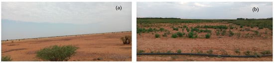
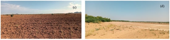
Figure 2.
Photos (November 2023) showing grazing land around Mogorayb (a), poorly managed drip-irrigated cotton crop at Kerkebet farm (b), rainfed field around Kerkebet farm (c), and River Barka and its riverine ecosystem around Afhimbol (d).
2.3. Topographic, and Climatic Data
Topography plays a critical role in soil formation and distribution; consequently, many studies have incorporated topographic variables into their SOC prediction models [,,,]. The dominant topography of the study area consists of flat lowland plains; therefore, topographic influence on soil properties is expected to be limited. Nonetheless, to assess the potential impact of topography on SOC variability, several topographic variables were included in the analysis. The elevation within the study area ranges from 1598 to 344 m above sea level and exhibits variation in slope, aspect, and other terrain characteristics. Topographic variables were derived from the ASTER Digital Elevation Model (DEM) of Eritrea and included: altitude, slope, aspect, topographic position index (TPI), LS factor (slope length and steepness), terrain roughness index (TRI), surface roughness, hill shade, sediment balance, upslope slope, negative openness, and positive openness.
Climate variables, particularly rainfall and temperature are among the most frequently used predictors in SOC studies, as these factors exert dominant influence on soil formation, organic matter decomposition, and carbon dynamics [,,,,,]. In this study, long-term historical rainfall and temperature data were extracted from the WorldClim 2.1 dataset (30 arc-seconds resolution), available at https://www.worldclim.org/data/worldclim21.html# (accessed on 3 September 2025) []. This approach was necessary due to the scarcity of long-term recorded climate data in Eritrea, and particularly within the study area.
2.4. Landsat 8 and Spectral Indices Data
We downloaded four L8 images with (path, row, dated) of (170, 049, 17 April 2024), (170, 050, 29 February 2024), (171, 049, 8 April 2024), and (171, 050, 8 April 2024) from the USGS archives https://earthexplorer.usgs.gov/ accessed on 24 May 2024. We chose images with <10% cloud cover in the dry months of February to April to avoid the interferences of clouds and seasonal vegetation. We computed different spectral indices using their respective formula (Table 2) using the raster calculator in QGIS 3.38. These spectral indices were normalized difference vegetation index (NDVI), infrared percentage vegetation index (IPVI), optimized soil adjusted vegetation index (OSAVI), modified SAVI2 (MSAVI2), normalized difference water index (NDWI), normalized difference soil index (NDSI), bare soil index (BSI), hyperspectral BSI (HBSI), soil organic carbon index (SOCI), normalized difference moisture index (NDMI), burn ration (BR), BR2, colouration index (CI), hue index (HI), and brightness index 2 (BI2). Different studies employed these spectral indices in different combinations [,,,,].
L8 bands B1, Blue, Green, Red, NIR, SWIR1, SWIR2, and B10 [,,] were also included with the dataset as potential SOC predictors.
The initial dataset consisted of 48 input variables. To eliminate both redundant and non-significant predictors, a preliminary Spearman correlation analysis was conducted, as it accounts for both linear and non-linear relationships. Variables that did not show a statistically significant correlation with SOC (p > 0.05) were excluded. Additionally, among pairs of variables that were perfectly correlated, one variable from each group was removed to avoid redundancy. As a result, the number of input variables was reduced to 36 (Table 1), which were retained as potential SOC predictor variables. Further refinement to address multicollinearity is described in Section 2.6.

Table 1.
Proposed potential SOC predictor variables after preliminary Spearman correlation analysis.
Table 1.
Proposed potential SOC predictor variables after preliminary Spearman correlation analysis.
| Variable Type | Variables, and Their Short Form, If Given | Resolution | Source |
|---|---|---|---|
| Soil properties | Clay, Silt, Sand, Texture, pH | 10 m | Lab measurement |
| Land use | Land Use (LU) | 10 m | LU history |
| Soil Taxonomy | Taxonomy (Taxom) | 1 km | HWSD v2.0 |
| Geology | Geology (Geogy) | 1 km | MoEM |
| Topography | Altitude (Alt), Slope, LS Factor (LSfctr), TRI, Roughness (Rough), Negative Openness (NvOp), Positive Openness (PvOp), Upslope Slope (UspSp), | 30 m | ASTER GDEM |
| Climate | Temperature (Temp), Rainfall (Rain) | 1 km | WorldClim 2.1 |
| L8 bands | B1, Blue, Green, Red, NIR, SWIR1, SWIR2 B10 | 30 m 100 m | L8—OLI sensor L8—TIRS sensor |
| Spectral Indices | NDVI, OSAVI, MSAVI2, NDWI, NDSI, HBSI, SOCI, NDMI, BR2, BI2 | 30 m | Computed |
Table 2.
Proposed potential SOC predictor spectral indices, and their formula.
Table 2.
Proposed potential SOC predictor spectral indices, and their formula.
| Spectral Index and Formula | Reference | Formula No. |
|---|---|---|
| NDVI = (NIR − Red)/(NIR + Red) | [] | (1) |
| OSAVI = (NIR − Red)/(NIR + Red + 0.16) | [] | (2) |
| MSAVI2 = 0.5 [2 × NIR + 1 − √ [(2 × NIR + 1)2 − 8(NIR − Red)]] | [] | (3) |
| NDWI = (Green − NIR)/(Green + NIR) | [] | (4) |
| NDSI = (SWIR1 − Green)/(SWIR1 + Green) | [] | (5) |
| HBSI = [(SWIR2 + Green) − (NIR + Blue)]/[(SWIR2 + Green) + (NIR + Blue)] | [] | (6) |
| SOCI = Blue/(Red × Green) | [] | (7) |
| NDMI = (NIR − SWIR1)/(NIR + SWIR1) | [] | (8) |
| BR2 = (SWIR1 − SWIR2)/(SWIR1 + SWIR2) | [] | (9) |
| BI2 = √ [(Red2 + Green2 + NIR2)/2] | [] | (10) |
2.5. Selection of Machine Learning Algorithms
Modelling the relationship between continuous independent variables and a continuous dependent variable typically involves regression fitting, which may take various functional forms such as linear, logarithmic, exponential, or power functions depending on the nature of the relationships. To accommodate these diverse relationships, we employed both linear regression-based and decision tree-based machine learning models. Specifically, we evaluated the performance of six algorithms: Multiple Linear Regression (MLR), Partial Least Squares (PLS), Cubist, Random Forest (RF), Gradient Boosting (GB), and Extreme Gradient Boosting (XGBoost). This approach enabled a comprehensive comparison of model performances and facilitated the identification of robust alternative models for SOC prediction.
MLR model is based on fitting many independent variables linearly to a dependent variable. The model has broad applicability in SOC prediction [,,,], though it is not robust with multicollinearity and outliers. PLS, a linear relationship-based model, focuses on maximizing covariance between predictors and responses, and seems robust with multicollinearity. This model is commonly used in SOC prediction modeling, and its performance is satisfactory [,,,].
Decision tree ensemble machine learning algorithms are generally more robust to multicollinearity and outliers compared to traditional regression methods. The Cubist model, a rule-based algorithm, combines decision trees with multiple linear regression models []. For each rule, a regression model is fitted based on the subset of data defined by that rule. These rules are hierarchically organized, where recursive partitioning of the response variable is performed to minimize the standard deviation across all potential splits []. The Cubist model is widely applied in SOC modeling and has consistently demonstrated strong predictive performance [,,,].
Random Forest (RF), introduced by [], constructs multiple decision trees by bootstrapping samples from the training dataset and subsequently aggregates their outputs to form a robust predictive model []. This ensemble approach reduces overfitting, improves model accuracy, and decreases computational time compared to individual trees. RF is widely applied across various data mining fields, including SOC modeling, due to its strong predictive performance and robustness [,,,,,,].
GB is a powerful ensemble learning model that builds models in a sequential manner where each new model corrects the errors made by the previous ones. It combines multiple weak learners to create a strong learner through boosting. It uses the concept of gradient descent to minimize the loss function. This model is also commonly used in SOC prediction studies [,,].
XGBoost is also a decision tree-based ensemble model [], advantaged by boosting algorithm. It tries to punish the weak learners and develop strong learners. Through parallel learning, computing speed is improved and over-fitting is prevented effectively. XGBoost model is gaining popularity in DSM [,,].
2.6. Selection of Input Variables
Utilizing a large number of input variables in predictive modeling may result in inaccurate conclusions due to multicollinearity among certain independent variables. Therefore, the selection of appropriate input variables is essential for developing robust predictive models [,]. This enhances model performance by mitigating multicollinearity and reducing model complexity, thereby facilitating faster model calibration []. In DSM, two approaches are commonly employed for covariate selection: (1) Selecting key covariates prior to modeling using correlation analysis or principal component analysis [,], which are based on linear relationships and may overlook covariates with nonlinear associations with the target variable [,]; (2) Feature importance ranking based on the model during calibration [,,], which is rooted in nonlinear relationships, but may introduce multicollinearity effects. While most studies have employed one of these approaches, few have compared their impacts on model performance, despite findings suggesting that both approaches are effective for variable selection [,].
In this study, we employed both approaches to compare their performance: (1) multicollinearity reduction using Spearman rank correlation, and (2) feature selection based on the Boruta algorithm. Multicollinearity between input variables was progressively reduced based on their correlations with each other and the target variable, as outlined below.
- In the first step, we executed the SOC modeling with all proposed input variables (36 variables) (Table 1).
- Based on Spearman correlation, we identified each set of variables that were very highly correlated (≥0.900 **) with each other, and we omitted the variable with weaker correlation with SOC by keeping the one with higher correlation with SOC []. For example, the correlation SWIR2 vs. SWIR1 = 0.975 ** (very high collinearity), and SWIR2 vs. SOC = −0.534 **, and SWIR1 vs. SOC = −0.505 **. Thus, SWIR2 is retained for the fact that it has higher correlation with SOC than SWIR1 (−0.534 ** vs. −0.505 **) but SWIR1 is removed.
- From each set of input variables that had high correlation (≥0.700 ** but <0.900 **) with each other, we omitted the variable with weaker correlation with SOC by keeping the one with the higher correlation with SOC.
- The Boruta feature selection wrapper algorithm was employed to select from the 36 proposed input variables. The algorithm is among the commonly used feature selection techniques in SOC prediction studies [,].
2.7. Calibration, Validation and Evaluation of Models
Figure 3 presents the conceptual flowchart of the methodologies employed. The models were trained, calibrated, and validated based on the extraction of independent SOC predictor variables to estimate target SOC values. The SOC modeling process was executed using Python 3.11.7 in the Jupyter Notebook environment. The dataset was randomly partitioned into training (80%) and testing (20%) subsets. We tested multiple algorithms, including MLR, PLS, Cubist, RF, GB, and XGBoost. Hyperparameter tuning and refinement were performed for each algorithm, with the exception of MLR, to optimize model performance, with particular emphasis on minimizing model discrepancies. Models were fitted, trained, calibrated, and validated, and their performance was assessed using commonly established metrics: RMSE, R2, RPD [,,,], and model discrepancy (MD), as defined by Equations (11), (12), (13), and (14), respectively.
where n = number of SOC observations, Oi = observed SOC values, Pi = predicted SOC values, Ô = mean of observed SOC values, T = RMSE of the training data, and t = RMSE of the testing data
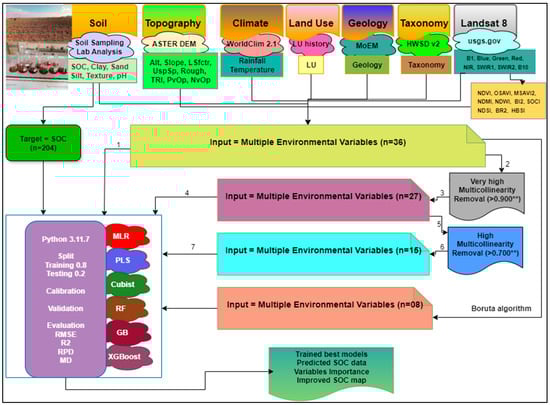
Figure 3.
Conceptual flowchart of the methodologies used; ** indicates significant at 0.01.
Furthermore, models are categorized as per their RPD values as; very poor (RPD < 1), poor (1–1.4), fair (1.4–1.8), good (1.8–2.0), very good (2.0–2.5), and excellent (>2.5) [].
3. Results and Discussions
3.1. Statistical Analysis of Observed Soil Properties
The studied soils exhibited moderate clay and silt content and high sand content, with average percentages of 26.28%, 27.89%, and 46.11%, respectively (Table 3), showing significant spatial variability (CV = 53.92%, 45.19%, and 41.08%, respectively). Soil texture ranged from sandy loam to clay, with sandy loams (32.8%) and loams (24.5%) being the most dominant. The dominant soil order was Fluvisols (46.6%), followed by Lixisols (20.6%) and Leptosols (16.2%). The study area is a lowland region that receives substantial runoff and soil sediments from the surrounding highlands, which may influence soil formation processes.
The soils were non-saline but moderately alkaline, with mean EC and pH values of 0.20 dS m−1 and 8.45, respectively. A small proportion of soils in areas such as Adi Hakin, Tekombia, Fanco, Mogolo, and Kerkebet exhibited stronger alkalinity. This alkalinity is likely attributed to the calcareous nature of soils in arid regions [], where calcium carbonate tests can provide valuable insights for informed management strategies. It is also important to note that alkaline soils may exhibit deficiencies in micronutrients such as manganese, copper, zinc, and boron [,].
The SOC content of the soils ranged from 0.02% to 1.01%, with a mean of 0.43%, standard deviation (SD) of 0.27%, and coefficient of variation (CV) of 61.65% (Table 3). SOC content decreased from south to north, following a similar pattern to rainfall distribution, but inversely correlated with temperature across the study area. The Laelay Gash subzone (in the south) recorded the highest mean SOC content, while the Kerkebet subzone (in the north) had the lowest mean SOC content.
According to [,,], the SOC content is considered poor. This finding is consistent with other studies conducted within the country. For instance, Ref. [] reported low SOC levels at Laelay Gash (part of the study area), and Refs. [,,] observed similar trends in other regions. Factors such as conventional tillage practices, continuous monocropping, excessive crop residue removal, minimal organic matter addition, overgrazing, and soil erosion, likely contributed to the low SOC content [,,,].
Table 3.
Statistical analysis of observed soil properties.
Table 3.
Statistical analysis of observed soil properties.
| Parameter | Minimum | Maximum | Mean | Status | SD | CV, % | Skewness | Kurtosis |
|---|---|---|---|---|---|---|---|---|
| Sand, % | 5.80 | 87.50 | 46.11 | High | 18.94 | 41.08 | 0.22 | −0.77 |
| Clay, % | 4.50 | 62.50 | 26.28 | Moderate | 14.17 | 53.92 | 0.46 | −1.11 |
| Silt, % | 2.50 | 58.00 | 27.89 | Moderate | 12.60 | 45.19 | 0.00 | −0.41 |
| EC, dS m−1 | 0.03 | 1.29 | 0.20 | Non-saline | 0.24 | 121.46 | 3.06 | 9.77 |
| pH | 7.18 | 9.72 | 8.45 | Moderately alkaline | 0.62 | 7.33 | −0.13 | −0.60 |
| SOC, % | 0.02 | 1.01 | 0.43 | Poor | 0.27 | 61.65 | 0.37 | −1.13 |
SD = standard deviation, CV = coefficient of variation, Status is given based on [,,].
SOC can be improved through effective agronomic practices such as crop rotation, legume–cereal intercropping, crop residue retention, cover cropping, technology-supported agroforestry practices, push-pull technology, farmyard manure application, integrated and diverse organic farming systems, no/minimal tillage, and the incorporation of biochar or other organic amendments.
In regions with limited natural vegetation, such as the study area, organic amendments play a critical role in enhancing soil fertility. Two abundant organic sources—Prosopis juliflora and organic municipal waste—are yet underutilized in the study area, and across the country. Integrating these resources into farming systems could yield multiple benefits, including improvements in food and nutrition security, as well as positive ecological, socio-economic, health, and environmental outcomes. Therefore, promoting composting and biochar technologies using these resources, alongside pilot research initiatives, is crucial.
Given that the study area is impacted by overgrazing, managing the appropriate stocking rate, implementing rotational grazing, allowing sufficient rest periods for pastures, establishing enclosures, promoting cut-and-carry methods, reseeding with legumes, and developing and utilizing grazing and SOC dynamics models [,] could significantly enhance soil health and fertility.
3.2. SOC Along Land Uses, Soil Taxonomic Units, and Irrigated Farms
The mean SOC values for the observed land use types were ranked as follows: natural forests (NF) > rainfed farming (RF) > irrigated farming (IF) > communal grazing (CG), with respective values of 0.66%, 0.48%, 0.42%, and 0.33% (Figure 4). The ANOVA test revealed that land use had a highly significant effect (p < 0.001) on SOC. However, the Tukey HSD post hoc test indicated no statistically significant difference in SOC between IF and RF, as well as between IF and CG land uses. These results suggest that NF has the potential for soil carbon (C) sequestration, whereas the other land uses are more likely to contribute to soil C release. Ref. [] also emphasized the importance of conserving and enhancing natural forests for C sequestration, while highlighting the risks associated with RF and CG land uses, which may contribute to C release into the atmosphere.
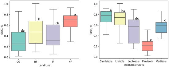
Figure 4.
Effect of land use (left), and soil taxonomic units (right) on SOC; lowercase letters indicate which specific group means are different after conducting ANOVA test.
Our results contradict with the findings that reported significantly higher SOC contents in irrigated farming (IF) compared to rainfed farming (RF) and communal grazing (CG) land use types [,]. Ref. [] emphasized the importance of IF for carbon storage in Keren, Eritrea. In general, numerous studies have highlighted the significant effect of land use on SOC levels [,,,,].
Based on the interviews with farmers and key informants, along with general observations during soil sampling, it is evident that agronomic and soil management practices in the study area are suboptimal. Soil nutrient depletion is pronounced due to extensive grain and biomass harvesting, coupled with overgrazing and minimal organic matter inputs. Furthermore, irrigated soils are cultivated 2–3 times per year with little to no nutrient replenishment, exacerbating nutrient depletion. Crop biomass is primarily harvested and either fed to livestock or sold for cash. In this arid environment, vegetation is scarce, rangelands and crop fields are overgrazed shortly after the autumn harvest, and the harvested crop biomass constitutes the primary feed for livestock during the winter and spring seasons across much of the study area.
The mean SOC values for the soil taxonomic units were ranked as follows: Cambisols > Lixisols > Vertisols > Leptosols > Fluvisols, with respective values of 0.75%, 0.72%, 0.56%, 0.50%, and 0.22% (Figure 4). The ANOVA test revealed that soil taxonomy had a highly significant effect (p < 0.001) on SOC. However, the Tukey HSD post hoc test indicated no significant difference in SOC between Cambisols and Lixisols, nor between Vertisols and Leptosols. Fluvisols exhibited the lowest mean SOC, with most of the sampled Fluvisols located along the banks of the Barka and Sawa Rivers in the northern part of the study area. The low SOC in Fluvisols may be more attributable to the regional climate rather than the inherent properties of the soils, a conclusion that aligns with the findings presented in Section 3.5 on the importance of variables.
Table 4 presents the descriptive statistics of SOC in the irrigated farms. All the irrigated farms, whether government or privately operated, exhibited low SOC content, primarily due to inadequate agronomic and soil fertility management practices. Common issues include mono-cropping, nutrient depletion through frequent grain and crop residue harvesting (2–3 times per year) with minimal nutrient replenishment. Additionally, deep nutrient and water percolation may significantly impact SOC levels, as most farms rely on furrow irrigation systems, despite the soils being sandy and permeable. Furthermore, the practice of deep ploughing with heavy tractors and discs exacerbates nutrient losses. To address these challenges, awareness campaigns and training programs on proper tillage practices, soil nutrient and irrigation water management, crop rotation, legume–cereal intercropping, agroforestry practices, cover cropping, green manuring, composting, and the application of bio-fertilizers and biochar technologies are essential for farmers and land managers in the study area.
Table 4.
Descriptive statistics of SOC in irrigated farms.
Farms in the northern part of the study area (Kerkebet, Afhimbol, and Forto Sawa) exhibited relatively lower mean SOC contents compared to farms in other regions. The highest and lowest mean SOC values were recorded at Shambko farms (in the southeast) and Afhimbol farm (in the north), with values of 0.73% and 0.14%, respectively. These differences are likely attributed to climatic variations rather than differences in farm management practices.
3.3. Correlation Analysis, and Multicollinearity Reduction
Spearman correlation analysis revealed that most of the input variables showed strong correlations with SOC (Figure 5). Rainfall (0.746 **) exhibited the highest correlation with SOC, followed by temperature (−0.732 **), altitude (0.729 **), NIR (−0.640 **), Green (−0.632 **), SOCI (0.612 **), BI2 (−0.609 **), Red (−0.591 **), Blue (−0.589 **), and Sand (−0.573), among others. These results suggest that climate factors, specifically rainfall and temperature, may have the greatest impact on SOC and may offer strong predictive capacity for SOC in the study area. Altitude also serves as a surrogate for climate, as higher altitudes generally correspond to cooler temperatures and vice versa.
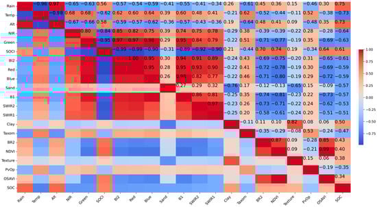
Figure 5.
Correlation heatmap: only 20 input variables are displayed (due to limited display space), arranged in decreasing magnitude of their correlations with SOC.
Following the climate variables, L8 bands and bare soil indices demonstrated strong potential for SOC prediction. Soil attributes like sand and clay content, as well as soil taxonomy, also exhibited good correlations with SOC and may contribute significantly to SOC prediction. However, land use, geology, and topographic variables showed relatively lower correlations with SOC and likely exert less influence on it.
Many of the input variables exhibited very high correlations (≥0.900 **) with each other, necessitating multicollinearity reduction. For example, rainfall, temperature, and altitude were highly correlated, and only rainfall was retained due to its stronger correlation with SOC compared to the other two. Similarly, very high correlations were observed among Green, B1, Blue, Red, BI2, and SOCI, and only the Green band was retained. As a result, nine variables—temperature, altitude, B1, Blue, Red, SWIR1, BI2, SOCI, and OSAVI—were removed due to high multicollinearity with other input variables. Consequently, the number of input variables was reduced from 36 to 27.
High correlations (≥0.700 **) were also observed between different groups of the independent variables. Accordingly, 12 variables were omitted at this step; Green, SWIR2, clay, NDVI, MSAVI2, HBSI, NDWI, NDSI, slope, LS factor, TRI, and roughness, and the input variables were reduced to 15.
According to the Boruta feature selection algorithm, eight variables were selected from the 36 proposed input variables: rainfall, sand, taxonomy, clay, SWIR2, SOCI, Green, and temperature. SOC modeling was then conducted using four categories of input variables: 36, 27, 15, and 8. Based on the Boruta algorithm, the importance score for rainfall was dominant (>0.6), while none of the other variables had an importance score greater than 0.1 (Figure 6), highlighting the significant influence of rainfall on SOC in the study area.
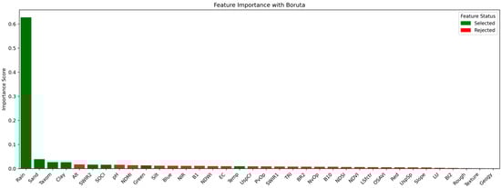
Figure 6.
Feature importance score and selection using the Boruta algorithm: selected (green), rejected (red).
3.4. Performance of Models
The observed SOC ranged, in %, 0.02–1.01 with a mean = 0.43, SD = 0.27, and CV = 61.65%, and that of the training and testing SOC varied 0.02–1.01, and 0.04–0.85, with means of 0.44, and 0.39, respectively (Table 5). Generally, the soils had low SOC, and showed high spatial variation (CV > 60%), which high spatial variation may challenge SOC modeling.
Table 5.
Statistics of total (observed), training and testing SOC (%).
The performance of the examined models with different input variables to the training and testing data is shown in Table 6. All models fit well to both data types in all the varied number of input variables. For the training data, the highest performance was achieved by the MLR_36 model (MLR model with 36 input variables) with an RMSE of 0.114, R2 of 0.824, and RPD of 2.342. However, its model discrepancy (MD) was 21.71%, which is high enough to logically question this model. Thus, the highest credit was taken by the XGB_36 model (XGBoost model with 36 input variables) with RMSE = 0.115, R2 = 0.818, RPD = 2.308, and MD = 3.99%. The lowest model performance was recorded by the PLS_08 model with RMSE = 0.135, R2 = 0.731, RPD = 1.964, and MD = 3.43% (Table 6, Figure 7a,c). Figure 7 displays the RMSE, RMSE change, and MD of the models with different input variables.
Table 6.
Performance of models for the training and testing data with different number of input variables.
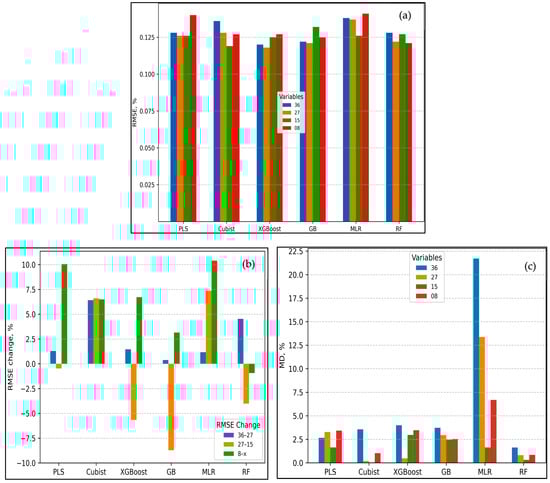
Figure 7.
RMSE (a), RMSE change (b) and MD (c) with different input variables: RMSE Change (x stands for the lowest RMSE in each model; positive and negative changes indicate model enhancement and model deterioration, respectively).
For the validation data, the highest model accuracy was recorded by the XGB_27 model with an RMSE of 0.118, R2 of 0.758, RPD of 2.252, and MD of 0.48%, and on the contrary, the lowest was observed in the MLR_08 model with RMSE = 0.141, R2 = 0.742, RPD = 1.883, and MD = 6.68 (Table 6, Figure 7a,c). The XGBoost model is a powerful and efficient gradient boosting algorithm that is gaining popularity in many fields including SOC prediction. Different authors also confirmed that the XGBoost model performed the best in their SOC prediction studies [,,]. Generally, the accuracies obtained are on the average of most of DSM and SOC prediction modeling reports [,,,,].
The highest model discrepancy (MD), 21.71%, was observed in the MLR_36 model, followed by the MLR_27 model (13.38%). This can likely be attributed to the multicollinearity effect, as the MLR model does not address multicollinearity. The lowest MD, 0.02%, was observed in the Cubist_08 model. Overall, the Random Forest (RF) model exhibited the lowest MD, followed by the Cubist model. All models, except the MLR model, maintained an MD of less than 5% across all stages with different input variables (Figure 7c). MD is the difference in performance of a machine learning model when applied to training versus testing data, which is crucial for assessing how well a model generalizes to unseen data. The acceptable level of MD tolerance depends on the accuracy requirements of the target application.
According to their RPD values, most of the models were categorized as ‘very good’ for both datasets across all different input variable sets. The PLS and MLR models with 8 input variables showed relatively weaker performance but still fell within the ‘good’ model category, with an RPD > 1.80. RPD represents the factor by which prediction accuracy increases compared to using the mean of the original data. This indicates that all trained, calibrated, and validated models—except for the MLR_36 and MLR_27 models due to their high MD—demonstrated good SOC predictive accuracy. These models can be used for planning and monitoring soil fertility improvements, food production, carbon sequestration, and climate change mitigation.
All models showed improvements when the number of input variables was reduced from 36 to 27 (following the removal of very high multicollinearity), with the greatest improvement recorded by the Cubist model (6.42%), followed by the RF model (4.53%) (Figure 7b). This may indicate that removal of very high multicollinearity (≥0.900 **) is important for better model performance. However, when the number of input variables was reduced from 27 to 15 (after high multicollinearity removal), performance of most of the models deteriorated (GB, XGBoost, RF, and PLS), and only the MLR and Cubist models continued improving (Figure 7b). This may imply that high multicollinearity (≥0.700 ** but <0.900 **) removal may not be necessary especially for the models that deal well with multicollinearity.
In comparison to the Boruta algorithm-based selection of variables (08 input variables), all the models, except the RF model, benefited from the multicollinearity reductions. The highest model performance improvement was obtained by the MLR (10.41%) model followed by the PLS (10.06%), and the XGBoost (6.72%), respectively, and the lowest improvement was in the GB model (3.15%) (Figure 7b). This indicates the potential of Spearman rank correlation-based multicollinearity reduction to enhance performance of models.
During the calibration, and validation of models, the following hyperparameters settings were used: Cubist (n_committees = 100, n_rules = 2), RF (max_depth = 3, min_samples_split = 2, min_samples_leaf = 2), GB (learning_rate = 0.07, max_depth = 1, min_samples_split = 7), XGBoost (colsample_bytree = 0.9, max_depth = 1, learning_rate = 0.07, subsample = 0.7), PLS (n_components = 26, 16, 15, 5, respectively), and no hyperparameter was used with the MLR model.
3.5. Importance of Variables
Variable importance rankings from the XGBoost, Random Forest (RF), and Gradient Boosting (GB) models revealed that, across all categories of input variables, rainfall was the most important variable for SOC prediction in the study area. In some cases, rainfall alone explained more than 60% of the SOC variance, particularly with the GB model.
According to the XGBoost_36 model, the top five most important variables for SOC prediction were rainfall, temperature, taxonomy, altitude, and SWIR2, which together accounted for 73.61% of the SOC spatial variation in the study area. Notably, rainfall alone explained 32.62% of the SOC variance (Figure 8a). Similarly, the RF_36 model identified rainfall, temperature, altitude, taxonomy, and NIR as the top five variables, accounting for 66.32% of SOC variability, with rainfall explaining 20.48% of the variance (Figure 8b). In the GB_36 model, the top five variables were rainfall, altitude, sand, SWIR2, and taxonomy, collectively explaining 92.17% of the variance in SOC, with rainfall contributing the largest share, 58.28% (Figure 8c).
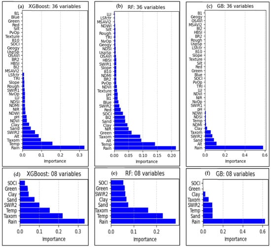
Figure 8.
Variables importance for SOC prediction: XGBoost, RF, and GB models with 36 and 08 variables.
Climate through rainfall (mainly), temperature, and altitude was identified as the first to have the highest impact on SOC in the study area. Altitude is a surrogate variable for climate. From the Spearman correlation analysis, we also realized that SOC had the highest correlation with rainfall followed by temperature and altitude. Moreover, these three variables had very high correlation (>0.900 **) with each other, which shows that they can substitute each other. Different studies in different regions also reported that climate had the highest influence on SOC [,,,,,].
Similar trends were observed with the 27, 15 and 08 input variables that rainfall occupied the first place in all with the XGBoost, RF, and GB models. Moreover, the importance of rainfall increased as the number of input variables decreased. For instance, rainfall addressed 33.41, 28.51, and 62.50% of the SOC variation according to the XGBoost, RF, and GB models with 08 input variables, respectively (Figure 8d–f). Thus, rainfall has the greatest SOC predictive capacity in the study area.
Figure 9 summarizes the average variables importance for the XGBoost, RF and GB models with 36 variables. It also distinguishes different variable types through different colours. The first most important variable was rainfall and addressed 37.13% of the SOC variance. The second most important SOC predictor variable was altitude (12.00%) followed by temperature (11.36%), taxonomy (7.96%), SWIR2 (5.73%), sand (5.65%), clay (2.87%), NIR (2.09%), pH (1.25%), and NDVI (1.09%), respectively, among others.
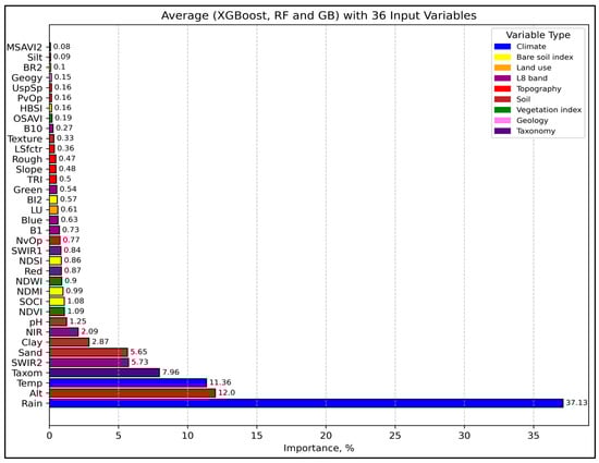
Figure 9.
Average variables importance for SOC prediction of the XGBoost, RF, and GB models with 36 variables.
Climate, mainly through rainfall, and secondly through temperature, and altitude, holds the highest influence (60.48%) on SOC in the study area. This finding agrees with the findings of [,] who reported that rainfall dictates the vegetation dynamics in the country, and [] also stated that rainfall is crucial variable for deforestation and desertification studies in the country. Since the 1960s, in the country, the frequency of moderate and extreme droughts has increased [] and temperature has risen in the past 6 decades by about 1.7 °C, which has led to climate change with great loss impacts on agricultural production, biodiversity and overall ecosystem resilience []. A comprehensive analysis on East African agriculture and climate change by [] also presented decreasing rainfed sorghum yield due to climate change in the study area. Thus, adoption of climate-smart agriculture that enhances soil moisture and minimizes water loss could be effective in the study area. In this essence, the country’s widespread campaigns on soil and water conservation are encouraged. However, monitoring and evaluation is needed for more effective and efficient actions.
Soil nature (taxonomy, sand, and clay) and L8 spectral bands (SWIR2, NIR) had also good capacity of SOC prediction in the study area. Sand is mostly correlated to SOC negatively as coarse texture is the sign of removal of fine particles by soil deflation, and clay holds the opposite. Thus, these two particles are important indicators of SOC status. Moreover, SWIR2 and NIR are sensitive to soil moisture and soil organic matter [] and are important SOC predictors. Land use, geology, vegetation indices, bare soil indices, and topographic variables showed weak SOC predictive capacity.
3.6. SOC Mapping
Here, we selected the best one from each model and presented their predicted SOC (Table 7). In all models the SD, CV and skewness of the predicted SOC were reduced as compared to the observed SOC. The lowest CV (50.00%) was recorded by the RF_08 model and the highest CV (56.39%) by the PLS_27 as opposed to 61.65% for the observed SOC. The XGBoost, GB, and RF models gave relatively lower ranges between the minimum and maximum SOC values as compared to the MLR, PLS and Cubist models. Almost all the models fell short of predicting the minimum and maximum values, and the predicted SOC values were shrunk towards the mean. However, the PLS_27 model recorded a minimum SOC value of −0.02%, as opposed to 0.02% for the observed SOC.
Table 7.
Descriptive statistics of observed and predicted SOC.
Rainfall was found to be the main SOC deriver in the study area. Thus, we plotted scatter diagrams of rainfall versus predicted SOC and executed equations and R2 for each model (Figure 10). The R2 was the highest in polynomial relations in each model, and degree 2 quadratic equations were developed for each model. Predicted SOC in all models showed high correlation with rainfall; the highest R2 be 0.8485 for the MLR_15 and the lowest, 0.8172, for the PLS_27. These high correlations indicate the high possibility of calculating and mapping SOC as a function of rainfall using the equations developed in each model for the study area. Figure 10 displays scatter plots of rainfall versus predicted SOC from the selected models and their respective R2 and quadratic equations.
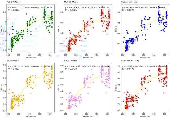
Figure 10.
Predicted SOC versus rainfall scatter plots, R2 and quadratic equations for the different models.
We generated continuous SOC maps using the equations we developed from the rainfall versus predicted SOC scatter plots of each model. These were done using the raster calculator in QGIS 3.38 having raster rainfall map of the study area and executing the equations. All the models showed similar pattern that predicted SOC increased from the North to the South in the study area (Figure 11) in the same pattern as the rainfall and altitude do, and vice versa as the temperature does. The MLR_15 and PLS_27 models showed relatively denser SOC values for the high SOC areas (southern part), and relatively lower SOC values for the low SOC areas (northern part) as compared to the other models. Generally, all the models revealed that the southern and southeastern parts had the highest and northern and northwestern parts had the lowest predicted SOC.
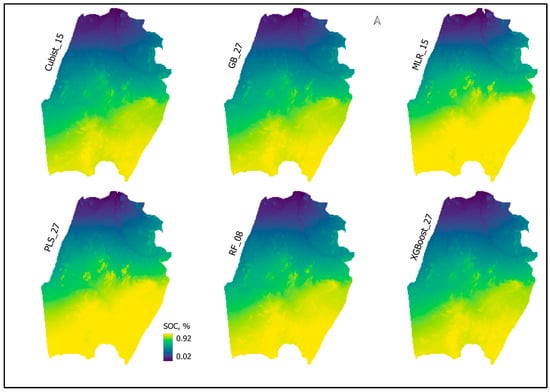
Figure 11.
SOC maps developed using the equations from the rainfall versus predicted SOC scatter plots in each model.
3.7. Comparison with the SoilGrids250m Product
Eritrea doesn’t have its own soil database, and it adopts the SoilGrids250m [] product [,], which is used for different purposes; for instance, national Land Degradation Neutrality (LDN) assessments and reports [,]. Global digital soil maps (DSM) such as the SoilGrids250m are useful assets. However, these may underestimate or overestimate targeted soil properties in regions where there were no/limited soil data for training such as most of the African countries including Eritrea. Thus, we compared our model (Predicted_RF), and SoilGrids250m SOC against the observed SOC. The mean SOC of the observed, predicted (RF model), and SoilGrids250m were 0.43, 0.44, and 0.99%, respectively (Figure 12). The mean observed and predicted SOC were statistically equal. However, the SoilGrids250m highly significantly overestimated the mean SOC. Moreover, the range between the minimum (0.00%) and maximum (2.06%) SOC for the SoilGrids250m was large. Similar studies also reported that SoilGrids250m product overestimated SOC [,,,]. Thus, we have developed workable local SOC predictor models for the Western Lowlands of Eritrea, and the necessity for modeling SOC in other parts of the country seems urgent.
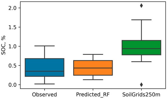
Figure 12.
Mean SOC according to Observed, Predicted_RF and SoilGrids250m models; extreme out layers (black diamond shapes) are shown within the SoilGrids250m indicating its high uncertainty for the study area.
3.8. Limitations of the Study
The study focused solely on the spatial distribution of SOC in surface soils (0–30 cm) using only one-time Landsat 8 images, along with other environmental covariates. This limited the analysis of subsurface soil layers and temporal dynamics of SOC. Additionally, the developed models may exhibit deficiencies due to the small amount of training data, variations in timing, and uneven soil sampling frames. Thus, to enhance the models further, it is essential to incorporate spatio-temporal dynamics of both surface and subsurface soils, utilizing multispectral and hyperspectral satellite images, along with other environmental covariates. This should include studies of climate scenarios with a larger and more evenly distributed set of soil samples in the study area, particularly in the context of a changing climate.
4. Conclusions
The soils of the Western Lowlands of Eritrea were non-saline with moderately alkaline pH, characterized by high sand content, moderate silt and clay, and low SOC (0.43%) content with high spatial variability. The low SOC levels require urgent attention due to their critical role in soil fertility, food production, ecosystem restoration, and climate change mitigation. Furthermore, SOC levels in grazing, rainfed, and irrigated farming land uses were poor and statistically similar, primarily due to suboptimal management practices that deplete soil nutrients. In contrast, natural forestlands exhibited significantly higher SOC, highlighting their potential for soil carbon sequestration. To address these challenges, it is essential to implement awareness-raising campaigns and training programs for farmers and land managers in the study area, focusing on soil nutrient and irrigation water management, crop rotation, legume–cereal intercropping, agroforestry practices, cover cropping, green manuring, composting, and the application of bio-fertilizers and biochar technologies.
The spatial distribution of SOC in the study area was modeled with high accuracy using MLR, PLS, Cubist, RF, GB, and XGBoost models. The XGBoost model with 27 input variables achieved the highest SOC prediction accuracy, with RMSE = 0.118%, R2 = 0.758, RPD = 2.252, and MD = 0.48%. In contrast, the MLR model with 8 input variables showed the lowest accuracy, with RMSE = 0.141, R2 = 0.742, RPD = 1.883, and MD = 6.68%. Rainfall emerged as the most significant predictor of SOC, explaining over 60% of the variance, while other important predictors included temperature, soil taxonomy, SWIR2, NIR, sand, and clay.
Reducing very high multicollinearity (>0.900**) proved beneficial for all models. However, a reduction in high multicollinearity (>0.700**) did not lead to improvements for the PLS, RF, GB, and XGBoost models. When compared to the Boruta algorithm-based variable selection, the multicollinearity reduction strategy resulted in notable model improvements for the MLR, PLS, XGBoost, Cubist, and GB models, with performance gains of 10.41%, 10.06%, 6.72%, 6.50%, and 3.15%, respectively.
We conclude that all the developed models, except for MLR_36 and MLR_27, demonstrated good accuracy and can be effectively utilized for the planning and monitoring of soil fertility and productivity improvements, ecosystem restoration, and climate change mitigation efforts. For more robust results, we recommend conducting additional SOC modeling studies with larger soil sample sizes from multiple areas and comparing a wider range of models, both in the study area and in other regions of the country.
Author Contributions
Conceptualization, T.T., E.S.M. and W.O.; methodology, T.T.; software, T.T.; validation, I.Y.S., T.T., E.S.M., D.E.K., N.Y.R. and W.O.; formal analysis, T.T.; investigation, T.T.; data curation, T.T.; writing—original draft preparation, T.T.; writing—review and editing, I.Y.S., E.S.M., D.E.K., N.Y.R. and W.O.; visualization, T.T.; supervision, E.S.M.; project administration, E.S.M., D.E.K. and N.Y.R. All authors have read and agreed to the published version of the manuscript.
Funding
This publication has been supported by the RUDN University Scientific Projects Grant System, project no. 202786-2-000.
Institutional Review Board Statement
Ethical review and approval were waived for this study by the Ministry of Health. Ethical clearance is only required for studies involving sensitive demographic, socio-economic, health, or cultural data, which was not applicable to this research. The study involved key informant interviews limited to general agricultural practices and natural resource management.
Informed Consent Statement
Informed consent was obtained from all subjects involved in the study.
Data Availability Statement
Data is available from the corresponding author upon formal and reasonable request.
Acknowledgments
The authors deeply acknowledge RUDN University; Ministry of Agriculture (MoA), Eritrea; National Agricultural Research Institute (NARI); Hamelmalo Agricultural College (HAC); and Eritrean Crops and Livestock Corporation (ECLC). Our great acknowledgements also go to the anonymous peer and editorial reviewers for their constructive comments.
Conflicts of Interest
The authors declare no conflicts of interest.
References
- FAO. Soil Organic Carbon: The Hidden Potential; Food and Agriculture Organization of the United Nations: Rome, Italy, 2017. Available online: https://openknowledge.fao.org/server/api/core/bitstreams/b382a255-5bd5-4656-a8cd-e30fff1a8bfe/content (accessed on 3 September 2025).
- Page, K.L.; Dang, Y.P.; Dalal, R.C. The ability of conservation agriculture to conserve soil organic carbon and the subsequent impact on soil physical, chemical, and biological properties and yield. Front. Sustain. Food Syst. 2020, 4, 31. [Google Scholar] [CrossRef]
- Kherif, O.; Keskes, M.I.; Pansu, M.; Ouaret, W.; Rebouh, Y.N.; Dokukin, P.; Kucher, D.; Latati, M. Agroecological modelling of nitrogen and carbon transfers between decomposer micro-organisms, plant symbionts, soil and atmosphere in an intercropping system. Ecol. Model. 2021, 440, 109390. [Google Scholar] [CrossRef]
- Tan, Z.X.; Lal, R.; Smeck, N.E.; Calhoun, F.G. Relationships between soil organic carbon pool and site variables in Ohio. Geoderma 2004, 121, 187–195. [Google Scholar] [CrossRef]
- Pringle, M.J.; Allen, D.E.; Phelps, D.G.; Bray, S.G.; Orton, T.G.; Dalal, R.C. The effect of pasture utilization rate on stocks of soil organic carbon and total nitrogen in a semi-arid tropical grassland. Agric. Ecosyst. Environ. 2014, 195, 83–90. [Google Scholar] [CrossRef]
- Schulz, K.; Voigt, K.; Beusch, C.; Almeida-Cortez, J.S.; Kowarik, I.; Walz, A.; Cierjacks, A. Grazing deteriorates the soil carbon stocks of Caatinga forest ecosystems in Brazil. For. Ecol. Manag. 2016, 367, 62–70. [Google Scholar] [CrossRef]
- Tolimir, M.; Kresović, B.; Životić, L.; Dragović, S.; Dragović, R.; Sredojević, Z.; Gajić, B. The conversion of forestland into agricultural land without appropriate measures to conserve SOM leads to the degradation of physical and rheological soil properties. Sci. Rep. 2020, 10, 13668. [Google Scholar] [CrossRef]
- Don, A.; Schumacher, J.; Freibauer, A. Impact of tropical land-use change on soil organic carbon stocks–a meta-analysis. Glob. Change Biol. 2011, 17, 1658–1670. [Google Scholar] [CrossRef]
- Sanderman, J.; Hengl, T.; Fiske, G.J. Soil carbon debt of 12000 years of human land use. Proc. Natl. Acad. Sci. USA 2017, 114, 9575–9580. [Google Scholar] [CrossRef]
- Berhe, S.M. Final Country Report of the Land Degradation Neutrality Target Setting Programme in Eritrea. In The State of Eritrea; UNCCD National Focal Point: Bonn, Germany; LDN National Working Group, Ministry of Agriculture: Asmara, Eritrea, 2018. Available online: https://www.unccd.int/sites/default/files/ldn_targets/Eritrea%20LDN%20TSP%20Country%20Report.pdf (accessed on 3 September 2025).
- MoA. National Land Degradation Neutrality Targets; Ministry of Agriculture: Asmara, Eritrea, 2018. Available online: https://www.unccd.int/sites/default/files/ldn_targets/Eritrea%20LDN%20Country%20Commitments.pdf (accessed on 26 October 2022).
- Ghebrezgabher, M.G.; Taibao, Y.; Xuemei, Y.; Congqiang, W. Assessment of desertification in Eritrea: Degradation based on Landsat images. J. Arid. Land 2019, 11, 319–331. [Google Scholar] [CrossRef]
- Nuguse, M.T.; Singh, B.; Ogbazghi, W. Studies on soil organic carbon and some physico-chemical properties as affected by different land uses in Eritrea. J. Soil Water Cons. 2019, 18, 213–222. [Google Scholar] [CrossRef]
- Tesfay, T.; Ogbazghi, W.; Singh, B. Effects of soil and water conservation interventions on some physico-chemical properties of soil in Hamelmalo and Serejeka Sub-zones of Eritrea. J. Soil Water Cons. 2020, 19, 229–234. [Google Scholar] [CrossRef]
- Tesfay, T.; Mohamed, E.S.; Ghebretnsae, T.W.; Ghebremariam, S.B.; Mehrteab, M. Soil organic carbon stock assessment for soil fertility improvement, ecosystem restoration and climate-change mitigation. In Proceedings of the RIEEM 2024, E3S Web of Conferences, Moscow, Russia, 26–28 April 2024; Volume 555. [Google Scholar] [CrossRef]
- Tesfay, T.; Mohamed, E.S.; Medhanie, M.; Ghebretnsae, T.W.; Sereke, T.E. Soil organic carbon losses following conversion of natural forests into agriculture. Dokuchaev Soil Bull. 2025, 123, 100–115. [Google Scholar] [CrossRef]
- Tesfay, T.; Ogbazghi, W.; Singh, B.; Tsegai, T. Factors Influencing Soil and Water Conservation Adoption in Basheri, Gheshnashm and Shmangus Laelai, Eritrea. IRA Int. J. Appl. Sci. 2018, 12, 7–14. [Google Scholar] [CrossRef]
- Ghebrezgabher, M.G.; Yang, X. Spatio-temporal assessment of climate change in Eritrea based on precipitation and temperature variables. World Wide J. Multidiscip. Res. Dev. 2018, 4, 1–10. [Google Scholar]
- Ghebrezgabher, M.G.; Yang, T.; Yang, X.; Wang, X. Extracting and analyzing forest and woodland cover change in Eritrea based on Landsat data using supervised classification. Egypt J. Remote Sens. Space Sci. 2016, 19, 37–47. [Google Scholar] [CrossRef]
- Measho, S.; Chen, B.; Trisurat, Y.; Pellikka, P.; Guo, L. Spatio-Temporal Analysis of Vegetation Dynamics as a Response to Climate Variability and Drought Patterns in the Semiarid Region, Eritrea. Remote Sens. 2019, 11, 724. [Google Scholar] [CrossRef]
- Adhikari, K.; Hartemink, A.E.; Minasny, B.; Kheir, R.B.; Greve, M.B.; Greve, M.H. Digital mapping of soil organic carbon contents and stocks in Denmark. PLoS ONE 2014, 9, e105519. [Google Scholar] [CrossRef]
- Mohamed, E.S.; Saleh, A.M.; Belal, A.B.; Gad, A.A. Application of near infrared reflectance for quantitative assessment of soil properties. Egypt. J. Remote Sens. Space Sci. 2018, 21, 1–14. [Google Scholar] [CrossRef]
- Gouda, M.; Abu-hashim, M.; Nassrallah, A.; Khalil, M.N.; Hendawy, E.; Benhasher, F.F.; Shokr, M.S.; Elshewy, M.A.; Mohamed, E.S. Integration of remote sensing and artificial neural networks for prediction of soil organic carbon in arid zones. Front. Environ. Sci 2024, 12, 1448601. [Google Scholar] [CrossRef]
- Chen, Q.; Wang, Y.; Zhu, X. Soil organic carbon estimation using remote sensing data-driven machine learning. PeerJ 2024, 12, e17836. [Google Scholar] [CrossRef]
- Nguyen, T.T.; Pham, T.D.; Nguyen, C.T.; Delfos, J.; Archibald, R.; Dang, K.B.; Hoang, N.B.; Guo, W.; Ngo, H.H. A novel intelligence approach based active and ensemble learning for agricultural soil organic carbon prediction using multispectral and SAR data fusion. Sci. Total Environ. 2022, 804, 150187. [Google Scholar] [CrossRef] [PubMed]
- Meliho, M.; Boulmane, M.; Khattabi, A.; Dansou, C.E.; Orlando, C.A.; Mhammdi, N.; Noumonvi, K.D. Spatial prediction of soil organic carbon stock in the Moroccan high atlas using machine learning. Remote Sens. 2023, 15, 2494. [Google Scholar] [CrossRef]
- Suleymanov, A.; Tuktarova, I.; Belan, L.; Suleymanov, R.; Gabbasova, I.; Araslanova, L. Spatial prediction of soil properties using random forest, k-nearest neighbors and cubist approaches in the foothills of the Ural Mountains, Russia. Model. Earth Syst. Environ. 2023, 9, 3461–3471. [Google Scholar] [CrossRef]
- Devine, S.; O’Geen, A.; Liu, H.; Jin, Y.; Dahlke, H.; Larsen, R.; Dahlgren, R. Terrain attributes and forage productivity predict catchment-scale soil organic carbon stocks. Geoderma 2020, 368, 114286. [Google Scholar] [CrossRef]
- Zhou, T.; Geng, Y.; Chen, J.; Pan, J.; Haase, D.; Lausch, A. High-resolution digital mapping of soil organic carbon and soil total nitrogen using DEM derivatives, Sentinel-1 and Sentinel-2 data based on machine learning algorithms. Sci. Total Environ. 2020, 729, 138244. [Google Scholar] [CrossRef]
- Zhao, F.; Wu, Y.; Hui, J.; Sivakumar, B.; Meng, X.; Liu, S. Projected soil organic carbon loss in response to climate warming and soil water content in a loess watershed. Carbon Balance Manag. 2021, 16, 24. [Google Scholar] [CrossRef]
- Shen, C.; Xiao, W.; Chen, J.; Hua, L.; Huang, Z. Climate-Sensitive Spatial Variability of Soil Organic Carbon in Multiple Forests, Central China. Glob. Eco. Cons 2023, 46, e02555. [Google Scholar] [CrossRef]
- Zhou, Y.; Chartin, C.; Van Oost, K.; van Wesemael, B. High-resolution soil organic carbon mapping at the field scale in Southern Belgium (Wallonia). Geoderma 2022, 422, 115929. [Google Scholar] [CrossRef]
- Galluzzi, G.; Plaza, C.; Priori, S.; Giannetta, B.; Zaccone, C. Soil organic matter dynamics and stability: Climate vs. time. Sci. Total Environ. 2024, 929, 172441. [Google Scholar] [CrossRef]
- Naderi, M.; Saatsaz, M.; Behrouj Peely, A. Extreme climate events under global warming in Iran. Hydrol. Sci. J. 2024, 69, 337–364. [Google Scholar] [CrossRef]
- von Fromm, S.F.; Doetterl, S.; Butler, B.M.; Aynekulu, E.; Berhe, A.A.; Haefele, S.M.; McGrath, S.P.; Shepherd, K.D.; Six, J.; Tamene, L.; et al. Controls on timescales of soil organic carbon persistence across sub-Saharan Africa. Glob. Change Biol. 2024, 30, e17089. [Google Scholar] [CrossRef] [PubMed]
- Ayala Izurieta, J.E.; Jara Santillán, C.A.; Márquez, C.O.; García, V.J.; Rivera-Caicedo, J.P.; Van Wittenberghe, S.; Delegido, J.; Verrelst, J. Improving the remote estimation of soil organic carbon in complex ecosystems with Sentinel-2 and GIS using Gaussian processes regression. Plant Soil 2022, 479, 159–183. [Google Scholar] [CrossRef] [PubMed]
- Negassa, M.K.; Haile, M.; Feyisa, G.L.; Wogi, L.; Liben, F.M. Soil Organic Carbon Stock Prediction: Fate under 2050 Climate Scenarios, the Case of Eastern Ethiopia. Sustainability 2023, 15, 6495. [Google Scholar] [CrossRef]
- Emadi, M.; Taghizadeh-Mehrjardi, R.; Cherati, A.; Danesh, M.; Mosavi, A.; Scholten, T. Predicting and mapping of soil organic carbon using machine learning algorithms in Northern Iran. Remote Sens. 2020, 12, 2234. [Google Scholar] [CrossRef]
- Baul, T.K.; Charkraborty, A.; Peuly, T.A.; Karmakar, S.; Nandi, R.; Kilpeläinen, A. Effects of varying forest management on soil carbon and nutrients in hill and coastal home gardens in Bangladesh. J. Soil Sci. Plant Nutr. 2022, 22, 719–731. [Google Scholar] [CrossRef]
- Ayala Izurieta, J.E.; Márquez, C.O.; García, V.J.; Jara Santillán, C.A.; Sisti, J.M.; Pasqualotto, N.; Van Wittenberghe, S.; Delegido, J. Multi-predictor mapping of soil organic carbon in the alpine tundra: A case study for the central Ecuadorian páramo. Carbon Balance Manag. 2021, 16, 32. [Google Scholar] [CrossRef]
- Pre-Investment Study on Forestry and Wildlife Sub-Sector of Eritrea; FAO: Rome, Italy, 1997.
- Fick, S.E.; Hijmans, R.J. WorldClim 2: New 1 km spatial resolution climate surfaces for global land areas. Int. J. Clim 2017, 37, 4302–4315. [Google Scholar] [CrossRef]
- Naty, A. Environment, Society and the State in Western Eritrea. Africa 2002, 72, 569–597. [Google Scholar] [CrossRef]
- Thomas, G.W. Soil pH and Soil Acidity. In Method of Soil Analysis, Part 3: Chemical Methods; SSSA Inc.: Madison, WI, USA; ASA Inc.: Madison, WI, USA, 1996; pp. 475–490. [Google Scholar]
- Rhoades, J.D. Salinity: Electrical conductivity and total dissolved solids. In Methods of Soil Analysis: Part 3; SSSA Book Series No. 5; SSSA Inc.: Madison, WI, USA; ASA Inc.: Madison, WI, USA, 1996; pp. 417–435. [Google Scholar]
- Lavkulich, L.M. Methods Manual: Pedology Laboratory; University of British Columbia, Department of Soil Science: Vancouver, BC, Canada, 1981. [Google Scholar]
- Walkley, A.J.; Black, I.A. Estimation of soil organic carbon by the chromic acid titration method. Soil Sci. 1934, 37, 29–38. [Google Scholar] [CrossRef]
- FAO. Standard Operating Procedure for Soil Organic Carbon Walkley-Black Method (Titration and Colorimetric Method); Global Soil Laboratory Network GLOSOLAN: Rome, Italy, 2019; Available online: https://www.fao.org/3/ca7471en/ca7471en.pdf (accessed on 3 September 2025).
- Harmonized World Soil Database Version 2.0; FAO: Rome, Italy; IIASA: Laxenburg, Austria, 2023. [CrossRef]
- Ostle, N.J.; Levy, P.E.; Evans, C.D.; Smith, P. UK land use and soil carbon sequestration. Land. Use Policy 2009, 26S, S274–S283. [Google Scholar] [CrossRef]
- Wiesmeier, M.; Spörlein, P.; Geuß, U.; Hangen, E.; Haug, S.; Reischl, A.; Schilling, B.; von Lützow, M.; Kögel-Knabner, I. Soil organic carbon stocks in southeast Germany (Bavaria) as affected by land use, soil type and sampling depth. Glob. Change Biol. 2012, 18, 2233–2245. [Google Scholar] [CrossRef]
- Sodango, T.H.; Sha, J.; Li, X.; Noszczyk, T.; Shang, J.; Aneseyee, A.B.; Bao, Z. Modelling the Spatial Dynamics of Soil Organic Carbon Using Remotely-Sensed Predictors in Fuzhou City, China. Remote Sens. 2021, 13, 1682. [Google Scholar] [CrossRef]
- Liu, F.; Wu, H.; Zhao, Y.; Li, D.; Yang, J.; Song, X.; Shi, Z.; Zhu, A.; Zhang, G. Mapping high-resolution national soil information grids of China. Sci. Bull. 2022, 67, 328–340. [Google Scholar] [CrossRef] [PubMed]
- Zeraatpisheh, M.; Garosi, Y.; Reza Owliaie, H.; Ayoubi, S.; Taghizadeh-Mehrjardi, R.; Scholten, T.; Xu, M. Improving the spatial prediction of soil organic carbon using environmental covariates selection: A comparison of a group of environmental covariates. Catena 2022, 208, 105723. [Google Scholar] [CrossRef]
- Yami, B.; Singh, N.J.; Handique, B.K.; Swami, S. Mapping and monitoring of soil organic carbon using regression analysis of spectral indices. Curr. Sci 2023, 124, 1431–1444. [Google Scholar] [CrossRef]
- Hosseinpour-Zarnaq, M.; Moshiri, F.; Jamshidi, M.; Taghizadeh-Mehrjardi, R.; Tehrani, M.M.; Meymand, F.E. Monitoring changes in soil organic carbon using satellite based variables and machine learning algorithms in arid and semi-arid regions. Environ. Earth Sci 2024, 83, 582. [Google Scholar] [CrossRef]
- Zhang, Y.; Wang, Y.; Bai, Y.; Zhang, R.; Liu, X.; Ma, X. Prediction of Spatial Distribution of Soil Organic Carbon in Helan Farmland Based on Different Prediction Models. Land 2023, 12, 1984. [Google Scholar] [CrossRef]
- Rouse , J.W., Jr.; Haas, R.H.; Schell, J.A.; Deering, D.W. Monitoring Vegetation Systems in the Great Plains with ERTS; NASA Special Publication; NASA Goddard Space Flight Center: Greenbelt, MD, USA, 1974; Volume 351, p. 309. [Google Scholar]
- Mokarram, M.; Roshan, G.; Negahban, S. Landform classification using topography position index (case study: Salt dome of Korsia-Darab plain, Iran. Model. Earth Syst Environ. 2015, 1, 1–7. [Google Scholar] [CrossRef]
- Qi, J.; Chehbouni, A.; Huete, A.R.; Kerr, Y.H.; Sorooshian, S. A modified soil adjusted vegetation index. Remote Sens. Environ. 1994, 48, 119–126. [Google Scholar] [CrossRef]
- Deng, Y.; Wu, C.; Li, M.; Chen, R. RNDSI: A ratio normalized difference soil index for remote sensing of urban/suburban environments. Int. J. Appl. Earth Obs. Geoinf. 2015, 39, 40–48. [Google Scholar] [CrossRef]
- Salas, E.A.L.; Kumaran, S.S. Hyperspectral Bare Soil Index (HBSI): Mapping Soil Using an Ensemble of Spectral Indices in Machine Learning Environment. Land 2023, 12, 1375. [Google Scholar] [CrossRef]
- Skakun, R.S.; Wulder, M.A.; Franklin, S.E. Sensitivity of the thematic mapper enhanced wetness difference index to detect mountain pine beetle red-attack damage. Remote Sens. Environ. 2003, 86, 433–443. [Google Scholar] [CrossRef]
- Dvorakova, K.; Heiden, U.; Pepers, K.; Staats, G.; van Os, G.; van Wesemael, B. Improving soil organic carbon predictions from a Sentinel–2 soil composite by assessing surface conditions and uncertainties. Geoderma 2023, 429, 116128. [Google Scholar] [CrossRef]
- Carmona, J.Á.S.; Quirós, E.; Mayoral, V.; Charro, C. Assessing the potential of multispectral and thermal UAV imagery from archaeological sites: A case study from the Iron Age hillfort of Villasviejas del Tamuja (Cáceres, Spain). J. Archaeol. Sci. Rep. 2020, 31, 102312. [Google Scholar] [CrossRef]
- Wehrhan, M.; Sommer, M. A parsimonious approach to estimate soil organic carbon applying unmanned aerial system (UAS) multispectral imagery and the topographic position index in a heterogeneous soil landscape. Remote Sens. 2021, 13, 3557. [Google Scholar] [CrossRef]
- Deng, Y.; Zhao, X.; Tian, Y.; Zhang, X.; Cao, J.; Yin, L.; Zhang, B. Impact of different environmental covariate selection strategies on mapping accuracy of soil organic carbon in salt-affected coastal farmland. Ecol. Indic. 2025, 178, 113956. [Google Scholar] [CrossRef]
- Zhu, J.; Jin, Y.; Zhu, W.; Kun Lee, D. VIS-NIR spectroscopy and environmental factors coupled with PLSR models to predict soil organic carbon and nitrogen. Int. Soil Water Conserv. Res. 2024, 12, 844–854. [Google Scholar] [CrossRef]
- Wang, S.; Zhou, M.; Zhuang, Q.; Guo, L. Prediction Potential of Remote Sensing-Related Variables in the Topsoil Organic Carbon Density of Liaohekou Coastal Wetlands, Northeast China. Remote Sens. 2021, 13, 4106. [Google Scholar] [CrossRef]
- Kuhn, M. Classification and Regression with Random Forest. In R Package Version 4.6–12; R Foundation for Statistical Computing: Vienna, Austria, 2017; Available online: https://CRAN.R-project.org/package=randomForest (accessed on 3 September 2025).
- Gomes, L.C.; Faria, R.M.; de Souza, E.; Veloso, G.V.; Schaefer, C.E.G.R.; Filho, E.I.F. Modelling and mapping soil organic carbon stocks in Brazil. Geoderma 2019, 340, 337–350. [Google Scholar] [CrossRef]
- Mahmoudzadeh, H.; Matinfar, H.R.; Taghizadeh-Mehrjardi, R.; Kerry, R. Spatial prediction of soil organic carbon using machine learning techniques in western Iran. Geoderma Reg. 2020, 21, e00260. [Google Scholar] [CrossRef]
- Rostaminia, M.; Rahmani, A.; Mousavi, S.R.; Taghizadeh-Mehrjardi, R.; Maghsodi, Z. Spatial prediction of soil organic carbon stocks in an arid rangeland using machine learning algorithms. Environ. Monit. Assess. 2021, 193, 815. [Google Scholar] [CrossRef]
- Breiman, L. Random forests. Mach. Learn. 2001, 45, 5–32. [Google Scholar] [CrossRef]
- Fathizad, H.; Taghizadeh-Mehrjardi, R.; Hakimzadeh Ardakani, M.A.; Zeraatpisheh, M.; Heung, B.; Scholten, T. Spatio-temporal assessment of soil organic carbon change using machine learning in arid regions. Agronomy 2022, 12, 628. [Google Scholar] [CrossRef]
- Safanelli, J.L.; Chabrillat, S.; Ben-Dor, E.; Demattê, J.A.M. Multispectral models from bare soil composites for mapping topsoil properties over Europe. Remote Sens. 2020, 12, 1369. [Google Scholar] [CrossRef]
- Xie, B.; Ding, J.; Ge, X.; Li, X.; Han, L.; Wang, Z. Estimation of soil organic carbon content in the Ebinur Lake Wetland, Xinjiang, China, based on multisource remote sensing data and ensemble learning algorithms. Sensors 2022, 22, 2685. [Google Scholar] [CrossRef]
- Elith, J.; Leathwick, J.R.; Hastie, T. A working guide to boosted regression trees. J. Anim. Ecol. 2008, 77, 802–813. [Google Scholar] [CrossRef]
- Zebari, R.; Abdulazeez, A.; Zeebaree, D.; Zebari, D.; Saeed, J. A comprehensive review of dimensionality reduction techniques for feature selection and feature extraction. J. Appl. Sci. Technol. Trends 2020, 1, 56–70. [Google Scholar] [CrossRef]
- Wang, T.; Zhou, W.; Xiao, J.; Li, H.; Yao, L.; Xie, L.; Wang, K. Soil organic carbon prediction using Sentinel-2 data and environmental variables in a karst trough valley area of Southwest China. Remote Sens. 2023, 15, 2118. [Google Scholar] [CrossRef]
- Wadoux, A.M.J.C.; Minasny, B.; McBratney, A.B. Machine learning for digital soil mapping: Applications, challenges and suggested solutions. Earth-Sci. Rev. 2020, 210, 103359. [Google Scholar] [CrossRef]
- Hamzehpour, N.; Shafiadeh-Moghadam, H.; Valavi, R. Exploring the driving forces and digital mapping of soil organic carbon using remote sensing and soil texture. Catena 2019, 182, 104141. [Google Scholar] [CrossRef]
- Taghizadeh-Mehrjardi, R.; Hamzehpour, N.; Hassanzadeh, M.; Heung, B.; Ghebleh Goydaragh, M.; Schmidt, K.; Scholten, T. Enhancing the accuracy of machine learning models using the super learner technique in digital soil mapping. Geoderma 2021, 399. [Google Scholar] [CrossRef]
- Zeraatpisheh, M.; Ayoubi, S.; Jafari, A.; Tajik, S.; Finke, P. Digital mapping of soil properties using multiple machine learning in a semi-arid region, central Iran. Geoderma 2019, 338, 445–452. [Google Scholar] [CrossRef]
- Zhang, X.; Chen, S.; Xue, J.; Wang, N.; Xiao, Y.; Chen, Q.; Hong, Y.; Zhou, Y.; Teng, H.; Hu, B.; et al. Improving model parsimony and accuracy by modified greedy feature selection in digital soil mapping. Geoderma 2023, 432, 116383. [Google Scholar] [CrossRef]
- Poggio, L.; de Sousa, L.M.; Batjes, N.H.; Heuvelink, G.B.M.; Kempen, B.; Ribeiro, E.; Rossiter, D. SoilGrids 2.0: Producing soil information for the globe with quantified spatial uncertainty. Soil 2021, 7, 217–240. [Google Scholar] [CrossRef]
- Hu, B.; Xie, M.; Shi, Z.; Li, H.; Chen, S.; Wang, Z.; Zhou, Y.; Ni, H.; Geng, Y.; Zhu, Q.; et al. Fine-resolution mapping of cropland topsoil pH of Southern China and its environmental application. Geoderma 2024, 442, 116798. [Google Scholar] [CrossRef]
- Zeraatpisheh, M.; White, A.; Darby, H.; Neher, D.A.; Faulkner, J.; Hancock, L.; Kretzler, B.; El-Naboulsi, N.; Turner, H.C.; von Wettberg, E.J.B.; et al. Spatial Mapping and Predictive Modeling of Soil Organic Carbon Stocks in Vermont Agricultural Lands Using Machine Learning and Environmental Variables. Comput. Electron. Agric. 2025, 237, 110727. [Google Scholar] [CrossRef]
- Viscarra-Rossel, R.A.; Taylor, H.J.; McBratney, A.B. Multivariate calibration of hyperspectral γ- ray energy spectra for proximal soil sensing. Eur. J. Soil Sci. 2007, 58, 343–353. [Google Scholar] [CrossRef]
- Estefan, G.; Rolf, S.; John, R. Methods of Soil, Plant, and Water Analysis: A Manual for the West Asia and North Africa region, 3rd ed.; ICARDA (International Center for Agricultural Research in the Dry Areas): Beirut, Lebanon, 2013. [Google Scholar]
- Hazelton, P.; Murphy, B. Interpreting Soil Test Results What Do All the Numbers Mean? 2nd ed.; CSIRO Publishing: Collingwood, Australia, 2007. [Google Scholar]
- Hazelton, P.; Murphy, B. Interpreting soil test results. In Interpreting Soil Test Results, 3rd ed.; CSIRO Publishing: Clayton, Australia, 2016. [Google Scholar] [CrossRef]
- Husein, H.H.; Lucke, B.; Bäumler, R.; Sahwan, W. A Contribution to Soil Fertility Assessment for Arid and Semi-Arid Lands. Soil Syst. 2021, 5, 42. [Google Scholar] [CrossRef]
- Ritchie, M.E. Grazing Management, Forage Production and Soil Carbon Dynamics. Resources 2020, 9, 49. [Google Scholar] [CrossRef]
- Weldewahid, Y.; Habtu, S.; Taye, G.; Teka, K.; Gessesse, T.A. Effects of long-term irrigation practice on soil quality, organic carbon and total nitrogen stocks in the drylands of Ethiopia. J. Arid. Environ. 2023, 214, 104982. [Google Scholar] [CrossRef]
- Ngatia, L.W.; Moriasi, D.; Grace, J.M., III; Fu, R.; Gardner, C.S.; Taylor, R.W. Land Use Change Affects Soil Organic Carbon: An Indicator of Soil Health. In Environmental Health; IntechOpen: London, UK, 2021. [Google Scholar] [CrossRef]
- Ghimire, P.; Lamichhane, U.; Bolakhe, S.; Lee, C.H.J. Impact of Land Use Types on Soil Organic Carbon and Nitrogen Stocks: A Study from the Lal Bakaiya Watershed in Central Nepal. Int. J. For. Res. 2023, 2023, 9356474. [Google Scholar] [CrossRef]
- Ha, N.T.; Manley-Harris, M.; Pham, T.D.; Hawes, I. The use of radar and optical satellite imagery combined with advanced machine learning and metaheuristic optimization techniques to detect and quantify above ground biomass of intertidal seagrass in a New Zealand estuary. Int. J. Remote Sens. 2021, 42, 4712–4738. [Google Scholar] [CrossRef]
- Ye, Z.; Sheng, Z.; Liu, X.; Ma, Y.; Wang, R.; Ding, S.; Liu, M.; Li, Z.; Wang, Q. Using machine learning algorithms based on GF-6 and google earth engine to predict and map the spatial distribution of soil organic matter content. Sustainability 2021, 13, 14055. [Google Scholar] [CrossRef]
- Iyob, B. Mapping Vegetation Using Landsat TM and ETM+ in Eritrea. Master’s Thesis, Department of Geosciences, Oregon State University, Corvallis, OR, USA, 2005. [Google Scholar]
- Ghebrezgabher, M.G.; Yang, T.; Yang, X. Remote Sensing and GIS Analysis of Deforestation and Desertification in Central Highland and Eastern Region of Eritrea (1972–2014). Int. J. Sci. Basic Appl. Res. 2014, 18, 161–176. [Google Scholar]
- Eritrea’s Intended Nationally Determined Contribution (INDCs) Report; Ministry of Land, Water and Environment (MoLWE): Asmara, Eritrea, 2015.
- Waithaka, M.; Nelson, G.C.; Thomas, T.S.; Kyotalimye, M. East African Agriculture and Climate Change: A Comprehensive Analysis; International Food Policy Research Institute: Washington, DC, USA, 2013; ISBN 9780896292055. [Google Scholar] [CrossRef]
- Zhang, S.; Tian, J.; Lu, X.; Tian, Q. Temporal and spatial dynamics distribution of organic carbon content of surface soil in coastal wetlands of Yancheng, China from 2000 to 2022 based on Landsat images. Catena 2023, 223, 106961. [Google Scholar] [CrossRef]
- Hengl, T.; Mendes de Jesus, J.; Heuvelink, G.B.M.; Ruiperez Gonzalez, M.; Kilibarda, M.; Blagotić, A.; Shangguan, W.; Wright, M.N.; Geng, X.; Bauer-Marschallinger, B.; et al. SoilGrids250m: Global gridded soil information based on machine learning. PLoS ONE 2017, 12, e0169748. [Google Scholar] [CrossRef]
- Mulder, V.L.; Lacoste, M.; Richer-de-Forges, A.C.; Martin, M.P.; Arrouays, D. National versus global modelling the 3D distribution of soil organic carbon in mainland France. Geoderma 2016, 263, 16–34. [Google Scholar] [CrossRef]
- Tifafi, M.; Guenet, B.; Hatté, C. Large differences in global and regional total soil carbon stock estimates based on SoilGrids, HWSD and NCSCD: Intercomparison and evaluation based on field data from USA, England, Wales and France. Glob. Biogeochem. Cycles 2018, 1, 42–56. [Google Scholar] [CrossRef]
- Liang, Z.; Chen, S.; Yang, Y.; Zhou, Y.; Shi, Z. High-resolution three-dimensional mapping of soil organic carbon in China: Effects of SoilGrids products on national modelling. Sci. Total Environ. 2019, 685, 480–489. [Google Scholar] [CrossRef]
- Silatsa, F.B.T.; Yemefack, M.; Tabi, F.O.; Heuvelink, G.B.M.; Leenaars, J.G.B. Assessing countrywide soil organic carbon stock using hybrid machine learning modelling and legacy soil data in Cameroon. Geoderma 2020, 367, 114260. [Google Scholar] [CrossRef]
Disclaimer/Publisher’s Note: The statements, opinions and data contained in all publications are solely those of the individual author(s) and contributor(s) and not of MDPI and/or the editor(s). MDPI and/or the editor(s) disclaim responsibility for any injury to people or property resulting from any ideas, methods, instructions or products referred to in the content. |
© 2025 by the authors. Licensee MDPI, Basel, Switzerland. This article is an open access article distributed under the terms and conditions of the Creative Commons Attribution (CC BY) license (https://creativecommons.org/licenses/by/4.0/).