Abstract
This study proposes a hierarchical two-layer control framework aimed at advancing the sustainability of renewable-integrated microgrids. The framework combines droop-based primary control, PI-based voltage and current regulation, and a supervisory Model Predictive Control (MPC) layer to enhance dynamic power sharing and system stability in renewable-integrated microgrids. The proposed method addresses the limitations of conventional control techniques by coordinating real and reactive power flow through an adaptive droop formulation and refining voltage/current regulation with inner-loop PI controllers. A discrete-time MPC algorithm is introduced to optimize power setpoints under future disturbance forecasts, accounting for state-of-charge limits, DC-link voltage constraints, and renewable generation variability. The effectiveness of the proposed strategy is demonstrated on a small hybrid microgrid system that serve a small community of buildings with a solar PV, wind generation, and a battery storage system under variable load and environmental profiles. Initial uncontrolled scenarios reveal significant imbalances in resource coordination and voltage deviation. Upon applying the proposed control, active and reactive power are equitably shared among DG units, while voltage and frequency remain tightly regulated, even during abrupt load transitions. The proposed control approach enhances renewable energy integration, leading to reduced reliance on fossil-fuel-based resources. This contributes to environmental sustainability by lowering greenhouse gas emissions and supporting the transition to a cleaner energy future. Simulation results confirm the superiority of the proposed control strategy in maintaining grid stability, minimizing overcharging/overdischarging of batteries, and ensuring waveform quality.
1. Introduction
1.1. On the Smart Grids, Renewable Energy Integration, and Demand-Side Management
The electric power sector is undergoing a paradigm shift with the proliferation of distributed energy resources (DERs), especially renewable sources like photovoltaic (PV) solar and wind. High penetration of variable renewable generation has introduced challenges in maintaining power quality and supply-demand balance on the grid [1]. The concept of the smart grid has emerged to address these challenges by incorporating advanced sensing, communication, and control techniques into the power network [2]. Smart grids enable bidirectional power flow and real-time coordination between utilities, distributed generation, and consumers, enhancing flexibility and resilience in electricity delivery. Integrating renewables into the grid yields clear benefits—renewable-based distributed generation (DG) can reduce emissions and fuel costs while improving local voltage profiles [3,4]. However, the inherent uncertainty and intermittency of PV and wind output lead to imbalances between supply and demand, often requiring additional reserve capacity and control actions to maintain stability. One effective solution to mitigate renewable intermittency is the use of energy storage systems, which can buffer fluctuations and enable greater utilization of renewable power [5,6].
In the smart grid paradigm, demand-side management (DSM) and home energy management play pivotal roles in complementing supply side flexibility [7]. DSM refers to strategies that adjust or time-shift consumer loads to flatten demand peaks, fill valleys, and better align consumption with the availability of renewable generation [7,8,9,10]. By leveraging advanced metering and home automation, utilities and aggregators can implement demand response programs where consumers reduce or shift usage in response to signals (such as price incentives or direct load control commands). These measures help balance the grid when solar and wind outputs fluctuate, improving reliability and reducing the need for expensive peaking generators. For instance, scheduling high-power appliances during midday solar peaks or reducing air conditioning at times of low wind generation can significantly smooth out net demand [11]. DSM, enabled by smart home controllers and IoT devices, thus becomes an effective tool to absorb renewable variability on the demand side. Despite its promise, implementing large-scale DSM in smart grids is not without challenges. Issues of consumer privacy, communication infrastructure, and the complexity of coordinating myriad distributed loads have been noted as barriers to effective demand-side integration [12]. Moreover, user comfort and behavior introduce uncertainties in load reduction potential [13,14]. Still, recent years have seen progress in algorithms for demand response optimization and incentives design to improve user participation. Notably, advanced optimization techniques (e.g., integer programming, machine learning) are being employed in home energy management systems to schedule appliance operation and storage charging in a cost-optimal manner while respecting user constraints [12,15]. These intelligent energy management approaches at the residential level can reduce peak demand, shave load spikes, and even provide ancillary services to the grid by adjusting consumption in real time.
Another key aspect of renewable integration is the rise of microgrids. A microgrid is a localized cluster of generators, storage, and loads that can operate connected to the main grid or in isolation (islanded) mode. Microgrids are seen as a cornerstone of the smart grid because they offer a way to integrate renewables and storage close to the loads, thereby reducing transmission losses and improving reliability. In many regions, especially remote or rural areas, extending the main grid is impractical or uneconomical; hence, autonomous hybrid renewable energy systems (essentially islanded microgrids combining PV, wind, batteries, etc.) provide a viable solution for electrification [16]. These islanded microgrids can supply power independently using local green resources, improving energy access and resiliency. Even in grid-connected settings, microgrids can enhance reliability by islanding during outages and maintaining critical loads. In all, the smart grid vision encompasses seamlessly managing a diversity of microgrids and DERs, coordinating both supply side (generator output) and demand-side (controllable loads) resources. Such task underpins the need for sophisticated control strategies for islanded microgrids, where maintaining stability and power sharing with high renewable content is a primary concern.
1.2. Islanded Microgrid Control Strategies
Microgrids introduce a hierarchical control structure to manage multiple distributed generators (DGs) and energy storage units in a coordinated fashion. In an islanded microgrid (operating independently from the main grid), maintaining stable frequency and voltage is a foremost challenge because there is no large grid to provide reference or inertia. The primary control layer in such systems is typically based on droop control. Droop control is a decentralized control strategy inspired by the behavior of synchronous generators, where each inverter or source reduces its output frequency as its active power output increases (P–f droop) and lowers its voltage as reactive power output rises (Q–V droop). This mechanism allows multiple inverter-based sources to share load changes in proportion to their capacity without explicit communication, by responding to local frequency and voltage deviations. In essence, droop control provides a seamless inverter-to-load power transfer based on local measurements: if one unit senses the microgrid frequency dipping (due to increased load), it interprets that as a signal to increase its power output according to a predefined droop slope. This autonomous behavior is crucial in islanded operation to prevent any single source from overloading and to balance supply and demand in real time [17]. Indeed, droop-based primary control can effectively eliminate immediate power imbalances and avert resource overload by proportionally dividing the load among available generators [18]. The method’s decentralized nature also enhances reliability (no single point of failure in primary control) and plug-and-play flexibility for DG units.
While droop control is simple and robust, it comes with known trade-offs and limitations. First, the droop method inherently allows the system frequency and voltage to deviate from nominal values in steady state. When islanded load changes occur, droop-controlled inverters will settle to a new frequency slightly below or above the nominal (e.g., 50/60 Hz) depending on the power imbalance. Similarly, bus voltages may drop below rated levels as reactive power is drawn. These deviations are deliberately tolerated in primary control to achieve proportional load sharing, but if left uncorrected they can violate standards and affect sensitive equipment. Second, reactive power sharing with conventional P–f/Q–V droop is notoriously imprecise in networks with unequal line impedances. If two inverters are connected to the load via different impedance lines, the one with lower impedance will source disproportionately more reactive current for the same droop setting, leading to circulating reactive currents and unequal burden on sources [19,20]. In summary, droop control alone cannot guarantee accurate power sharing in all conditions: it tends to share active power reasonably well, but reactive power sharing errors arise from impedance mismatches and load imbalances. This can cause some units to run closer to limits while others have spare capacity, reducing overall efficiency and potentially risking instability. Furthermore, droop control’s linear characteristics must be tuned conservatively to ensure stability over the operating range, which can result in slow response or larger deviations for bigger disturbances.
To overcome these issues, microgrid control is organized in a hierarchical structure with multiple control layers. The secondary control layer sits above the primary droop controllers and has the objective of restoring system frequency and voltage to their nominal setpoints after the droop action. Secondary control typically works on a slower timescale (e.g., seconds) and often utilizes integral control (PI controllers) or other feedback mechanisms to eliminate the steady-state errors introduced by droop. In a classical approach, a centralized secondary controller monitors the microgrid frequency and voltage and sends setpoint corrections (bias terms) to each primary controller to drive the frequency and voltage back to nominal (undoing the droop offsets). For example, if droop control has led to frequency dropping to 59.5 Hz under heavy load, the secondary control will gradually increase the reference of each inverter to bring the frequency back to 60 Hz by dispatching additional power as needed. This hierarchical arrangement (primary droop for sharing, secondary PI for correction) could be widely adopted in microgrids. The secondary control can also manage power sharing accuracy by adjusting power output references to account for line impedance differences or state-of-charge differences between energy storage units. In effect, secondary controllers coordinate multiple units so that the burden of active/reactive power is shared according to a desired ratio, compensating for any disparities left by pure droop control. Another critical component of microgrid control is the management of energy storage and battery systems. Batteries often serve as the backbone of an islanded microgrid, maintaining the power balance by absorbing excess energy or supplying deficits. Traditional droop control can be augmented to account for battery state-of-charge (SoC) in dispatch decisions. A common issue in multi-battery systems is SoC imbalance, where one battery might become more discharged than others if the power sharing is not managed carefully. To address this, researchers have proposed adaptive droop control strategies that modify the droop characteristics based on each battery’s SoC or other status indicators [21]. For example, as a battery’s SoC nears its lower limit, its droop curve can be adjusted to reduce its power output (effectively shifting more load to other units with higher SoC), thereby extending its operational life and preventing over-discharge. Such enhancements improve the longevity and safety of battery storage in microgrids while still using the basic droop framework for decentralization.
Overall, the hierarchical control approach (primary droop, secondary PI, tertiary economic dispatch) has proven effective in maintaining stability and power sharing in islanded microgrids [22]. The primary layer provides fast, autonomous response; the secondary layer ensures accuracy and restores quality; and the tertiary layer (when the microgrid is grid-connected or in a network of microgrids) handles economic optimization and power exchange scheduling. However, even with these layered controls, challenges remain in microgrids with high renewable penetration. Large, rapid fluctuations in PV/wind output or load can push the system to its limits where linear droop/PI controllers struggle to respond optimally. Moreover, ensuring constraint satisfaction (such as not overloading lines or violating battery SoC limits) is difficult with classical controllers, which are typically tuned for stability but not for enforcing operating constraints. These limitations motivate the exploration of more advanced control techniques that can enhance or supplement the standard droop and PI-based hierarchy. The following subsection reviews predictive control strategies, particularly within the Model Predictive Control (MPC) paradigm, which have gained traction in recent years to improve microgrid performance under such complex conditions.
1.3. Literature
A large body of literature has been developed on predictive and advanced controllers in microgrids. One of the most promising developments in advanced microgrid control is the application of MPC to power management and voltage/frequency regulation. MPC is an optimization-based control technique that uses a dynamic model of the system to predict future behavior over a look-ahead horizon [23]. At each control interval, MPC solves an optimal control problem—minimizing a cost function (tracking error, generation cost, etc.) subject to system constraints—to determine the control actions, and it implements the first step of this optimal sequence before repeating the process at the next interval. By explicitly accounting for constraints (e.g., inverter current limits, battery SoC bounds, voltage/frequency limits) in the optimization, MPC can ensure these operational limits are respected, something conventional droop or PI controllers cannot guarantee. This capability to handle multi-variable constraints while optimizing performance is a chief advantage of MPC in microgrids [24]. In addition, MPC’s use of a predictive model enables it to anticipate future events (such as an upcoming load increase or drop in solar output) and take preemptive control actions, rather than reacting only to immediate deviations [25]. These features have led researchers to view MPC as a competitive alternative to traditional control methods in functions like voltage regulation, frequency control, power flow optimization, and economic dispatch.
MPC has been explored at various levels of the microgrid control hierarchy. At the primary control level, high-bandwidth MPC can be employed to replace the conventional cascaded PI control loops of power converters. For example, a finite control set MPC (FCS-MPC) can directly compute the optimal switching states for an inverter to regulate voltage, providing fast transient response and removing the need for inner-loop PI regulators [26]. Research shows that in islanded mode, a well-tuned MPC at the converter level can maintain stable voltage and frequency and can even actively dampen circulating currents between parallel inverters [27,28]. In grid-tied mode, primary-level MPC can manage power flow at the point of common coupling by modulating real and reactive output to follow dispatch commands [29]. The flexibility of MPC allows incorporating additional control objectives into the primary layer—for instance, minimizing switching losses or balancing currents—by appropriately designing the cost function. The challenge at this level is the very fast sampling requirement (on the order of milliseconds or faster for inverter switching control), which demands that the MPC optimization be solved extremely quickly. Nonetheless, advances in processing power and tailored MPC solvers (as well as the use of simplified prediction models in FCS-MPC have made it feasible to implement MPC in real-time for power electronic converters in research settings. Previous studies have primarily focused on primary control, whereas secondary control levels and hierarchical multi-layer MPC approaches have not been addressed.
Another group of researchers has investigated the secondary control level, where MPC has been applied to restore frequency and voltage while optimizing the performance of multiple units. Instead of simple integral actions, an MPC-based secondary controller can compute the optimal setpoint adjustments for all DGs such that frequency is driven to nominal and voltage deviations are corrected with minimal transients [30]. Importantly, the MPC formulation can include terms to improve power sharing accuracy (for example, penalizing deviations from desired power proportions) and to enforce constraints like maximum ramp rates or communication delays [31]. By coordinating multiple units, distributed MPC approaches have also been proposed, wherein each DG solves a local MPC problem and exchanges information with neighbors to achieve a consensus on frequency restoration and power allocation [32]. A notable example is a distributed predictive secondary control strategy for three-phase islanded microgrids, which uses MPC at each inverter to share unbalanced load currents and regulate frequency jointly, achieving consensus without a central controller [33]. Such schemes demonstrate that MPC can be successfully embedded in a multi-agent control architecture, leveraging the benefits of both prediction and distributed decision-making. The results have shown improved transient performance and power quality, especially under scenarios of sudden load or generation changes that would challenge traditional droop-based secondary controllers. That said, implementing MPC in a distributed manner requires careful consideration of communication latency and the convergence of distributed optimizations, which are active research topics. Overall, the application of MPC at the secondary control level highlights its potential to enhance frequency regulation, voltage stability, and power sharing in microgrids. However, these above studies have yet to incorporate the fast dynamic behavior of microgrids or consider hierarchical multi-layer control approaches.
Recent studies have focused on developing hierarchical multi-layer control strategies for microgrids. For instance, in [34], a two-level EMS is proposed, with robust MPC at the higher layer and rule-based real-time control at the lower layer. This framework considers the integration of high renewable penetration and the optimal utilization of battery resources, without relying on traditional droop or PI controllers. In contrast, the authors in [35] propose a three-level hierarchical control system for microgrids, validated through laboratory experiments, relying on droop and PI regulators. Unlike MPC-based approaches, the proposed strategy follows a more classical hierarchical control philosophy. Furthermore, another hierarchical multi-layer control strategy is proposed in [36], introducing a distributed approach in which local microgrids maintain autonomy while coordinating through a central entity that manages transmission constraints. In this case, the proposed strategy relies entirely on optimization and neglects the behavior of conventional droop/PI-based control. Another model is proposed in [37], which neglects classical PI/droop approaches and relies entirely on predictive optimization, enabling fast dynamic response and improved adaptability under varying loads and renewable uncertainties. Although the above-developed control models are valuable examples, they focus on hierarchical multi-layer control strategies without integrating traditional PI/droop controllers with multi-layer MPC.
Beyond frequency and voltage control, MPC plays a significant role in microgrid energy management (tertiary control). Here the MPC typically operates on a slower timescale (minutes) and handles dispatch and scheduling of units (generation commitment, battery charging/discharging, load curtailment) to minimize operational cost or meet other economic objectives [38]. For instance, an MPC-based energy management system can consider forecasts of solar generation and loads to optimally schedule battery usage and manage the charge/discharge cycles within safe [39,40]. The capability of MPC to respect constraints is crucial in this context: constraints might include generator output limits, minimum up/down times, battery SoC bounds, and even market participation constraints. Researchers have demonstrated MPC-based dispatch that co-optimizes microgrid operating cost while ensuring no violation of generation limits or energy storage constraints, effectively acting as a reference governor for the dispatch signals [41]. These studies report that MPC-managed microgrids can economically leverage renewable sources and storage to participate in ancillary service markets (like frequency regulation or spinning reserve provisioning) in real-time, something difficult to achieve with heuristic controllers.
Given all these advancements, MPC stands out as a particularly powerful framework because it can, in principle, unify many of the above advantages: constraint handling, optimal performance (like an economic dispatch), and adaptive, predictive action (addressing issues before they occur). MPC-based controllers have demonstrated superior transient performance and flexibility in simulations and experimental microgrids. They can incorporate multi-input multi-output dynamics and directly handle the couplings between frequency control, voltage control, and energy management. However, practical challenges remain before MPC can be ubiquitously deployed in real microgrids. The computational complexity of solving an optimization problem in each cycle is non-trivial—although feasible for slower secondary or tertiary control (on the order of 0.1–1 s or longer sample times), it can be difficult for faster inner-loop control without specialized hardware. The requirement for an accurate model is another concern; microgrids are non-linear and time-varying (loads switching, sunlight fluctuations), so the MPC model must be kept updated or made robust against uncertainties. Researchers are actively addressing these issues with techniques like fast MPC solvers, model adaptation, and hierarchical MPC (two-layer MPC where a high-level slow MPC supervises faster local controllers) [42]. In fact, the current state of the art suggests that MPC in microgrids is still in its early stages of adoption—a survey notes that MPC is “at the beginning of the application in microgrids” but is emerging as a viable alternative to conventional droop/PI methods across control layers. In parallel, advanced decentralized methods (like the distributed secondary controls and adaptive schemes discussed) continue to evolve. Each approach has its own merits: for example, reference governors offer simplicity and guaranteed constraint compliance, adaptive droop improves local controller resilience, and distributed consensus control enhances robustness to communication failure.
Table 1 provides an overview of recent studies on microgrid control, highlighting which aspects have been addressed and which remain overlooked. It is evident that most works concentrate on either primary or secondary controls, while multi-layer hierarchical strategies-based MPC are rarely explored. Similarly, some studies incorporate battery ESS, fast dynamic behavior, and high renewable penetration. However, many others neglect these important elements, which limit their practical relevance to modern grids with PV and wind generation. Moreover, the role of hybrid control approaches that combine traditional droop/PI controllers with MPC is largely absent, despite their potential provide simplicity, robustness, and optimization capabilities. These gaps point to the urgent need for future research that develops comprehensive multi-layer control frameworks integrating renewables, storage, and hybrid controllers to achieve reliable, scalable, and resilient microgrid operation.

Table 1.
The previous research on the development of control approaches in microgrids.
1.4. Contribution of This Work
The main contributions of this work can be summarized as follows:
- Developing a two-layer control framework that integrates MPC with droop/PI controllers for real-time optimal operation in islanded microgrids.
- Combining the rapid local response of droop control with the predictive optimization capabilities of MPC to proactively handle constraints, enhance power sharing, and improve power quality.
- Addressing practical implementation challenges, including computational delays, system stability in dual-layer control, and the interactions between MPC actions and droop/PI dynamics.
- Demonstrating the effectiveness of the proposed controller in an islanded microgrid with PV, wind, and battery resources, achieving improved reliability and performance under high renewable penetration.
2. Modeling of the Proposed HRES in a Smart Grid
2.1. System Architecture of the Proposed Study
Figure 1 shows the hybrid renewable energy system (HRES): a PV array, a PMSG-based wind turbine, and a lithium-ion battery share a common DC bus through dedicated converters, while a VSI supplies the residential AC load (and can synchronize to the grid via a normally open breaker). The PV branch employs a DC–DC boost stage for MPPT and voltage elevation; the wind branch rectifies and filters the generator output, then boosts it to the bus. The battery is interfaced by a bidirectional buck–boost converter—charging in buck mode when surplus power exists and discharging in boost mode to cover deficits—making it the primary buffer against renewable intermittency. The VSI reconstructs a balanced AC waveform and, in islanded mode, sets local voltage and frequency.
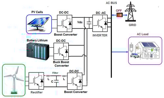
Figure 1.
Overall architecture of the proposed system.
Control is layered: conventional P–f and Q–V droop laws provide decentralized sharing, and inner voltage/current loops use PI regulators for fast tracking. The battery converter is likewise PI-controlled with mode selection driven by Vdc and SoC limits. A supervisory MPC layer (introduced later) adjusts the droop/PI setpoints rather than replacing them, enforcing converter, SoC, and bus-voltage constraints while anticipating rapid load or resource changes. This modular DC-bus topology therefore exposes clear “hook points” for predictive coordination without disturbing proven primary controllers.
2.2. Modeling the PV System with Boost Converter
The PV subsystem in this work is modeled and interfaced as shown in Figure 2. Electrically, each module is represented by the well-known single-diode equivalent: a light-generated current source in parallel with a diode and a shunt leakage path, plus a series resistance accounting for metallization and contact losses. This structure captures the strong nonlinearity of the PV I–V characteristic and its sensitivity to two external stimuli—irradiance (which scales the photogenerated current) and cell temperature (which shifts the diode voltage drop and thus the knee of the curve). Practically, these dependencies mean that the operating point of the PV array drifts continuously during the day, and any fixed operating voltage would be sub-optimal for most conditions.
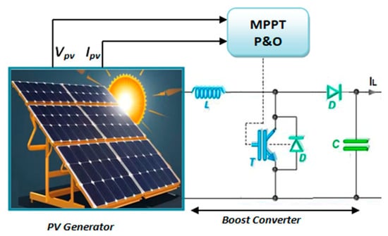
Figure 2.
The PV system circuit established in this study.
To decouple the array from the common DC bus and to force operation at the instantaneous maximum power point (MPP), the PV string feeds a unidirectional DC–DC boost converter, as shown in Figure 2. By modulating its duty cycle, this stage both elevates the array voltage to the bus level and shapes the input current seen by the panels. The converter therefore becomes the actuator through which MPPT is enforced. In this study, the boost inductor current is measured for protection and efficiency estimation, while the output capacitor maintains a low-ripple DC level for downstream converters and the VSI [43]. MPPT is implemented using the classic Perturb-and-Observe (P&O) routine because of its simplicity, low computational burden, and proven robustness in embedded environments. The decision logic, summarized in Figure 3, periodically samples the PV voltage and current, computes the instantaneous power, and compares it to the previous sample. A small perturbation (positive or negative) is injected into the reference voltage presented to the boost stage; if the measured power increases, the algorithm keeps stepping in the same direction, otherwise it reverses.
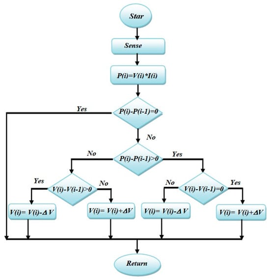
Figure 3.
Flowchart of the utilized P&O algorithm in this work.
In effect, the controller “climbs” the P–V curve until it oscillates around the true MPP. The step size and sampling period are selected to balance convergence speed and steady-state ripple; in the implementation of this work, they are also bounded by converter dynamics and sensor bandwidth. When the supervisory layer (droop/PI/MPC) demands a specific DC-bus setpoint that conflicts with unconstrained MPPT—e.g., during battery overcharge protection—the boost converter duty cycle can be clamped and the PV array temporarily curtailed. Conversely, during deficit periods the MPPT remains fully active, and the PV subsystem delivers whatever power is available, while the battery or wind branch compensates the shortfall. This coordination preserves the primary role of the PV converter—extracting maximum energy when allowed—while respecting system-wide constraints and maintaining DC-link stability.
2.3. Modeling of Battery Storage and Buck-Boost Converter
The Li-ion storage stack is represented with an equivalent-circuit model (ECM) composed of an open-circuit voltage source VOC, a lumped resistor R0, and one or more parallel R−C branches that capture diffusion and polarization dynamics, as shown in Figure 4. This structure is light enough for real-time identification yet rich enough to reproduce the rate-dependent voltage sag observed during fast charge/discharge events [44]. The slow state variable is the state of charge, updated by Coulomb counting, can be modeled as follows:
Each parallel RC leg introduces a first-order dynamic described by:
Here, the capacitor voltage Vp,n decays through its resistor when current ceases and is excited proportionally to the branch current during transients. Summing these internal voltages, adding the instantaneous ohmic drop , and superimposing the non-linear VOC (SOC) gives the measured terminal voltage, as follows:

Figure 4.
The equivalent circuit model (ECM) for battery utilized in this work.
The bidirectional energy exchange with the DC bus is handled by a non-isolated buck–boost converter, as shown in Figure 5. With switch T1 ON and T2 OFF (buck/forward mode), the inductor current charges the battery; the duty ratio d1 in (4) sets how far the output voltage Vo is stepped down from the source Vs, as follows:
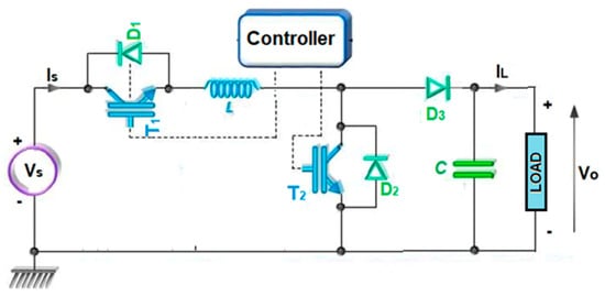
Figure 5.
The bidirectional Buck-Boost converter model with controller.
Reversing the roles—T1 OFF, T2 ON—places the converter in boost (reverse) mode, letting the battery sustain the DC bus when renewables sag; here d2 in (5) commands how aggressively Vo is lifted above Vs, as follows:
The control of this power stage follows the logic illustrated in Figure 6. A fast inner PI loop regulates either bus voltage or battery current, depending on the active mode. Above it, a simple mode-selection block monitors two signals: the DC bus voltage compared to its lower threshold and the battery SOC against its safe window. If the bus droops while SOC remains healthy, the controller asserts boost mode to support the load. If excess renewable power elevates the bus and SOC is below its upper bound, buck mode is engaged to absorb energy. Otherwise—e.g., high SOC and healthy bus—the converter relinquishes authority and higher-level droop/MPC logic throttles the sources instead.
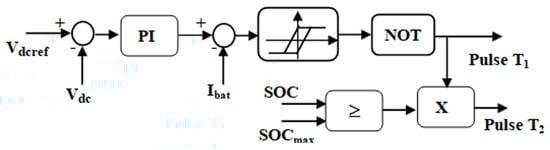
Figure 6.
An illustration of the control block of the bidirectional buck boost converter.
2.4. Modeling of the Permanent Magnet Synchronous Generator
Figure 7a condenses the complete wind-energy conversion chain adopted in this work: aerodynamic capture by a variable-pitch rotor, electromechanical transduction through a direct-drive PMSG, and dc-link conditioning via uncontrolled rectifier followed by a PWM-controlled boost stage. The upstream physics are summarized by (6)–(8):
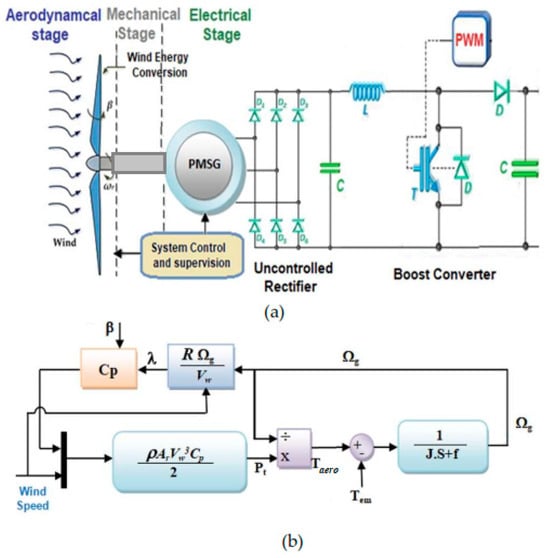
Figure 7.
The utilized model of wind turbine in this study (a) complete wind-energy conversion chain model. (b) modular block diagram of the aerodynamic and electromechanical conversion stages.
Here, is the raw kinetic power in the wind, Cp (λ, β) is the power coefficient as a function of tip-speed ratio λ and pitch angle β, and Pt is the mechanical shaft power delivered to the generator. The tip-speed ratio λ couples the rotor speed Ωg to the incoming wind velocity without the need for a gearbox, consistent with the direct-drive configuration. Figure 7b presents the modular block diagram of the aerodynamic and electromechanical conversion stages, where Cp (λ, β) feeds into the aerodynamic torque block, which in turn drives the PMSG dynamics under inertial and damping effects. The resulting electromagnetic torque provides the input for the electrical conversion stage. Finally, the empirical blade aerodynamics are represented by the polynomial in [45], mapping (λ, β) into a practical Cp surface used by the supervisory pitch controller:
With the modified tip-speed ratio defined as:
3. The Proposed Mathematical Modeling
3.1. Mathematical Description of the Distribution Feeder Operation
The proposed control strategy aims to enhance performance, stability, and operational flexibility of the hybrid renewable energy system (HRES) comprising PV, wind, and battery storage interfaced with a common DC bus and residential loads. The scheme, structured around a hierarchical control approach, integrates classical droop control with MPC. The lower-level droop control ensures immediate stability and proportional power sharing among distributed generation units, while the supervisory MPC enforces constraint satisfaction and predictive optimality over a finite horizon, particularly under variable renewable input and load conditions.
The power flow within the AC and DC domains is governed by the instantaneous power balance equations, as follows:
Equations (11) and (12) represent the active and reactive power balance, respectively, where and are the AC bus loads, is the DC-link voltage, and denotes the battery current. Equation (3) characterizes the DC-link capacitor dynamics, where denotes DC-link capacitance, critical for short-term voltage stability. It relates to the battery current measurement to the exchanged power necessary for the supervisory algorithm, as follows:
where is the converter efficiency. The battery storage dynamics are described using a simplified single-RC Thevenin equivalent circuit, as follows:
Here, Equation (15) defines the SoC, integrating the battery current over time. The transient voltage behavior under loading conditions is governed by Equations (16) and (17), involving open-circuit voltage , series resistance , and polarization dynamics characterized by a parallel resistor and capacitor. Equations (17) and (18), respectively, incorporate external environmental factors affecting PV and wind turbine outputs, such as irradiance , temperature , and wind speed . Here, the MPC treats G(t) as disturbance (forecastable), while the Droop reacts when changes suddenly. The following equations describe approximate real and reactive power flows within the distribution feeder network (, ), incorporating line impedances and , as follows:
Equations (19) and (20) guide MPC decisions by providing insight into how network power distribution responds to voltage and frequency deviations.
3.2. Mathematical Description of the PI and Droop Control Layer
The primary control layer, governed by Equations (21)–(28), is responsible for fundamental real and reactive power sharing among distributed generation units, ensuring system stability and proportional load distribution under varying conditions. First, the frequency and voltage droop characteristics, essential for decentralized operation, are defined as follows:
Here, droop coefficients and are employed to ensure proportional allocation of active and reactive power outputs, respectively. These equations establish primary operating points for frequency and voltage , based on deviations from nominal values, which serve as the basis for localized autonomous adjustments. Furthermore, distributed real and reactive power references are managed as follows:
Here, Equations (23) and (24) use weighting factors and , dynamically adjusted by the supervisory MPC, to proportionally allocate power references among converters according to their ratings. This allocation ensures effective sharing while accommodating variations in SoC or thermal limits among battery units and converters. Adaptive mechanisms are integrated within the droop control framework via:
Here, the adaptive droop gains, denoted as and , adjust control sensitivity dynamically in response to deviations in voltage and frequency from their nominal operating points. Specifically, when voltage deviations become significant, Equation (25) increases frequency sensitivity, enhancing the robustness of the frequency droop control. Conversely, significant frequency deviations trigger adjustments in voltage sensitivity via Equation (26), which improves decoupling performance under non-ideal network impedance characteristics (high R/X ratios). Further refinement of the primary layer’s operational strategy is provided by secondary set-point corrections described as follows:
Here, Equations (27) and (28) introduce slow corrective biases based on battery SoC and systematic voltage offsets. The real power reference bias in Equation (27) employs a proportional adjustment factor related to battery SoC deviation from a midpoint, enabling gradual adjustment of battery discharge or charge schedules in response to energy storage conditions. On the other hand, Equation (28) similarly provides a corrective bias for reactive power set-points using proportional factor , compensating for systematic voltage deviations and supporting optimal long-term voltage stability. Collectively, this combined droop and adaptive control approach provides foundational stability and robustness, ensuring that localized power sharing remains stable and proportional, while enabling the supervisory MPC to smoothly coordinate adjustments for enhanced overall system performance.
On the other hand, it is crucial to maintain rapid stabilization of voltage and current deviations. Hence, this work defines the inner-loop proportional-integral (PI) controllers that operate within the dq-frame, as follows:
Here, Equations (29) and (30) establish voltage errors and corresponding control actions . PI gains manage voltage deviations, correcting instantaneous errors resulting from load swings, thus ensuring immediate voltage stabilization. Similarly, Equation (31) complements the previous equations by providing decoupled q-axis voltage control, essential for independent regulation of active and reactive power components. Furthermore, Equations (32) and (33) detail the current loop PI control, where the inductor current reference tracking is managed via gains and , ensuring high-bandwidth, accurate current control within the inverter’s inner-most loop. Finally, the duty cycle commands necessary for converter modulation are determined by Equation (34), directly translating PI-controlled voltages into actionable pulse-width modulation (PWM) signals. Such a rapid-response inner loop guarantees stable and efficient converter operation, essential for interfacing RES and BESS units effectively to the distribution grid.
3.3. Mathematical Description of the MPC Layer
In this work, the supervisory MPC employs a discrete-time predictive model to forecast future system behavior and enforce optimal decision-making under dynamic operational conditions, as follows:
Here, Equation (35) establishes the state vector , incorporating key operational parameters such as voltage deviation , frequency deviation , battery state-of-charge, and battery current. Linear discrete-time state dynamics are governed by Equation (36), encapsulating the predictive evolution of system states based on control inputs and disturbance inputs , representing forecasted renewable generation and load variations. Output measurements relevant to operational constraints, directly linking observable system parameters to MPC predictions, are expressed as follows:
There is a dire need to explicitly describe critical dynamics for state evolution. Specifically, Equation (38) updates the battery SoC prediction discretely, while Equation (39) captures frequency dynamics using synthetic inertia H and damping , as follows:
Equation (40) represents approximate voltage dynamics, using an equivalent capacitance, , for reactive mismatch effects. Battery current dynamics, modeled in Equation (41), enhance MPC accuracy, particularly under constrained operational scenarios. Finally, Equation (42) defines the input control vector, encapsulating MPC-derived corrections for power set-points, facilitating precise and optimized operational adjustments. This predictive modeling framework, embedded within the MPC supervisory control structure, ensures robust constraint adherence, enhanced operational efficiency, and proactive system stability under variable renewable inputs and load conditions, as follows:
Operational constraints are critical for proper and reliable system modeling of system’s operation. Hence, the following constraints are imposed on the smart microgrid system. In specific, to ensure compliance with grid codes and system standards, voltage and frequency limits are explicitly constrained by:
Also, to prevent overcharging and deep discharge, the following battery constraints are imposed:
On the other hand, converter and battery current limitations are enforced through Equation (46), preventing thermal stress and equipment damage, whereas Equation (47) maintains inverter operation within VA rating limits, while Equation (48) safeguards DC-link voltage stability, as follows:
Smooth transition constraints are imposed via Equation (49), which limits rapid command changes to protect equipment and maintain system stability. The slack variables introduced in Equation (50) allow for soft constraint handling, ensuring feasibility while minimizing violations, as follows:
where ξ is the slack, and is penalized in the cost so constraints are “as hard as possible” but aims to never make the QP infeasible.
3.4. Mathematical Description of the Execution Law
The optimization framework is implemented to systematically minimize deviations from target operating points, while carefully managing control efforts and operational feasibility, presented as follows:
Specifically, Equation (51) formulates the MPC cost function, incorporating quadratic penalties on state deviations, control increments, and slack variable usage. Terminal cost weighting is captured by Equation (53), ensuring long-term stability through the use of a Lyapunov-based terminal constraint. Moreover, Equation (44) succinctly represents the optimization as a constrained quadratic program (QP), which is efficiently solvable in real-time. This optimization structure supports real-time operational adjustments while strictly adhering to the established system constraints detailed previously. The following define the practical implementation details for MPC command integration into the control system:
where Equation (55) aggregates the outputs of existing droop and PI control layers, creating baseline commands. MPC-derived corrective actions are introduced in Equation (56), which solves the optimization problem every supervisory cycle, typically on the order of 100 ms. Blending of MPC commands with existing control layers is managed through Equation (57), employing a dynamic scheduling factor as defined in Equation (58). This adaptive blending ensures MPC commands are smoothly integrated, avoiding abrupt operational changes. Finally, execution delays inherent in real-time computing and communication are addressed as follows:
Equation (59) shifts MPC commands temporally to align with actual system execution, while Equation (60) guarantees recursive feasibility, ensuring sustained system stability and reliable constraint adherence by appropriate terminal set χ feas and cost.
Figure 8 shows the proposed two-layer MPC strategy. The developed control system consists of two cascaded loops: the green block is a voltage control loop (VCL) and regulates output voltages , to track references , using MPC with capacitor dynamics (, while the rede block is a current control loop (CCL).
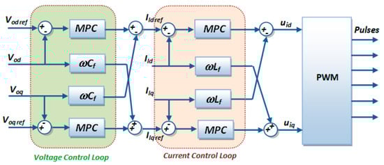
Figure 8.
Block diagram of the proposed MPC strategy.
The control scheme illustrated in Figure 8 is developed in the synchronous rotating d–q reference frame. In this frame, the three-phase AC quantities are transformed into equivalent direct-axis (d-axis) and quadrature-axis (q-axis) components, namely , for voltages and , for currents. This transformation converts sinusoidal variables into DC quantities under steady-state conditions, which significantly simplifies the design and implementation of control strategies. The voltage control loop (VCL) ensures that the output voltages track their reference values, while the current control loop (CCL) regulates the inductor currents to follow their references. By employing MPC in both loops, the system can effectively handle the cross-coupling terms (, ) between the d–q axes, achieving fast dynamic response and accurate tracking performance. Finally, the computed control signals are applied to a PWM stage to generate the switching pulses for the converter.
For PV systems, the control scheme presented in Figure 8 can be adopted. The PV array is integrated with an MPPT algorithm on the DC side of the inverter. The MPPT unit regulates the DC-link voltage to ensure maximum energy extraction from the PV source under varying irradiance and temperature conditions. At the inverter stage, the proposed MPC-based cascaded control strategy is implemented in the synchronous d–q frame. The outer voltage control loop regulates the inverter output voltages (, ) to maintain grid voltage stability, while the inner current control loop ensures accurate tracking of the inductor currents (, ). In this configuration, the d-axis current is used to control the active power delivered from the PV system, whereas the q-axis current can be adjusted to regulate reactive power or to operate at unity power factor. The computed control actions are processed through a PWM stage to generate the switching signals of the inverter, thereby enabling the PV system to deliver stable, high-quality power to the grid or local loads. A similar MPC-based cascaded control strategy, as illustrated in Figure 8, is adopted for both battery energy storage systems and wind turbines.
4. Case Study and Results
Consider a small islanded microgrid system that serve a community of buildings as depicted in Figure 9.
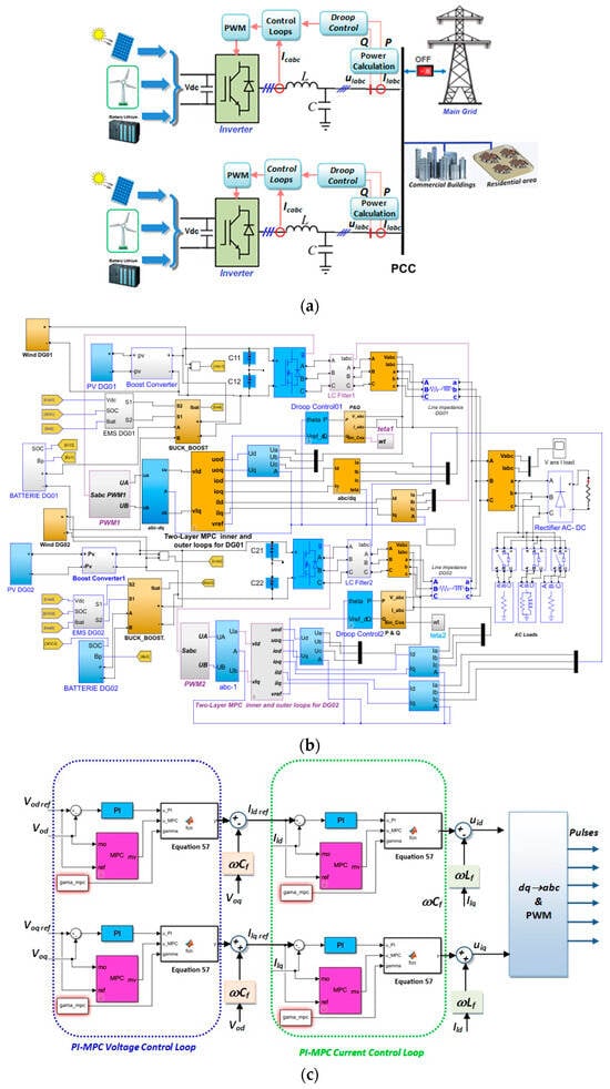
Figure 9.
Microgrid system model and architecture. (a) Conceptual/system-level block diagram with sources, control, and loads. (b) Detailed MATLAB Simulink model. (c) Proposed control structure.
The test system comprises two parallel distributed generation (DG) units interconnected via a common AC bus. Each DG unit integrates a DC link, a power electronic inverter, and an LC filter designed to ensure high-quality power delivery to the connected loads. The control architecture of each DG incorporates the proposed two-layer control algorithm, which consists of a primary droop control layer responsible for immediate autonomous response, complemented by a supervisory MPC layer that optimizes operational performance and ensures compliance with system constraints.
The generation units are characterized by distinct line impedances, emulating realistic operational scenarios. Each DG unit integrates renewable energy sources comprising 10 kW PV modules and 6 kW wind turbines, with battery storage systems serving as a distributed storage (DS) when needed. These generation and storage components are interconnected to a common DC bus via respective power electronic converters. Additionally, a 16 kW residential AC load is employed on the demand side, supported by a robust EMS designed for optimal load handling. Within the proposed control scheme, the battery storage controller plays a critical role in managing power flows within the hybrid renewable energy system, where it coordinates the charging and discharging processes, managing DC bus voltage regulation at the input of the DC/AC converter through the bidirectional DC/DC converter. This coordinated control mechanism indirectly governs the energy exchanges between power generation and storage subsystems, thereby ensuring stable and efficient microgrid operations. This test system was built in MATLAB 2023B, using an Apple MacBook with M1 pro chip, 16 GB of RAM, and a 10-core CPU.
4.1. Simulation and Initial Assessment of the Energy Management System
This subsection provides an initial assessment of the simulated microgrid system, intended for the subsequent integration of the proposed two-layer MPC-based energy management strategy. Figure 10 illustrates the solar irradiance profiles and corresponding PV generation for two solar arrays units. The irradiance varies significantly, ranging from 300 W/m2 to 1000 W/m2, representing realistic solar patterns. The PV outputs accurately track these variations, achieving peak generation levels around 6.5 kW per each of the two utilized units. In Figure 11, wind system dynamics are presented through wind speed profiles and generated wind power outputs. Wind speeds exhibit fluctuations typical of real-world conditions, with brief periods of rapid changes. The generated power profiles closely correlate with wind speed, reaching peak values near 12 kW under favorable conditions. These outcomes validate the realism of the simulated wind turbine model.
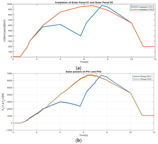
Figure 10.
Solar PV units’ performance of the test systems: (a) Irradiations, (b) Output.
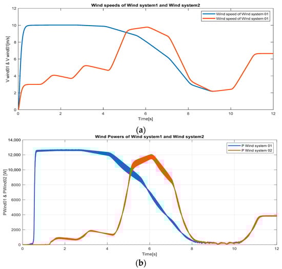
Figure 11.
Wind turbines units’ performance of the test systems: (a) Speed, (b) Output.
Similarly, Figure 12 depicts the battery storage systems’ response in terms of power and SoC. The battery systems exhibit clear transitions between charging and discharging modes, responding dynamically to the balance between renewable generation and load demands. The batteries maintain their SoC within safe operational ranges, confirming their readiness for integration with the planned MPC-based EMS.
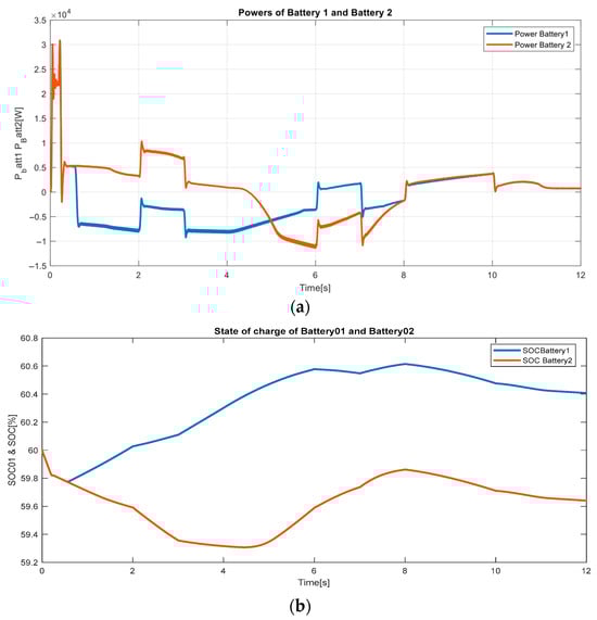
Figure 12.
Battery storage units’ performance of the test systems: (a) Power, (b) SoC.
The combined operation of the individual DG units is depicted in Figure 13. Figure 13a demonstrates the response of DG1, where wind generation initiates at around 12 kW before steadily declining after 5 s, while the solar PV power rises gradually, reaching approximately 6 kW at around 7 s, then decreases following solar irradiance reduction. Correspondingly, the battery output from DG1 dynamically adjusts within ±10 kW range, absorbing surplus generation at initial periods (0–3 s), and subsequently discharging to compensate for power deficiencies when renewable generation falls below load demands. Similarly, Figure 13b presents the operation of DG2, highlighting comparable trends but with different magnitudes owing to its distinct renewable profiles. Initially, wind generation for DG2 is relatively low (approximately 1–2 kW) and increases noticeably to peak at about 12 kW around 6 s, then rapidly diminishes. Concurrently, solar power in DG2 ramps up smoothly, peaking near 7 kW at approximately 6 s before gradually declining. The battery operation of DG2 correspondingly shows active participation, charging and discharging within a range of ±10 kW, coordinating with the renewable profiles to maintain the power balance.
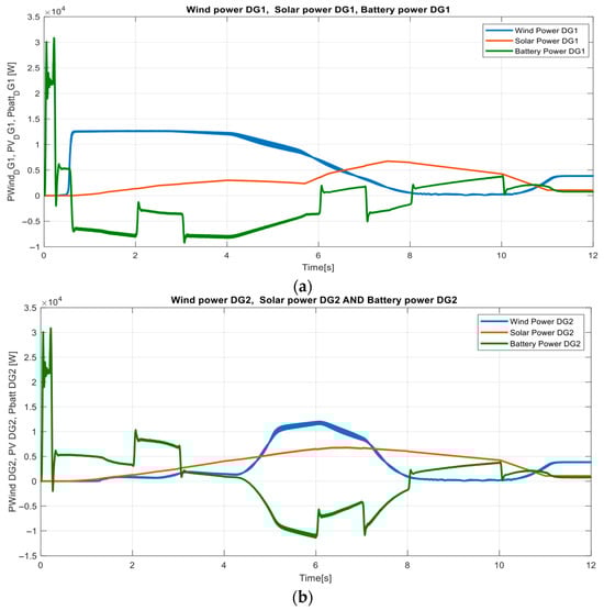
Figure 13.
Wind, PV, and Battery powers: (a) DG1, (b) DG2.
Figure 14 shows the DC-link voltage profiles of the two DG units (DG01 and DG02). Both inverters maintain a tightly regulated voltage trajectory, stabilizing around 820 V within the first 0.5 s. Figure 15 illustrates the combined contributions of wind, solar, and battery units together with the constant load demand (~15 kW). The solar generation increases steadily, reaching about 11–12 kW near 7 s before gradually declining. The total wind output remains relatively small, rising to approximately 12 kW at around 6 s and then decreasing sharply. The battery exhibits alternating charge and discharge behavior, absorbing excess energy during periods of high renewable output and supplying up to 15 kW when generation falls short. The load profile remains stepwise constant, providing a reference against which the interaction of the renewable and storage components can be observed. Despite basic balancing, transient mismatches—such as battery overcharge and undershoot—highlight the need for the proposed two-layer MPC–PI–droop control strategy introduced in the next section.
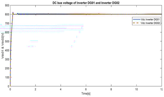
Figure 14.
DC bus voltage of inverter DG01 and inverter DG02.
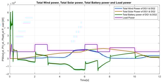
Figure 15.
Total wind power, Solar power and Battery power of DG1 and DG2.
4.2. Results of the Proposed Two-Layer Control Strategy
To examine the performance of the proposed hierarchical control system, different scenarios are considered. Table 2 summarizes the different simulation scenarios used to evaluate system performance under various loading conditions. In Scenario 1, a sudden load disturbance is introduced at t = 0.4 s to evaluate the dynamic response of the system when subjected to abrupt changes in demand. This case provides insight into the transient behavior of the system and its ability to maintain stability immediately after a disturbance. Scenario 2 examines a sequence of three different load conditions applied over the total simulation period of 12 s. From 0 to 5 s, the system is subjected to a balanced load, which serves as the baseline condition for comparison. Between 5 and 8.5 s, a non-linear load is applied to evaluate its impact on system performance, including both voltage and current harmonics. Finally, from 8.5 to 12 s, an unbalanced load is introduced to study the effects of unequal phase loading, which is a common real-world condition in distribution systems.
Table 2.
Investigated Scenarios.
4.2.1. Scenario 1
In this scenario, a sudden load disturbance was introduced at t = 0.4 s, during which the active and reactive power demands increased from 2000 W and 100 VAR to 7000 W and 2000 VAR, respectively. This disturbance persists across several steps to assess the controller’s response in real-time distributed operation. The behavior of the system is illustrated in Figure 16, Figure 17, Figure 18, Figure 19, Figure 20 and Figure 21. In Figure 16a, both inverters inject equal amounts of active power in every load scenario, with near-perfect synchronization. At every load step, the active power from each inverter rises sharply and identically, peaking around 9.5 kW in later stages. This validates the proper function of the outer droop controller, which distributes power between inverters based on a locally sensed frequency shift, and the inner PI regulator, which adjusts the inverter output to meet the droop-set references. However, it is the integration of the MPC layer that enhances the coordination further. MPC anticipates the load transitions, optimizes switching behavior, and preemptively minimizes transients. While PI and droop inherently work with local instantaneous feedback, the MPC layer considers future system states and constraints, ensuring minimal overshoot and smooth power ramping. The absence of overshoot and the symmetric, ripple-free transitions between steps are clear evidence of the MPC’s predictive regulation.
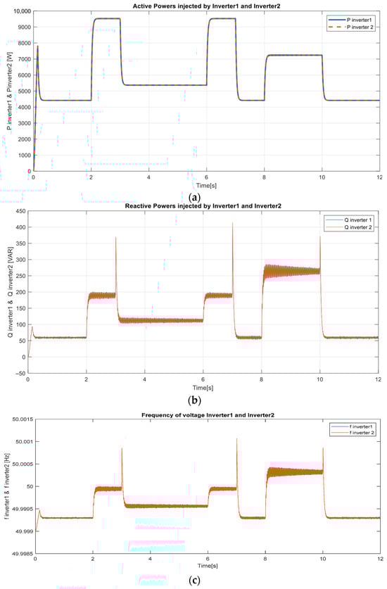
Figure 16.
Active (a), reactive (b) and frequency (c) performance of the inverters.
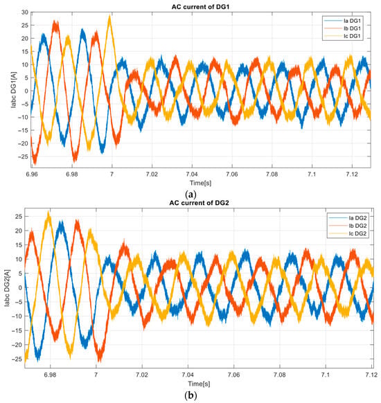
Figure 17.
AC current of (a) DG1 (b) DG2.
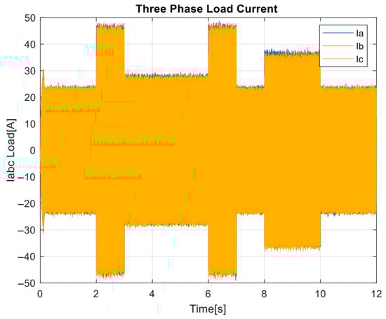
Figure 18.
Load current performance.
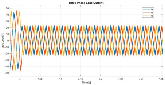
Figure 19.
A zoom-in shots of the load current.
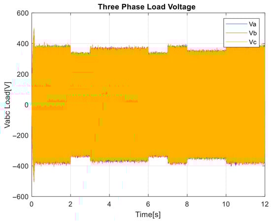
Figure 20.
3-ph load voltage performance.

Figure 21.
A zoom-in shots of the 3-ph load voltage waveform.
Similarly, Figure 16b shows balanced reactive power injection from both inverters. The system rapidly meets the 2 kVAR reactive demand with both DGs sharing equally, each contributing ~0.5 kVAR. Minor oscillations are present but contained, and again, the balanced profile reflects successful droop-based Q–V regulation supported by PI correction, while the MPC refines this further by constraining the control within system operational limits. Figure 16c reveals the frequency evolution. Despite multiple power steps, the system frequency remains stable around 50 Hz. Minor deviations do not exceed ±0.015 Hz and are quickly corrected. This fast-settling time can be attributed to the PI–droop control loop, while the smoothness and containment of transient spikes are ensured by MPC. Without MPC, these spikes would likely result in greater overshoot or undershoot, especially during simultaneous active/reactive power swings.
The quality of the current waveform injected by each inverter is shown in Figure 17. The three-phase currents of DG1 (Figure 17a) and DG2 (Figure 17b) maintain a clean, sinusoidal waveform throughout, with no distortion even at transition moments. This outcome results from the tight inner PI loop, which regulates the inverter switches at a fast timescale, while MPC supports this by adjusting reference tracking optimally over a predictive horizon. On the other hand, Figure 17 and Figure 18 confirm the corresponding behavior of the load current. The step from ~8 A to ~20–22 A per phase is handled cleanly, and the sinusoidal profile is preserved. Again, the smooth dynamic transition and waveform quality are indicative of effective current sharing and harmonic mitigation under the full control stack.
Figure 20 and Figure 21 demonstrate the performance of the proposed control strategy in maintaining the load voltage waveform. Despite abrupt changes in both active and reactive power demands, the three-phase voltage remains tightly regulated around ±310 V, exhibiting clean sinusoidal characteristics without noticeable sag, swell, or notching. This robust voltage quality results from the coordinated action of the control hierarchy: the droop controller dynamically adjusts voltage setpoints for proper load sharing, the PI controllers enforce fast regulation of voltage amplitude, and the MPC layer anticipates system variations and optimizes voltage tracking within physical constraints such as DC-link stability and power balance. The combined effect ensures high power quality and reliable voltage delivery under all operating conditions.
The results confirm that the proposed hierarchical two-layer MPC–supervised control not only achieves accurate power sharing and frequency/voltage regulation under step disturbances, but also ensures minimal transients, clean sinusoidal waveforms, and robust stability across all control levels. The MPC layer, positioned above the traditional PI and droop, plays a critical role in forecasting dynamic behavior and smoothing transitions—particularly valuable in high-variability microgrid environments.
4.2.2. Scenario 2
This scenario presents a comprehensive assessment of the system, beginning with normal balanced operation, followed by the influence of non-linear elements, and concluding with unbalanced loading. Figure 22 shows how the active and reactive load powers change under different loading conditions. In the first stage, from 0 to 5 s, the system operates with a balanced linear load, where the active power remains around 20–30 kW and the reactive power is minimal, about 100 VAR. This represents stable and ideal conditions with very little distortion. When a non-linear load is considered between 5 and 8.5 s, the active power rises sharply to nearly 45 kW, while the reactive power briefly drops toward zero and even turns slightly negative. This sudden variation demonstrates the disruptive nature of non-linear loads, which introduce significant harmonic distortion. Finally, from 8.5 to 12 s, the system experiences an unbalanced linear load. In this case, the active power decreases to about 25 kW, while the reactive power increases to nearly 2500 VAR, reflecting the uneven power flow typical of unbalanced operating conditions. Together, the figure highlights how balanced loads support stable operation, non-linear loads cause severe harmonic issues, and unbalanced loads mainly affect reactive power and voltage stability.
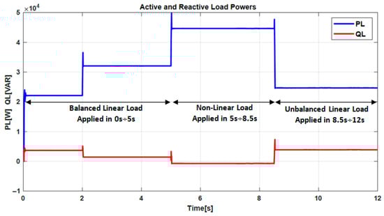
Figure 22.
Active and reactive load powers under different loading conditions: balanced linear load (0–5 s), non-linear load (5–8.5 s), and unbalanced linear load (8.5–12 s).
Figure 23 depicts the load voltage and current waveforms under different operating conditions. Figure 23a shows that the voltage waveform remains almost perfectly sinusoidal, reflecting the ability of the supply system to maintain good voltage quality even under changing load conditions. The current waveform, as shown in Figure 23b, however, provides a different observation. Under balanced loading, the current follows the voltage smoothly and maintains its sinusoidal shape. Once non-linear loads are introduced, the current becomes noticeably distorted, drifting away from the ideal waveform and revealing the presence of harmonics. In the unbalanced load case, the current waveform also loses its symmetry, which can cause uneven power sharing between phases and place stress on equipment. Together, these results make it clear that while voltage tends to remain stable, the current is much more sensitive to load type, especially under non-linear and unbalanced conditions that can harm overall power quality.
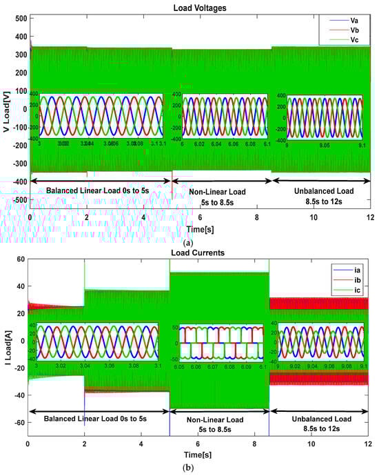
Figure 23.
Load voltage (a) and current (b) waveforms under balanced, non-linear, and unbalanced loading conditions.
In this study, the harmonic spectrum of both voltage and current was examined under three operating conditions: balanced, unbalanced, and non-linear loading. Although the unbalanced case was analyzed, its results did not reveal major differences or significant distortions when compared to the other cases. For this reason, Figure 24 and Figure 25 focus on the balanced and non-linear scenarios, where the comparison is much clearer. Figure 24 presents the harmonic spectrum analysis of the load voltage, while Figure 25 illustrates the load current.
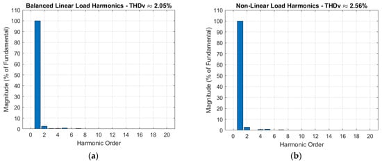
Figure 24.
Load voltage harmonic spectrums under (a) balanced and (b) non-linear loading conditions.
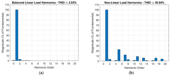
Figure 25.
Load current harmonic spectrums under (a) balanced and (b) non-linear loading conditions.
The harmonic spectrums in Figure 24 and Figure 25 illustrate the impact of balanced linear and non-linear load conditions on voltage and current waveform quality. Under the linear load, as shown in Figure 24a, the voltage harmonic spectrum is almost entirely dominated by the fundamental frequency, with only very small magnitudes at higher-order harmonics. This behavior reflects the typical characteristics of linear loads, where the current waveform closely follows the applied voltage. In contrast, as shown in Figure 24b, the non-linear load adds noticeable changes in the voltage harmonic spectrum. While the fundamental component remains dominant, additional harmonic orders—particularly the lower odd harmonics—begin to emerge. These additional components result from the use of rectifier-type loads, which distort the current and consequently affect the voltage waveform. It is evident from Figure 24 that, in terms of load voltage, linear loads tend to preserve waveform purity, whereas non-linear loads introduce additional distortion into the system. Figure 25a,b highlight the clear difference in current harmonic behavior under linear and non-linear load conditions. For the linear load, shown in Figure 25a, the current is almost entirely made up of the fundamental frequency, with only very small magnitudes at higher-order harmonics. This produces a waveform that is clean and close to an ideal sinusoid, which is reflected in the low distortion level. In contrast, Figure 25b shows how a non-linear load changes the picture. Here, several additional harmonic orders, especially the 5th, 7th, and 11th, become much more pronounced. These harmonics are typical of equipment such as rectifiers, which draw distorted, non-sinusoidal currents. As a result, the current waveform contains much higher distortion, leading to a significantly larger THD value. This comparison makes it evident that non-linear loads are a major source of harmonic pollution, while linear loads help maintain a much cleaner and more stable current waveform.
Table 3 presents a summary of the THD values for load voltages and currents under various loading conditions. The results confirm that the proposed two-layer MPC strategy maintains satisfactory power quality across different operating scenarios. For the balanced linear load, the harmonic distortion of both load voltage and current remains very low, with THD values of 2.05%. These values demonstrate good waveform quality and are consistent with the limits recommended by IEEE-519. When a non-linear load is introduced, represented by a diode-bridge rectifier with an RL branch, the voltage THD shows only a slight increase to 2.56%, but the current THD rises dramatically to 30.95%. This is a typical behavior under rectifier-type loads, where current harmonics dominate and impose additional stress on the distribution system. For the unbalanced RL load, the control scheme maintains acceptable harmonic levels, with load voltage THD reduced to 1.76% and load current THD at 1.76%. Overall, the analysis shows that the proposed control framework provides robust voltage regulation and maintains good harmonic performance for balanced and unbalanced linear loads, while still containing voltage distortion under highly non-linear conditions. The relatively high current THD observed under rectifier-type loading reflects the inherent characteristics of non-linear loads rather than controller deficiencies, but the voltage THD remains within acceptable ranges, indicating effective harmonic mitigation at the system level.
Table 3.
A summary of THD under different loading conditions.
4.3. Efficiency and Energy Loss Analysis
This section presents an analysis of the efficiency and energy losses in the proposed microgrid control scheme. As summarized in Table 4, the efficiency and energy loss distribution across different stages of the proposed control scheme indicate that most of the system operates with negligible losses, while the feeder lines dominate the overall inefficiency. The inverters, each consisting of six IGBTs, introduce minor conduction losses of about 0.005 kW, resulting in an efficiency of 99.96%. Similarly, the LC filters contribute very small damping losses of 0.0013 kW, maintaining an efficiency of nearly 99.99%. These results demonstrate that both the conversion and filtering stages are highly efficient and do not significantly affect system performance. However, the feeder lines cause substantial resistive losses of approximately 1.699 kW at 21 A, which reduce their efficiency to 90.40%.
Table 4.
Efficiency and non-switching energy losses of the microgrid across the control scheme.
Consequently, while the inverter and filter stages provide almost the entire input power, the feeder losses emerge as the primary component, accounting for nearly all of the total system losses. Therefore, the total non-switching losses within the system are 1.705 kW.
As illustrated in Table 5, the switching losses vary across the different power electronic devices within the system. When switching losses are taken into account, their contribution becomes significantly more pronounced. The inverter switching losses amount to 2.5 kW in total, while the PV, wind, and battery buck–boost converters contribute 0.667 kW, 0.300 kW, and 0.533 kW, respectively. Together, these values sum to approximately 4 kW, which is one to four orders of magnitude greater than the conduction losses and, in practice, would dominate the thermal and efficiency profile of the system. From the analysis, it is evident that while conduction and passive component losses are small, feeder resistance and switching dynamics remain critical factors. The proposed control scheme therefore plays an important role by regulating current sharing and minimizing ripple, but further optimization of switching frequency and line impedance would be necessary to improve total system efficiency in real implementations.
Table 5.
Estimated switching losses of power electronic devices.
5. Conclusions
This paper introduces and evaluates a robust two-layer control architecture de-signed to enhance power sharing, frequency regulation, and voltage stability in dis-tributed microgrid systems comprising renewable energy sources and battery storage units. The hybrid strategy merges three complementary control mechanisms: droop-based primary power sharing, PI-based voltage and current stabilization, and a supervisory MPC algorithm that enables foresighted decision-making based on system states and predicted dynamics. Through detailed modeling and simulation, the short-comings of conventional decentralized control methods—especially under dynamic loading conditions—were clearly identified. Without the proposed supervisory layer, the system demonstrated oscillations, unbalanced power allocation, and voltage fluctuations in response to sudden load increases and variable renewable input. These issues underscore the necessity of coordinated strategies capable of harmonizing local controllers with global objectives.
By integrating MPC as a higher-level optimization layer, the proposed scheme dynamically adjusts the droop coefficients and set points in response to real-time measurements and predictions of system behavior. This results in significantly improved performance, as evidenced by precise frequency regulation (±0.015 Hz), voltage stability (~311 V peak without distortion), and robust current waveform integrity—even under severe active/reactive power changes. In particular, the MPC layer mitigates the limitations of fixed droop and PI control by enforcing power balance constraints, minimizing error over prediction horizons, and adapting reference signals based on SoC, frequency, and voltage conditions. These capabilities ensure that renewable generation is utilized more effectively, battery cycling remains within safe margins, and conversion losses are reduced—key technical factors that directly support long-term system sustainability. The resulting system demonstrates not only enhanced transient response but also improved long-term power quality and energy management.
The proposed approach is readily implementable in modern embedded digital controllers, and its modular structure allows for seamless extension to more complex grid-tied or islanded microgrid applications. Such scalability is essential for sustainable energy communities, where higher renewable penetration and distributed storage must be managed reliably across diverse operating conditions. Future work may include hard-ware-in-the-loop validation, cybersecurity co-optimization, and scalability testing for larger networks with electric vehicle fleets and flexible demand-side assets.
Author Contributions
Conceptualization, S.M., T.R., T.M.A. and Y.O.A.; methodology, S.M., T.R., T.M.A. and Y.O.A.; software, S.M.; validation, T.R. and T.M.A.; formal analysis, Y.O.A. and T.M.A.; investigation, S.M., T.R., T.M.A. and Y.O.A.; resources, T.R.; data curation, T.R. and T.M.A.; writing—original draft preparation, T.M.A., T.R. and Y.O.A.; writing—review and editing, T.M.A.; visualization, T.R.; supervision, T.M.A.; project administration, T.R. and T.M.A.; funding acquisition, T.R. and T.M.A. All authors have read and agreed to the published version of the manuscript.
Funding
The Funding of this article refer to acknowledgment.
Institutional Review Board Statement
Not applicable.
Informed Consent Statement
Not applicable.
Data Availability Statement
Data will be made available upon request.
Acknowledgments
This scientific paper is derived from a research grant funded by Taibah University, Madinah, Kingdom of Saudi Arabia—with grant number (447-13-1046).
Conflicts of Interest
The authors declare no conflicts of interest.
References
- Mohd, A.; Ortjohann, E.; Schmelter, A.; Hamsic, N.; Morton, D. Challenges in Integrating Distributed Energy Storage Systems into Future Smart Grid. In Proceedings of the 2008 IEEE International Symposium on Industrial Electronics, Cambridge, UK, 30 June–2 July 2008; pp. 1627–1632. [Google Scholar]
- Momoh, A.J. Smart Grid Design for Efficient and Flexible Power Networks Operation and Control. In Proceedings of the 2009 IEEE/PES Power Systems Conference and Exposition, Seattle, WA, USA, 15–18 March 2009; pp. 1–8. [Google Scholar]
- Bajaj, M.; Singh, K.A. Grid Integrated Renewable DG Systems: A Review of Power Quality Challenges and State-of-the-art Mitigation Techniques. Int. J. Energy Res. 2020, 44, 26–69. [Google Scholar] [CrossRef]
- Petinrin, O.J.; Shaabanb, M. Impact of Renewable Generation on Voltage Control in Distribution Systems. Renew. Sustain. Energy Rev. 2016, 65, 770–783. [Google Scholar] [CrossRef]
- Serban, I.; Teodorescu, R.; Marinescu, C. Energy Storage Systems Impact on the Short-term Frequency Stability of Distributed Autonomous Microgrids, an Analysis Using Aggregate Models. IET Renew. Power Gener. 2013, 7, 531–539. [Google Scholar] [CrossRef]
- Kim, Y.S.; Kim, E.S.; Moon, S.I. Frequency and Voltage Control Strategy of Standalone Microgrids with High Penetration of Intermittent Renewable Generation Systems. IEEE Trans. Power Syst. 2015, 31, 718–728. [Google Scholar] [CrossRef]
- Aljohani, T.M. Multilayer Iterative Stochastic Dynamic Programming for Optimal Energy Management of Residential Loads with Electric Vehicles. Int. J. Energy Res. 2024, 2024, 6842580. [Google Scholar] [CrossRef]
- Palensky, P.; Dietrich, D. Demand Side Management: Demand Response, Intelligent Energy Systems, and Smart Loads. IEEE Trans. Ind. Inf. 2011, 7, 381–388. [Google Scholar] [CrossRef]
- Torriti, J. Price-Based Demand Side Management: Assessing the Impacts of Time-of-Use Tariffs on Residential Electricity Demand and Peak Shifting in Northern Italy. Energy 2012, 44, 576–583. [Google Scholar] [CrossRef]
- Werminski, S.; Jarnut, M.; Benysek, G.; Bojarski, J. Demand Side Management Using DADR Automation in the Peak Load Reduction. Renew. Sustain. Energy Rev. 2017, 67, 998–1007. [Google Scholar] [CrossRef]
- Shewale, A.; Mokhade, A.; Funde, N.; Bokde, N.D. A Survey of Efficient Demand-Side Management Techniques for the Residential Appliance Scheduling Problem in Smart Homes. Energies 2022, 15, 2863. [Google Scholar] [CrossRef]
- Said, D. A Survey on Information Communication Technologies in Modern Demand-Side Management for Smart Grids: Challenges, Solutions, and Opportunities. IEEE Eng. Manag. Rev. 2022, 51, 76–107. [Google Scholar] [CrossRef]
- De Vizia, C.; Patti, E.; Macii, E.; Bottaccioli, L. A User-Centric View of a Demand Side Management Program: From Surveys to Simulation and Analysis. IEEE Syst. J. 2022, 16, 1885–1896. [Google Scholar] [CrossRef]
- Martinez, S.; Vellei, M.; Le Dréau, J. Demand-Side Flexibility in a Residential District: What Are the Main Sources of Uncertainty? Energy Build. 2022, 255, 111595. [Google Scholar] [CrossRef]
- Kanakadhurga, D.; Prabaharan, N. Demand Side Management in Microgrid: A Critical Review of Key Issues and Recent Trends. Renew. Sustain. Energy Rev. 2022, 156, 111915. [Google Scholar] [CrossRef]
- Aljohani, T.M.; Ebrahim, A.F.; Mohammed, O. Hybrid Microgrid Energy Management and Control Based on Metaheuristic-Driven Vector-Decoupled Algorithm Considering Intermittent Renewable Sources and Electric Vehicles Charging Lot. Energies 2020, 13, 3423. [Google Scholar] [CrossRef]
- Tayab, U.B.; Roslan, M.A.; Hwai, L.J.; Kashif, M. A Review of Droop Control Techniques for Microgrid. Renew. Sustain. Energy Rev. 2017, 76, 717–727. [Google Scholar] [CrossRef]
- Firmansyah, R.; Ramli, M.A. A New Adaptive Droop Control Strategy for Improved Power Sharing Accuracy and Voltage Restoration in a DC Microgrid. Ain Shams Eng. J. 2024, 15, 102899. [Google Scholar] [CrossRef]
- Zhu, Y.; Wang, F.; Lin, Z.; Fleming, J.; Shi, T.; Guo, H.; Xu, H. Impedance Shaping Method for System-Level Stabilization of Droop-Controlled DC Microgrids. IEEE Trans. Energy Convers. 2024, 40, 409–421. [Google Scholar] [CrossRef]
- Khan, M.H.; Zulkifli, S.A.; Tutkun, N.; Ekmekci, I.; Burgio, A. Decentralized Virtual Impedance Control for Power Sharing and Voltage Regulation in Islanded Mode with Minimized Circulating Current. Electronics 2024, 13, 2142. [Google Scholar] [CrossRef]
- Xu, Z.; Chen, F.; Chen, K.; Lu, Q. Research on Adaptive Droop Control Strategy for a Solar-Storage Dc Microgrid. Energies 2024, 17, 1454. [Google Scholar] [CrossRef]
- Aljohani, T.; Mohammed, A.M.; Mohammed, O. Tri-Level Hierarchical Coordinated Control of Large-Scale EVs Charging Based on Multi-Layer Optimization Framework. Electr. Power Syst. Res. 2024, 226, 109923. [Google Scholar] [CrossRef]
- Hu, J.; Shan, Y.; Guerrero, J.M.; Ioinovici, A.; Chan, K.W.; Rodriguez, J. Model Predictive Control of Microgrids—An Overview. Renew. Sustain. Energy Rev. 2021, 136, 110422. [Google Scholar] [CrossRef]
- Babayomi, O.; Madonski, R.; Zhang, Z.; Rodriguez, J.; Davidson, I.; Kim, D.S. Robust Model Predictive Control of Converter-Based Microgrids. IEEE Trans. Power Electron. 2025, 40, 17124–17146. [Google Scholar] [CrossRef]
- Nassereddine, K.; Turzynski, M.; Bielokha, H.; Strzelecki, R. Simulation of Energy Management System Using Model Predictive Control in AC/DC Microgrid. Sci. Rep. 2025, 15, 5388. [Google Scholar] [CrossRef] [PubMed]
- Sadiq, M.; Su, C.L.; Ali, Z.; Rouhani, S.H.; Straka, M.; Buzna, L.; Micallef, A.; Parise, G. Decentralized Model Predictive Control for Offshore Wind-Powered Seaport DC Microgrids with Electric Vehicle Stations. IEEE Trans. Ind. Appl. 2025, 61, 2258–2270. [Google Scholar] [CrossRef]
- Carnielutti, F.; Busarello, T.D.; Resende, Ê.C.; Ullah, Q.; Simões, M.G. Fixed Switching Frequency Model Predictive Control for Grid-Forming Inverters. IEEE Trans. Power Electron. 2025, 40, 9080–9089. [Google Scholar] [CrossRef]
- Nori, A.; Abdulabbas, A.; Aljohani, T.M. Coordinated Sliding Mode and Model Predictive Control for Enhanced Fault Ride-Through in DFIG Wind Turbines. Energies 2025, 18, 4017. [Google Scholar] [CrossRef]
- Li, P.; Huo, X. Simplified Finite Control Set Model Predictive Control for Single-Phase Grid-Tied Inverters with Twisted Parameters. Electr. Power Syst. Res. 2025, 238, 111063. [Google Scholar] [CrossRef]
- Zhao, Z.; Zhang, X.; Zhong, C. Model Predictive Secondary Frequency Control for Islanded Microgrid under Wind and Solar Stochastics. Electronics 2023, 12, 3972. [Google Scholar] [CrossRef]
- Ma, S.; Ding, J. Multi-Model Based MPC to Improve the Ramp Rate for Renewable Energy Consumption. Neurocomputing 2025, 611, 128619. [Google Scholar] [CrossRef]
- Kumar, K.; Bae, S. Coordinated Dynamic Power Management for Renewable Energy-Based Grid-Connected Microgrids Using Model Predictive Control. IEEE Trans. Ind. Inf. 2022, 19, 9596–9608. [Google Scholar] [CrossRef]
- Hu, S.; He, L.; Zhao, H.; Liu, H.; Liu, X.; Qiu, J. Distributed Secondary Control of Microgrids with Unknown Disturbances and Non-Linear Dynamics. Front. Energy Res. 2023, 10, 1113110. [Google Scholar] [CrossRef]
- Marín, L.G.; Sumner, M.; Muñoz-Carpintero, D.; Köbrich, D.; Pholboon, S.; Sáez, D.; Núñez, A. Hierarchical Energy Management System for Microgrid Operation Based on Robust Model Predictive Control. Energies 2019, 12, 4453. [Google Scholar] [CrossRef]
- Beus, M.; Banis, F.; Pandžić, H.; Poulsen, N.K. Three-Level Hierarchical Microgrid Control—Model Development and Laboratory Implementation. Electr. Power Syst. Res. 2020, 189, 106758. [Google Scholar] [CrossRef]
- Hans, C.A.; Braun, P.; Raisch, J.; Grune, L.; Reincke-Collon, C. Hierarchical Distributed Model Predictive Control of Interconnected Microgrids. IEEE Trans. Sustain. Energy 2019, 10, 407–416. [Google Scholar] [CrossRef]
- Dao, L.A.; Dehghani-Pilehvarani, A.; Markou, A.; Ferrarini, L. A Hierarchical Distributed Predictive Control Approach for Microgrids Energy Management. Sustain. Cities Soc. 2019, 48, 101536. [Google Scholar] [CrossRef]
- Hu, J.; Shan, Y.; Yang, Y.; Parisio, A.; Li, Y.; Amjady, N.; Islam, S.; Cheng, K.W.; Guerrero, J.M.; Rodríguez, J. Economic Model Predictive Control for Microgrid Optimization: A Review. IEEE Trans. Smart Grid 2023, 15, 472–484. [Google Scholar] [CrossRef]
- Shirsat, A.; Tang, W. Data-Driven Stochastic Model Predictive Control for DC-Coupled Residential PV-Storage Systems. IEEE Trans. Energy Convers. 2021, 36, 1435–1448. [Google Scholar] [CrossRef]
- He, P.; Zhang, Y.; Jiao, J.; Ren, W.; Zhang, J.; Long, Z. A Photovoltaic–Storage System Configuration and Operation Optimization Model Based on Model Predictive Control. Clean Energy 2025, 9, 84–98. [Google Scholar] [CrossRef]
- Wang, K.; Ye, L.; Yang, S.; Deng, Z.; Song, J.; Li, Z.; Zhao, Y. A Hierarchical Dispatch Strategy of Hybrid Energy Storage System in Internet Data Center with Model Predictive Control. Appl. Energy 2023, 331, 120414. [Google Scholar] [CrossRef]
- Garcia-Torres, F.; Zafra-Cabeza, A.; Silva, C.; Grieu, S.; Darure, T.; Estanqueiro, A. Model Predictive Control for Microgrid Functionalities: Review and Future Challenges. Energies 2021, 14, 1296. [Google Scholar] [CrossRef]
- Chalal, L.; Saadane, A.; Rachid, A. Unified Environment for Real Time Control of Hybrid Energy System Using Digital Twin and IoT Approach. Sensors 2023, 23, 5646. [Google Scholar] [CrossRef] [PubMed]
- Elmahallawy, M.; Elfouly, T.; Alouani, A.; Massoud, A.M. A Comprehensive Review of Lithium-Ion Batteries Modeling, and State of Health and Remaining Useful Lifetime Prediction. IEEE Access 2022, 10, 119040–119070. [Google Scholar] [CrossRef]
- Krim, Y.; Abbes, D.; Krim, S.; Mimouni, M.F. Intelligent Droop Control and Power Management of Active Generator for Ancillary Services under Grid Instability Using Fuzzy Logic Technology. Control Eng. Pract. 2018, 81, 215–230. [Google Scholar] [CrossRef]
Disclaimer/Publisher’s Note: The statements, opinions and data contained in all publications are solely those of the individual author(s) and contributor(s) and not of MDPI and/or the editor(s). MDPI and/or the editor(s) disclaim responsibility for any injury to people or property resulting from any ideas, methods, instructions or products referred to in the content. |
© 2025 by the authors. Licensee MDPI, Basel, Switzerland. This article is an open access article distributed under the terms and conditions of the Creative Commons Attribution (CC BY) license (https://creativecommons.org/licenses/by/4.0/).