Abstract
This study investigates the climatic dynamics of Odesa, Ukraine, by integrating over 200 years of archival meteorological records with recent observations from the Davis Vantage Pro2 weather station and advanced machine learning techniques. The results reveal a distinct warming trend since 1985, with average annual temperatures projected by a CNN–LSTM model to rise by more than 6–7 °C above the mid-20th-century baseline by 2029, indicating an exceptionally rapid regional climatic shift. Spatial analysis of the July 2024 heatwave demonstrated pronounced thermal gradients, with the strongest overheating observed inland and the moderating influence of the Black Sea reducing temperature extremes in coastal areas. Precipitation analysis (1985–2024) showed an overall statistically insignificant increase; however, the summer months exhibited drying tendencies, a trend reinforced by model forecasts. Solar radiation dynamics (2012–2024) highlighted significant local variability shaped primarily by atmospheric conditions rather than solar activity, with notable monthly increases in October, November, and February. The novelty of this research lies in combining long-term datasets with deep learning methods to produce localized climate scenarios for Odesa, offering new insights into the city’s transition toward extreme warming, shifting precipitation patterns, and evolving solar energy potential. The findings have direct implications for environmental modeling, energy efficiency, and the development of climate change adaptation strategies in urbanized coastal regions.
1. Introduction
Climate change, combined with rapid urbanization, poses a significant threat to human societies [1]. Urbanization intensifies local warming through changes in land use, industrial activity, high energy consumption [2,3,4], and the expansion of impervious surfaces such as asphalt and concrete [5]. High building density, heavy traffic, and limited green spaces contribute to the formation of urban heat islands [6,7,8], where temperatures in cities can be several degrees Celsius higher than in surrounding rural areas, particularly at night [9,10,11]. Extreme weather events, including increased rainfall intensity, lead to a higher likelihood of local flooding in cities with inefficient drainage systems. Elevated temperatures also increase energy demand, greenhouse gas emissions, and the formation of photochemical smog, especially in summer [12,13,14,15]. In 2024, more than 4.61 billion people—approximately 57% of the global population—lived in urban areas [16]. The UN projects that by 2050, this share will rise to 68%, further complicating the implementation of climate adaptation strategies. Long-term studies, such as those conducted in central urban areas of China, show that over the past 40 years, the average temperature has risen by 1.58 °C, of which about 0.01 °C is attributed to urban expansion and 0.09 °C to the temperature increase in the most densely urbanized zones [17,18]. To mitigate these impacts, cities are increasingly adopting measures such as green roofs and walls, reflective building materials, improved urban planning to enhance ventilation, and sustainable transportation systems [19].
The Ministry of Environmental Protection and Natural Resources of Ukraine reports that since the beginning of the 20th century, the country’s average annual temperature has increased by more than 2 °C, of which 1.2 °C occurred over the past 30 years [20]. Ukraine has committed to reducing greenhouse gas emissions by 65% by 2030 compared to 1990 levels, in line with its national contribution to the Paris Agreement. This strategy requires a deeper understanding of local climate processes and the implementation of effective mitigation and adaptation measures. Southern regions remain particularly vulnerable, where military operations have led to significant disruption of the natural and ecological balance. Deforestation, air pollution, and soil degradation significantly weaken the ability of these territories to mitigate the effects of climate change. Large-scale fires in oil refineries, ammunition detonations, heavy equipment movement, and active use of aviation have caused greenhouse gas emissions and a decline in the soil’s ability to sequester carbon dioxide, absorb, and accumulate heat [21].
The climate is shaped by interrelated factors that are specific to each region of Ukraine. These are primarily solar radiation, atmospheric circulation, and precipitation. The interaction of these factors, their intensity, and the specifics of their impact are characterized by a certain territorial distinctiveness. According to the author [22], the climate in Ukraine will undergo drastic changes as a result of global warming, especially in the southern regions [22,23]. Therefore, the sustainable socio-economic development of the country requires forecasting both the state of the climate system as a whole and the dynamic changes in climate resources.
Studies of monthly precipitation dynamics in the southern regions of Ukraine in the 20th century have revealed the spatial and temporal distribution of annual precipitation during warm and cold periods based on a comparison of long-term precipitation calculated for different averaging periods. The authors’ research [24] showed that changes in the spatial and temporal distribution of temperature and precipitation in Odesa tend to increase humidity in the winter months, especially in December and January, and decrease precipitation in February. July remains the wettest month of the year. Analysis of the statistical structure (trends and periodic components) of the obtained time series allowed for the prediction of future trends in the studied areas until 2025–2030 throughout the territory of southern Ukraine [25]. Thus, in December and February, monthly precipitation is expected to be lower than at the beginning of the 21st century, and in January, precipitation is expected to be within the long-term range (15–45 mm).
Heat waves can directly affect the morbidity of city dwellers, causing heat exhaustion and heat stroke with fatal or non-fatal consequences. The indirect impact of heat waves results from an increased risk of death from various chronic diseases, primarily cardiovascular diseases [26]. Heat waves and sudden temperature increases can reduce productivity and learning ability, cognitive abilities, lead to pregnancy complications, and generally increase mortality [27]. The port city of Odesa, located on the Black Sea in southern Ukraine, is characterized by a combination of maritime and continental climates. The sea breeze reduces daytime overheating on the coast, but at the same time increases humidity, which, combined with urbanization factors, creates conditions for heat waves and sudden rainfall. The environmental conditions of the city depend not only on precipitation in the Odesa region. Changes in precipitation in the Dniester basin and the flow regime resulting from natural (minimum and maximum flow) and artificial regulation of the Dniester cascade in hydroelectric power plants also play an important role [28].
The presented studies focus mainly on the analysis of atmospheric precipitation, while the dynamics of solar radiation, temperature, wind, and their impact on the microclimate of Odesa have not been sufficiently studied. In the context of a detailed discussion of the dynamics of heat waves in the central regions of Ukraine [22,23,29], the specifics of heat waves in Odesa and its surroundings have not been studied. In general, as the above data show, it is extremely important to study the natural factors of urbanized areas that influence the formation of climate indicators.
The assessment of climate variability in urban areas is based on changes in time series of temperature, precipitation, and solar radiation, which allows for the identification of long-term trends, critical points, and hidden relationships between meteorological variables. One of the most popular methods is the Mann–Kendall test, which effectively detects trends in climate data [27,30,31]. However, the use of raw data from the Ukrainian Hydrometeorological Center’s network of meteorological stations or the urban climate monitoring network faces a number of methodological challenges. Current practice is often limited to the analysis of a single indicator, without taking into account the interaction of factors and nonlinear effects. In recent years, state-of-the-art time series forecasting methods have increasingly shifted towards deep learning architectures. Traditional statistical models such as ARIMA and SARIMA remain widely used, but their ability to capture nonlinear and long-term dependencies is limited. Recurrent neural networks (RNNs), and, in particular, Long Short-Term Memory (LSTM) networks and Gated Recurrent Units (GRU), have been successfully applied to capture temporal dependencies in complex datasets. A hybrid CNN–LSTM model, which combines two different types of neural networks—convolutional (CNN) and recurrent (LSTM)—appears to be better suited to describe the analyzed phenomenon. These networks are used together to leverage their complementary advantages in processing sequential data, such as text analysis, speech recognition, sentiment analysis, or temporal classification of signals (e.g., EEG, sensory data, etc.). CNN is used for feature extraction, followed by LSTM for modeling the temporal dependencies of these features. CNN is a convolutional neural network consisting of the following elements: convolutional layers, activation layers, pooling layers, and dense layers at the end. CNN is used mainly for processing grid-structured data, and its main advantage is the extraction of local features using convolutional filters. LSTM, on the other hand, is a type of recurrent neural network (RNN) designed to process sequential data. It has the ability to remember long-term dependencies in sequences. LSTM is characterized by memory cells that store information from previous time steps. They consist of input, output, and forget gates. These networks are successfully used in climate change analyses [30]. For example, there are studies available in which Authors [32] proposed a hybrid model combining LSTM, GRU, Particle Swarm Optimization (PSO), and Bayesian Model Averaging (BMA) for daily temperature and humidity forecasting. LSTM and GRU were optimized using PSO, and the results were aggregated via BMA to improve forecast accuracy. In study [33], it was shown that a CNN-LSTM hybrid demonstrates significantly higher stability and accuracy in temperature forecasting compared to traditional methods. The authors note improved performance through the combined approach. Authors [34] utilized the network for temperature and humidity prediction in utility tunnels with an accuracy of over 98–99%. The results served as the basis for early warning systems and ventilation control. In study [35], the authors used a CNN to detect seasonal climate patterns in time series (temperature, humidity, precipitation), followed by LSTM to process these patterns in temporal dynamics. The results showed an MSE reduction of 18–25% compared to classical LSTM.
The aim of this article is to analyze changes in urban climate parameters through statistical analysis of time series of temperature, precipitation, wind speed, and solar radiation using Odesa as an example. The research was conducted to examine the specifics of temperature distribution in Odesa and the region during the heatwave in July 2024; to identify current trends in the main energy and climate characteristics of Odesa; and to examine the impact of solar activity on changes in climate indicators over recent years. The study used a parametric method (Student’s t-test) and a non-parametric Mann–Kendall test to assess the statistical significance of trends. A hybrid CNN (Convolutional Neural Network) + LSTM (Long Short-Term Memory) model was used to forecast average annual. The scientific novelty lies in the integrated approach to the analysis of climate parameters in an urban environment, taking into account the spatial structure of heat waves and the impact of radiation and precipitation.
2. Methods
Archival data [36] and data from the modern and high-precision Davis Vantage Pro2 weather station (Davis Instruments, Hayward, CA, USA), installed in 2012 on the roof of the main academic building of Odesa Polytechnic University by the Department of Environmental Safety and Hydraulics, were used to form a series of observations. The study period of maximum wind speed and solar energy power covers the years 2012–2024, which makes it possible to capture recent changes in parameters using accurate analyzers and exceeds the duration of the 11-year solar cycle. Such a period of observations is sufficient to identify not only short-term fluctuations but also long-term climatic trends. It includes both periods of increased and decreased solar activity, which makes the analysis more representative. In addition, a time series of more than ten years meets the minimum requirements of modern climatology for detecting statistically significant changes in meteorological parameters at the local level. To observe the course of the heat wave, the temperature was recorded simultaneously according to [37] in the locations shown in Table 1.

Table 1.
List of settlements used to observe the heat wave in 2024.
The study of climate variables for reliability is carried out using parametric and non-parametric methods [27,30,31,38].
According to the parametric method, the statistical significance of the coefficient a was tested using Student’s t-test. If ta > tcr the trend is considered statistically significant. The criterion ta was calculated using the following equation:
where
where Sx and Sy are statistical estimates of the standard deviation of this value. The tcr value, which was determined on the basis of statistical tables, depends on the significance level (α = 0.05) and the number of degrees of freedom (number of observations n). The Mann–Kendall test, which is widely used for processing meteorological and hydrological series [15,17,18,19], was used as a non-parametric method for determining statistically significant trends. To assess the significance of the trend, the S statistic was calculated using the method described in [15]:
where n is the number of observations, are the values of the observations.
Next:
If n ≥ 40, the statistic SSS can be considered asymptotic, following a normal distribution with a mean of zero and a variance determined by the following equation:
where t is the size of a given linked group, and is the sum of all linked groups in the data sample.
The standardized statistical value of the test Z is calculated by the equation:
The statistical characteristics of Z are also subject to the standard normal distribution law with a mean of zero and a variance of one [15,20]. Using the tables of the two-tailed normal distribution function with known Z statistics, we calculate the probability P [%] that the tested value shows a significant trend.
Long Short-Term Memory (LSTM) networks represent an advanced class of recurrent neural networks (RNNs) that were specifically designed to address the limitations of classical RNNs in modeling long sequences. Standard RNNs often suffer from the vanishing or exploding gradient problem, which prevents them from retaining useful information over many time steps. LSTM networks overcome this challenge by introducing a memory cell and three types of gates: input, forget, and output. These gates regulate which information should be stored, which should be discarded, and which should be passed to the next layer. In this way, LSTMs are capable of maintaining relevant information over both short and long time horizons. This makes them particularly effective for time series forecasting tasks, where the ability to capture seasonal cycles, delayed effects, and long-term trends is essential. In climate-related applications, LSTM networks can successfully learn dependencies spanning decades, which cannot be captured by simpler statistical or machine learning models.
Convolutional Neural Networks (CNNs), while originally introduced for image recognition and computer vision tasks, have demonstrated significant advantages when applied to one-dimensional sequential data. CNNs use convolutional filters that slide across the time axis to detect local temporal patterns. Each filter can be thought of as a detector for specific types of fluctuations, such as rapid increases in temperature, sudden drops in humidity, or recurring short-term cycles. By stacking multiple convolutional layers, the network can build hierarchical representations, moving from simple local variations to more abstract and complex features. Pooling layers further reduce the size of the feature maps, compressing the data while preserving the most informative patterns. This not only improves computational efficiency but also helps prevent overfitting, which is especially important when working with relatively small datasets.
When combined, CNN–LSTM hybrid architectures exploit the complementary strengths of both methods. The CNN component acts as a feature extractor that processes raw sequential data and identifies important short-term dynamics. The LSTM component then models the temporal evolution of these extracted features, learning how they interact over long periods of time. This integration enables the model to capture both local and global structures in the data. In the context of temperature and humidity forecasting, CNN–LSTM architectures can, for instance, detect short-term anomalies or fluctuations in the data (via CNN) while simultaneously accounting for multi-year trends and dependencies (via LSTM). As a result, the hybrid approach often achieves higher accuracy and stability compared to using CNN or LSTM alone. Furthermore, it provides a more flexible modeling framework that can adapt to different data granularities (daily, monthly, yearly) and to diverse types of climatic indicators.
In the proposed CNN–LSTM architecture, the data flow between the CNN and LSTM layers is structured as follows:
- Input Representation
The input data is organized as a three-dimensional tensor with shape (batch_size, timesteps, features). We used 184 years of historical data with 1 feature, the input shape is (N,180,2) where N is the number of sequences in the batch.
- 2.
- CNN Processing (1D Convolution)
The convolutional layers apply 1D kernels along the time axis to extract local temporal patterns from the feature sequences. Each kernel moves across the time dimension and processes all features simultaneously. After convolution and activation (using ReLU), MaxPooling reduces the time dimension while preserving the most significant features. Input shape is (N,184,2). After convolution with 64 filters and kernel size 3 and max pooling with pool size 2, the output shape is (N,92,64).
- 3.
- Reshape for LSTM
After pooling, each time step has 64 feature maps, and there are 92 timesteps.
So, the input to LSTM: (N,92,64)
- 4.
- LSTM Layer
The LSTM will process a sequence of length 92, with each step comprising 64 features.
If LSTM has 128 units, its output shape: (N,128)
- 5.
- Dense Layer
Final Dense layer output is (N,2).
The input data included: the year of measurement and annual values of temperature or humidity for the observation period. For humidity prediction, the observation period was 1840–2024, and the number of records in the dataset was 184. For temperature prediction, the observation period was 1820–2024, and the number of records in the dataset was 204. Before feeding into the model, the data were normalized to the interval [0, 1] using Min–Max scaling, which avoids the dominance of variables with larger numerical ranges.
For model training, the data was split into training, validation, and testing sets in an 80:10:10 ratio. Training was conducted over 300 epochs with a batch size of 16. The Mean Absolute Error (MAE) [39,40,41] metric was used to evaluate the model’s accuracy. The hyperparameters were selected through iterative tuning using the validation dataset. We started from standard values reported in the literature (e.g., ReLU activation, Adam optimizer, learning rate of 0.001) and adjusted the number of filters, LSTM units, batch size, and regularization until stable and accurate performance was achieved, as reflected by the reported MSE values. After training, the model was used for step-by-step forecasting of future temperature and humidity values over 5 years, starting from the last available observations. The forecast was performed recursively: each newly predicted value was used as part of the input for the next forecasting step.
3. Results
A heatwave, defined as a period in which the daily maximum temperature exceeds the maximum temperature norm by 5 °C for more than five consecutive days [2,26], occurred in Odesa from 10 July 2024, when the temperature exceeded the norm by 7.7 °C, to 19 July, when the temperature exceeded the norm by 6.4 °C. Data from the meteorological station in Odesa and 12 locations along the meridian profiles (9 north and 3 south of the coast) were used to assess the impact of the heatwave on the city’s temperature. The distribution of daily maximum temperatures between 10 July and 19 July 2024 is shown in Figure 1.
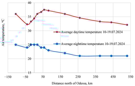
Figure 1.
Distribution of daily maximum temperatures between 10 July and 19 July 2024 in Odesa.
Data on the average annual temperature in Odesa between 1820 and 2024 [36] was used to analyze temperature changes. Trends in average annual temperatures are shown in Figure 2.
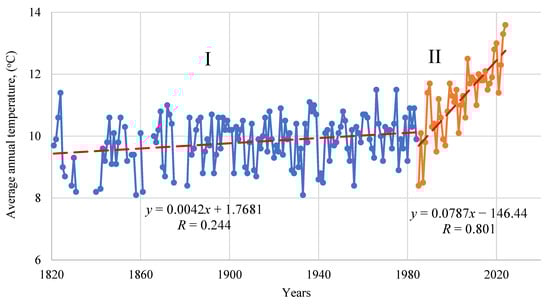
Figure 2.
Time series of average annual temperatures in Odesa.
Figure 2 presents the long-term dynamics of average annual air temperature in Odesa over the period 1820–2024, with two distinct phases clearly identified. The blue section (Zone I, 1820–1985) reflects a relatively stable climatic period, where temperature fluctuations remained within a narrow range and the linear trend indicates only a very slight increase (slope = 0.0042), with a low correlation coefficient (R = 0.244), suggesting the absence of statistically significant warming. In contrast, the orange section (Zone II, 1986–2024) demonstrates a pronounced and rapid rise in average annual temperatures, with the regression line showing a much steeper slope (0.0787) and a strong correlation (R = 0.801). This indicates the onset of a stable warming trend in the urbanized coastal environment of Odesa, consistent with global climate change tendencies. The comparison between these two phases highlights a climatic shift around the mid-1980s, marking the transition from a long-term stable thermal regime to a period of accelerated warming.
As can be seen from the changes in average annual temperatures over time, a characteristic feature of the series is a sharp increase in the parameter after 1985. For comparison, similar data [42] for the city of Kyiv for the same period were analyzed (Figure 3). The data showed similar trends in the time series.
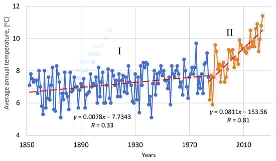
Figure 3.
Time series of average annual temperatures in Kyiv.
In order to better detect changes, the chronological series of annual average temperatures was divided into two periods: I, up to 1984; II, 1985–2024. In order to determine the statistical significance of changes in average annual temperatures and temperatures for individual months, Student’s t-test and Mann–Kendall test values were calculated separately for periods I and II using Equations (3)–(6). After calculating the Z parameter, tables were used to determine the probability P (%). If the value is negative, the trend line is downward. At a significance level (α = 0.05), the trend is statistically significant when the probability is greater than 95.0%. The calculated values for period I are presented in Table 2. The results of calculations for period II (1985–2024) are presented in Table 3. Similar calculations were performed for period II (Table 4) to determine changes in the average annual temperature in Kyiv.
Table 2.
Student’s criterion and probability of trend significance according to the Mann–Kendall test for temperature changes in Odesa for 1820–1984. Critical value of Student’s criterion tcr = 1.97.
Table 3.
Student’s criterion and probability of trend significance according to the Mann–Kendall test for temperature changes in Odesa for 1985–2024. Critical value of Student’s t-criterion tcr = 2.02.
Table 4.
Student’s criterion and probability of trend significance according to the Mann–Kendall test for temperature changes in Kyiv in 1985–2024. Critical value of Student’s t-criterion tcr = 2.02.
Trends in average annual precipitation. Changes in the amount of precipitation in Odesa are shown in Figure 4. For comparability with trends in average annual temperatures, the time series of average annual precipitation is also presented for two similar periods.
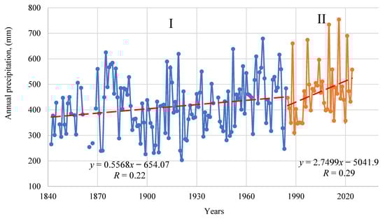
Figure 4.
Time series of annual precipitation in Odesa.
Table 5 shows the results of calculations of Student’s criterion and the Mann–Kendall test for the second chronological series of monthly precipitation for 1985–2024.
Table 5.
Student’s criterion and probability of trend significance according to the Mann–Kendall test for precipitation changes in Odesa for 1985–2024. Critical value of Student’s t-criterion tcr = 2.02.
Determining the time series of solar power received per 1 m2 of surface. The time series of solar power (Figure 5) was established based on empirical studies. The measurements were carried out using the Davis Vantage Pro2 weather station, which has been installed on the roof of the main academic building of the National University “Odesa Polytechnic” at a height of 18 m since 2012.
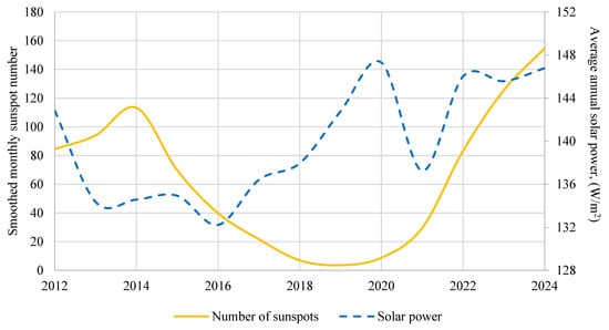
Figure 5.
Time series of solar energy power based on data from the Davis Vantage Pro2 weather station and a time series of the smoothed monthly number of sunspots according to the National Belgian Observatory (Royal Observatory, 2025 [43]).
The significance test of the trends in average annual power and for individual months is presented in Table 6.
Table 6.
Student’s criterion and probability of trend significance according to the Mann–Kendall test for changes in solar energy capacity in Odesa for 2012–2024. Critical value of Student’s criterion tcr = 2.20.
Different criteria sometimes show different directions. This is due to the different principles of constructing trend lines in these tests. Figure 6 shows the trend lines for solar power capacity for September, which have different signs. Figure 7 presents time series of annual average and maximum wind speeds in Odesa.
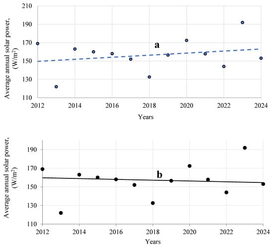
Figure 6.
Trend lines of solar energy capacity: (a) built by the least squares method; (b) built by the Mann–Kendall method.
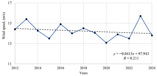
Figure 7.
Time series of annual average and maximum wind speeds in Odesa.
Figure 8 presents the results of modeling the average annual air temperature based on historical observations combined with a forecast for the next five years, obtained using a hybrid model.
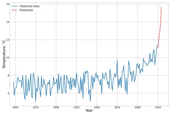
Figure 8.
Modeling of average annual air temperature using the CNN-LSTM hybrid model.
The blue line in Figure 8 shows actual data on the average annual temperature between 1850 and 2024. In the first half of this period, temperatures show relative stability with moderate interannual variability. Starting in the second half of the 20th century, and especially after the 1980s, there has been a clear upward trend in temperature, which is consistent with global climate change patterns. The red line in Figure 8 illustrates the projected values for the average annual temperature for the period 2025–2029. The projection indicates a steady and progressive increase in temperature, with an acceleration at the end of the period. The results of the temperature and humidity projections are presented in Table 7.
Table 7.
Results of the temperature and humidity forecast.
Compared to the baseline values of the mid-20th century (approximately 7–8 °C), the model predicts an increase of over 6–7 °C by the end of the decade, indicating an extremely rapid change in climatic conditions. The sharp rise in temperature at the end of the forecast period (2028–2029) may be linked to the model identifying nonlinear trends in historical data and projecting exponential growth based on accelerated changes in recent years. This scenario should be considered pessimistic or extreme, but it helps analyze potential risks to the environment, agriculture, energy systems, water supply, and human health.
Figure 9 presents the results of modeling relative humidity in combination with the forecast for the next five years.
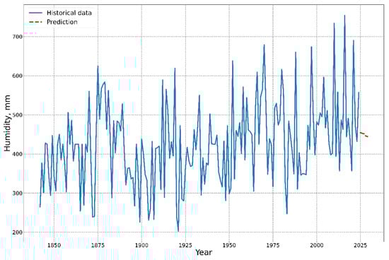
Figure 9.
Modeling of relative humidity using a hybrid CNN–LSTM model.
The blue line in Figure 9 represents historical observations of average annual humidity, while the red line shows forecasted values. According to the results, the model indicates a gradual but steady decline in humidity levels over the forecast period. If the average annual humidity in 2025 is 455 mm, it decreases to 445 mm by 2029. This suggests a potential trend toward drying or reduced precipitation.
Historical data show high variability in humidity, with numerous sharp peaks and troughs. For instance, in some years, humidity exceeded 700 mm, while in others, it fell below 300 mm. Against this backdrop, the forecasted values appear more stable, which may reflect changing climatic conditions. The decrease in precipitation could be a sign of climate change or local impacts (e.g., deforestation, urbanization, or disruptions to the water cycle). The model indicates a low likelihood of extreme precipitation in the short-term forecast, which is significant for agriculture, water resource management, and disaster prevention.
In Figure 10, the results of a comparative analysis of the Mean Squared Error for the training and validation datasets of the temperature prediction model are presented.
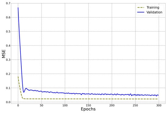
Figure 10.
Comparison of MSE values for the training and validation datasets of the temperature prediction model.
The analysis of Figure 10 indicates that the model, in general, demonstrated stable forecasting quality, despite the presence of a few individual high error values. The maximum MSE values reached 0.181 for the training dataset and 0.667 for the validation dataset, which points to the existence of certain predictions with significant deviations from the actual values. At the same time, the minimum MSE values—0.021 for the training dataset and 0.048 for the validation dataset—confirm that in the majority of cases, the model provides highly accurate results.
In Figure 11, the results of a comparative analysis of the Mean Squared Error are presented for both the training and validation datasets of the humidity prediction model.
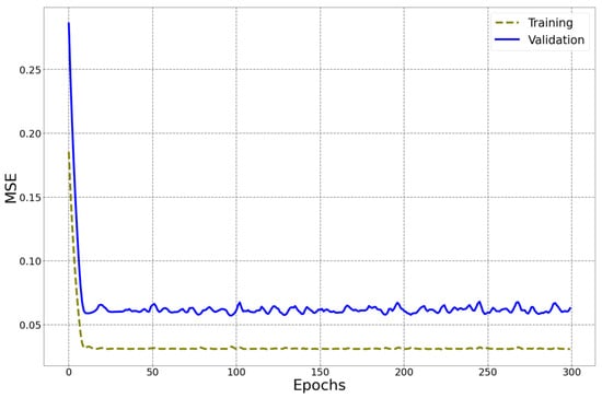
Figure 11.
Comparison of the MSE for the training and validation datasets of the humidity prediction model.
The obtained results demonstrate the overall stability of the model’s performance. This is confirmed by the relatively close MSE values observed in both datasets. Nevertheless, several isolated cases of significant error increase were detected, which led to the maximum MSE values of 0.185 for the training dataset and 0.286 for the validation dataset. These instances indicate the presence of forecasts with considerable deviations from the actual values. At the same time, the minimum MSE values—0.031 for the training dataset and 0.062 for the validation dataset—confirm the high prediction accuracy of the model in the majority of experimental cases.
The final stage of the study was testing the models using a test dataset.
Figure 12 presents the results of a comparison of actual and predicted temperatures.
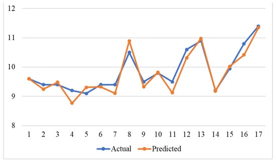
Figure 12.
Comparison of actual and predicted values of the temperature model.
Around points 4 (deviation 4.35%), 7 (deviation 3.19%), and 11 (deviation 4.21%), the prediction slightly underestimates compared to the actual values. At points 8 (deviation 3.81%) and 13 (deviation 0.92%), the model overshoots a little. At the end (points 14–17), the predicted and actual values are almost identical. The model not only matches the absolute values but also correctly follows the direction of changes—peaks, dips, and steady segments.
Figure 13 shows the results of a comparison of actual and predicted humidity.
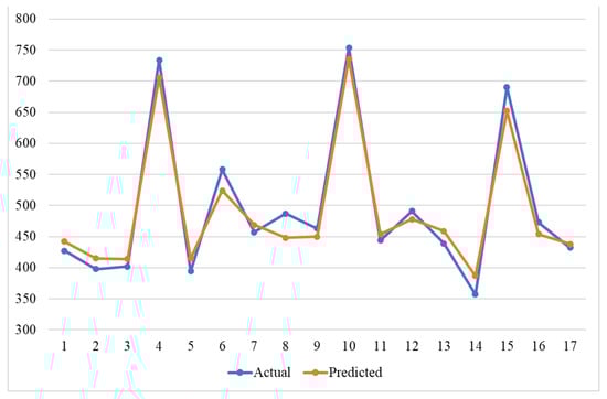
Figure 13.
Comparison of actual and predicted values of the humidity model.
The predicted values follow the actual curve very closely. The lines nearly overlap in many places, especially at stable regions (1–3, 7–9, 11–13, 16–17). At points 4 (deviation 3.96%), 10 (deviation 2.44%), and 15 (deviation 4.82%), the actual humidity shows very sharp peaks (~730–760). The model predicts these peaks slightly lower (~700–740), but still at the right positions. At points 5 (deviation 3.62%) and 14 (deviation 5.02%), the actual values dip steeply. The predicted line follows this drop well, although it tends to stay slightly above the lowest actual values (due to the slight smoothing effect).
The differences between predicted and actual values are small and systematic for both models. The model slightly underestimates high extremes and slightly overestimates the lowest dips. This behavior is typical for regression models because they minimize average error and tend to “smooth out” extremes. In summary, it can be concluded that both datasets demonstrate adequate generalization ability of the model as well as sufficient accuracy, which makes it suitable for practical applications.
4. Discussion
Cold and heat waves in recent years have significantly affected natural systems, and in urban systems, they are becoming more frequent and longer due to climate change, while at the same time being the main factor causing these changes [2,17,26]. The study showed that peak temperatures were observed 60–80 km north of Odesa (the Veliky Kuyalnyk–Berezovka area). Nighttime temperatures remain high, with a difference of only 8 °C between day and night. The greatest amplitude of daily temperature fluctuations was recorded north of the city, at a distance of 170–260 km (the Pervomaisky–Uman area). The mitigation of overheating during the day and delayed cooling at night is explained by the influence of the sea. More than 50 km south of Odesa, the temperature on the coast rose again and reached the same values as in Odesa, more than 100 km away. In this direction, the influence of southern latitudes already exceeded the influence of the sea. It was therefore concluded that sea air significantly reduces daily temperature peaks in the city, with maximum loads occurring in the north, more than 60 km from the coast. The coolest air was observed in Korolino-Buhaz in the Odesa region, even though it is located south of the city itself.
An analysis of the chronological series of annual average temperatures for the cities of Odesa and Kyiv showed a division of the series into two periods: I, up to 1985; II, 1985 to 2030. For period I, parametric and non-parametric tests (Table 2) showed a statistically significant decrease in temperature in July and an increase in temperature at the end of the year from November to December. The annual average temperatures in this period did not change significantly. In contrast, during the second period, the trends indicate an increase in the average annual temperature for all months and the year, which is consistent with global climate change patterns. In the case of Odesa, both trends were statistically significant for the entire period (Table 3). In contrast, the increase in temperature in January and February in Kyiv (Table 4) was not statistically significant. Thus, the study showed that in the second period (1985–2024), the temperature increase trend in both cities was statistically significant in all months and the year, in contrast to the previous period, when there was a decrease in summer and an increase in winter. The forecast for the average annual temperature for 2025–2029 indicates a steady and gradual increase in temperature, with an acceleration at the end of this period. The hybrid CNN and LSTM model predicts a temperature increase of more than 6–7 °C by the end of the decade, indicating an extremely rapid change in climatic conditions.
Based on an analysis of the chronological series of monthly precipitation in Odesa for the years 1985–2024 using parametric and non-parametric tests (Table 5), it was determined that, in general, there was a statistically insignificant increase in precipitation between 1985 and 2024, mainly in the cooler months. The increase in precipitation in January is statistically insignificant. On the other hand, a slight decrease in precipitation is observed in June and August (Table 5). The hybrid CNN and LSTM model predicts a slight but steady decrease in humidity levels during the forecast period. This suggests a potential trend towards drying or reduced precipitation. The data obtained are therefore consistent with the results obtained by [24,25] and show that the increase in average annual precipitation and a slight decrease in the summer months (June–August) are statistically insignificant, but the trend in the middle month of the winter season differs significantly from the trends in December and February (Table 5). The established pattern of statistical significance of temperature increase and insignificance of precipitation fluctuations is also typical for other countries, as shown in [44].
An analysis of time series of maximum wind speeds also showed no statistically significant changes. On the one hand, this indicates that there is no risk of an increase in the number of wind-induced natural disasters, and on the other hand, it allows for the expansion of wind energy designed for stable wind speeds.
Solar radiation is one of the main climate-forming factors that directly affects air temperature, evaporation, heat exchange, and the formation of local microclimates. Therefore, the analysis of time series of solar energy received per 1 m2 of surface area is crucial for understanding climate change, energy balance, and adaptation to climate change in urban areas [45]. The average recorded solar energy value in the study period is 140 W/m2, with a difference of up to 11% over the years (132.2 W/m2 in 2016 and 147.3 W/m2 in 2020). Long-term observations and statistical analysis of changes in solar radiation intensity enable, first, the identification of trends caused by changes in cloud cover, aerosol load, and air pollution. Second, these observations provide a basis for assessing the efficiency of solar energy use in the Odesa region.
In general, the observed fluctuations in solar power may coincide with changes in solar activity. However, as shown by data from the Belgian National Observatory in Figure 5, changes in solar activity during this period do not correlate with solar energy time series. Even the maximum recorded power value in 2020 corresponds to the minimum number of sunspots. The significant decrease in solar power in 2021 after an increase in 2016–2020 can be explained by the sharp, almost twofold increase in precipitation in those years, as shown in Figure 4. In terms of monthly patterns, the largest increase in solar power is observed in October–November, as well as in February (Table 6). Long-term observations and statistical analysis of changes in solar radiation intensity enable the determination of solar radiation distribution in urban areas, which is of practical importance for the development of sustainable energy, infrastructure planning, and improving the energy efficiency of buildings.
In recent works applying LSTM or hybrid CNN–LSTM models for environmental and climate-related prediction tasks, the reported MSE values typically range from 0.05 to 0.30 depending on dataset characteristics, input variables, and prediction horizons (e.g., monthly vs. yearly forecasts). For example, in the study conducted by Guo et al. [35], the obtained RMSE values were as follows: temperature forecasting: RMSE = 0.629; humidity forecasting: RMSE = 0.661. In comparison, Hou et al. [46] reported an RMSE of 1.97 for hourly temperature forecasting. Furthermore, Wu et al. [47], in their research on regional forecasts within a 1–6 h horizon, achieved an RMSE of 0.63. Finally, Zhang et al. [48] obtained an RMSE of 1.43 in the task of daily humidity forecasting. Our model achieved minimum MSE values of 0.031 (training) and 0.062 (validation), which are well within or below the lower bound of values reported in the literature, confirming the robustness of the approach.
The maximum MSE values of 0.185 (training) and 0.286 (validation) are also comparable to those reported in similar studies, especially when forecasting long-term climate indicators with inherently high variability.
The proposed CNN–LSTM architecture effectively combines local feature extraction (CNN) with long-term temporal dependencies (LSTM), leading to stable prediction performance across the datasets.
The relatively close MSE values between training and validation datasets demonstrate good generalization and limited overfitting.
The model is capable of handling long historical time series (over 180 years), which is often a challenge for classical statistical methods.
The research has some limitations. In several isolated cases, the error increased significantly, as reflected by the maximum MSE values. This indicates that the model may occasionally produce forecasts with noticeable deviations from observed data, especially in periods of abrupt climate fluctuations. Another limitation is related to data availability: only annual records of temperature and humidity were used. Additional features (e.g., CO2 concentration, solar activity, precipitation patterns) could further improve predictive accuracy. Finally, the absence of an independent external test dataset restricts the scope of validation to internal cross-validation, which, while appropriate for limited data, may not fully capture the model’s performance on unseen real-world data.
In summary, the CNN–LSTM model demonstrates competitive or superior accuracy compared with related studies, with clear strengths in stability and generalization. At the same time, we acknowledge the need for further research to address occasional high-error forecasts and to extend validation on independent datasets with richer feature sets.
5. Conclusions
This study analyzed climatic parameters of the urban environment of Odesa, including temperature, precipitation, wind speed, and solar radiation intensity, based on both long-term archival records and recent data from the Davis Vantage Pro2 weather station. The analysis of the spatial distribution of temperatures during the July 2024 heatwave using 12 meteorological stations revealed clear climatic gradients, with maximum overheating observed 60–80 km north of Odesa, while the moderating influence of the Black Sea reduced daily temperature peaks in the city itself. The smallest daily temperature amplitudes were recorded in Odesa and coastal areas, while the largest occurred in the interior of the region, highlighting the decisive role of geographical location and marine factors in shaping the local microclimate.
The chronological series of annual average temperatures in Odesa (1820–2024) showed two distinct periods: before 1985, with no statistically significant changes, and after 1985, with a pronounced increase in average annual temperatures. The results confirm stable warming in the urbanized area of Odesa, which is consistent with processes observed in Kyiv, although statistical significance differs between the two cities. Using a hybrid CNN–LSTM model, the study predicts a steady and accelerating increase in Odesa’s average annual temperature between 2025 and 2029, exceeding the mid-20th-century baseline by more than 6–7 °C by the end of the decade, indicating an extremely rapid regional climatic shift.
Analysis of precipitation dynamics (1985–2024) revealed a statistically insignificant overall increase, with only January showing a significant rise, while summer months (June and August) exhibited a decline. Forecasting with the CNN–LSTM model suggests a trend toward drier conditions or reduced precipitation, consistent with global climate tendencies of rising temperatures and relatively stable hydrometeorological parameters.
The time series of solar radiation intensity (2012–2024) recorded at the Davis Vantage Pro2 station revealed significant long-term fluctuations, with maximum values in 2020 that did not coincide with peaks in solar activity. This discrepancy indicates that local atmospheric conditions—such as cloud cover, humidity, and aerosol load—play a greater role in shaping solar energy dynamics than solar activity itself. On a monthly scale, significant increases were recorded in October, November, and February, which have practical implications for solar energy planning and building energy efficiency.
The novelty of this research lies in the combined use of long-term climatic datasets (spanning over 200 years) and advanced machine learning methods (CNN–LSTM) to detect both historical and future climatic changes in an urbanized coastal environment. Unlike previous studies, it integrates spatial analysis of heatwave gradients, intercity comparisons (Odesa vs. Kyiv), and localized solar radiation data, providing a comprehensive picture of regional climate dynamics. The CNN–LSTM model demonstrated competitive or superior forecasting accuracy (MSEmin = 0.031 training; 0.062 validation), confirming its robustness for long climate series. For the first time, localized climate scenarios for Odesa were formulated, revealing that the city is entering a stage of extremely rapid warming with distinct seasonal shifts in precipitation and solar radiation.
The results can be directly applied to environmental modeling, long-term strategic planning, and the design of climate change adaptation scenarios, thereby contributing both scientifically and practically to the understanding of urban climate transformation in coastal regions.
Author Contributions
Conceptualization. S.M., K.V., I.K. and Y.T.; methodology. S.M., K.V., I.K., D.B. and R.T.; software. S.M., K.V., I.K., D.B. and R.T.; validation. S.M., K.V., I.K., D.B. and R.T.; formal analysis. S.M., K.V., I.K. and R.T.; investigation. S.M., K.V., I.K., D.B. and R.T.; resources. S.M., K.V. and I.K.; data curation. S.M., K.V., I.K. and R.T.; writing—original draft preparation. S.M., K.V., I.K., D.B., F.C. and Y.T.; writing—review and editing. Y.T., R.T. and G.W.; visualization. Y.T.; supervision. Y.T., R.T. and G.W. All authors have read and agreed to the published version of the manuscript.
Funding
This research received no external funding.
Institutional Review Board Statement
Not applicable.
Informed Consent Statement
Not applicable.
Data Availability Statement
The original contributions presented in this study are included in the article. Further inquiries can be directed to the corresponding author.
Acknowledgments
The authors have reviewed and edited the output and take full responsibility for the content of this publication.
Conflicts of Interest
The authors declare no conflicts of interest.
References
- Das, S.; Choudhury, M.R.; Chatterjee, B.; Das, P.; Bagri, S.; Paul, D.; Bera, M.; Dutta, S. Unraveling the Urban Climate Crisis: Exploring the Nexus of Urbanization, Climate Change, and Their Impacts on the Environment and Human Well-Being—A Global Perspective. AIMS Public Health 2024, 11, 963–1001. [Google Scholar] [CrossRef]
- Vaishaly, S.; Firoz, A.B.; Sridhar, K.; Govindaraju, M. Comprehensive Analysis of Urban Heat Island and Climate Change Impact on the Environment—An Overview. Fangzhi Gaoxiao Jichukexue Xuebao 2024, 24, 326–334. [Google Scholar]
- Cheval, S.; Amihăesei, V.-A.; Chitu, Z.; Dumitrescu, A.; Falcescu, V.; Irașoc, A.; Micu, D.M.; Mihulet, E.; Ontel, I.; Paraschiv, M.-G.; et al. A Systematic Review of Urban Heat Island and Heat Waves Research (1991–2022). Clim. Risk Manag. 2024, 44, 100603. [Google Scholar] [CrossRef]
- Nuruzzaman, M. Urban Heat Island: Causes, Effects and Mitigation Measures—A Review. Int. J. Environ. Monit. Anal. 2015, 3, 67. [Google Scholar] [CrossRef]
- Debbage, N.; Shepherd, J.M. The Urban Heat Island Effect and City Contiguity. Comput. Environ. Urban Syst. 2015, 54, 181–194. [Google Scholar] [CrossRef]
- Li, D. Opportunities and Challenges for Solar Cells. Highlights Sci. Eng. Technol. 2023, 59, 129–136. [Google Scholar] [CrossRef]
- D’Agostino, D.; Congedo, P.M.; Albanese, P.M.; Rubino, A.; Baglivo, C. Impact of Climate Change on the Energy Performance of Building Envelopes and Implications on Energy Regulations across Europe. Energy 2024, 288, 129886. [Google Scholar] [CrossRef]
- Zhang, L.; Liao, W.; Chen, X.; Cheng, S.; Yang, J. Temporally Compound Heatwave and Its Interaction With Urban Heat Island Over Mainland China. Earth’s Future 2025, 13, e2025EF006490. [Google Scholar] [CrossRef]
- Li, H.; Meier, F.; Lee, X.; Chakraborty, T.; Liu, J.; Schaap, M.; Sodoudi, S. Interaction between Urban Heat Island and Urban Pollution Island during Summer in Berlin. Sci. Total Environ. 2018, 636, 818–828. [Google Scholar] [CrossRef]
- Sarrat, C.; Lemonsu, A.; Masson, V.; Guedalia, D. Impact of Urban Heat Island on Regional Atmospheric Pollution. Atmos. Environ. 2006, 40, 1743–1758. [Google Scholar] [CrossRef]
- Yang, L.; Qian, F.; Song, D.-X.; Zheng, K.-J. Research on Urban Heat-Island Effect. Procedia Eng. 2016, 169, 11–18. [Google Scholar] [CrossRef]
- Lin, H.; Li, X. The Role of Urban Green Spaces in Mitigating the Urban Heat Island Effect: A Systematic Review from the Perspective of Types and Mechanisms. Sustainability 2025, 17, 6132. [Google Scholar] [CrossRef]
- Cuce, P.M. Sustainable Insulation Technologies for Low-Carbon Buildings: From Past to Present. Sustainability 2025, 17, 5176. [Google Scholar] [CrossRef]
- Kadić, A.; Maljković, B.; Rogulj, K.; Pamuković, J.K. Green Infrastructure’s Role in Climate Change Adaptation: Summarizing the Existing Research in the Most Benefited Policy Sectors. Sustainability 2025, 17, 4178. [Google Scholar] [CrossRef]
- Mirzaei, P.A. Recent Challenges in Modeling of Urban Heat Island. Sustain. Cities Soc. 2015, 19, 200–206. [Google Scholar] [CrossRef]
- Ritchie, H.; Samborska, V.; Roser, M. Urbanization. The World Population Is Moving to Cities. Why Is Urbanization Happening and What Are the Consequences? Our World In Data. 2024. Available online: https://ourworldindata.org/urbanization (accessed on 5 July 2025).
- Shao, Q.; Sun, C.; Liu, J.; He, J.; Kuang, W.; Tao, F. Impact of Urban Expansion on Meteorological Observation Data and Overestimation to Regional Air Temperature in China. J. Geogr. Sci. 2011, 21, 994–1006. [Google Scholar] [CrossRef]
- Lynda, D.; Logeswari, G.; Tamilarasi, K.; Rakesh, S. Hybrid Bayesian Deep Learning Model for Predicting Urban Heat Island Intensity in African Cities. Sci. Rep. 2025, 15, 31280. [Google Scholar] [CrossRef]
- Bank, W. Cities and Climate Change: An Urgent Agenda. In Urban Development Series Knowledge Papers; The World Bank: Washington, DC, USA, 2010. [Google Scholar]
- Ivaniuta, S.; Kolomiiets, O.; Malynovska, O.; Yakushenko, L. Climate Change: Consequences and Adaptation Measures; NISD: Kyiv, Ukraine, 2020. [Google Scholar]
- Available online: https://zakon.rada.gov.ua/rada/show/v0386926-23#Text (accessed on 5 July 2025).
- Khokhlov, V.; Yermolenko, N. Future Climate Change and Its Impact on Precipitation and Temperature in Ukraine. Ukr. Hydrometeorol. J. 2015, 16, 76–82. [Google Scholar]
- Martazinova, V.F.; Shchehlov, O. Nature of Extreme Precipitation over Ukraine in the 21st Century. Ukr. Hydrometeorol. J. 2018, 22, 36–45. [Google Scholar] [CrossRef]
- Goncharova, L.; Prokofiev, O.; Reshetchenko, S. Features of Climate and Geographical Distribution of Atmospheric Precipitations in the South of Ukraine. Isnyk V.N. Karazin Kharkiv Natl. Univ. Ser. Geol. Geogr. Ecol. 2022, 57, 81–94. [Google Scholar] [CrossRef]
- Prokofiev, O.M.; Goncharova, L.D.; Chernyshov, V. Statistical Characteristics of Surface Wind Speed at Odesa Observatory Station and Their Dynamics in the Context of Modern Climate Change. In Proceedings of the Second International Research-to-Practice Conference, Odesa, Ukraine, 16–18 April 2025. [Google Scholar]
- Smoyer-Tomic, K.E.; Kuhn, R.; Hudson, A. Heat Wave Hazards: An Overview of Heat Wave Impacts in Canada. Nat. Hazards 2003, 28, 465–486. [Google Scholar] [CrossRef]
- Lenton, T.M.; Xu, C.; Abrams, J.F.; Ghadiali, A.; Loriani, S.; Sakschewski, B.; Zimm, C.; Ebi, K.L.; Dunn, R.R.; Svenning, J.-C.; et al. Quantifying the Human Cost of Global Warming. Nat. Sustain. 2023, 6, 1237–1247. [Google Scholar] [CrossRef]
- Melnyk, S.; Loboda, N. Trends in Monthly, Seasonal, and Annual Fluctuations in Flood Peaks for the Upper Dniester River. Meteorol. Hydrol. Water Manag. 2020, 8, 28–36. [Google Scholar] [CrossRef]
- Snizhko, S.; Shevchenko, O.; Svintsitska, H. Heat Waves in Central Regions of Ukraine Under the Conditions of Climate Change. Visnyk Taras Shevchenko Natl. Univ. Kyiv Mil.-Spec. Sci. 2018, 58–62. [Google Scholar] [CrossRef]
- Das, L.C.; Mohiul Islam, A.S.M.; Ghosh, S. Mann–Kendall Trend Detection for Precipitation and Temperature in Bangladesh. Int. J. Big Data Mini. Glob. Warm. 2022, 4, 2250001. [Google Scholar] [CrossRef]
- Salvati, L.; Zambon, I.; Pignatti, G.; Colantoni, A.; Cividino, S.; Perini, L.; Pontuale, G.; Cecchini, M. A Time-Series Analysis of Climate Variability in Urban and Agricultural Sites (Rome, Italy). Agriculture 2019, 9, 103. [Google Scholar] [CrossRef]
- Saleem, M.; Saleem, M.M.; Waseem, F.; Bashir, M.A. An Ensemble Forecasting Method Based on Optimized LSTM and GRU for Temperature and Humidity Forecasting. Eng. Technol. Appl. Sci. Res. 2024, 14, 18447–18452. [Google Scholar] [CrossRef]
- Gong, Y.; Zhang, Y.; Wang, F.; Lee, C. Deep Learning for Weather Forecasting: A CNN-LSTM Hybrid Model for Predicting Historical Temperature Data. Appl. Comput. Eng. 2024, 99, 168–174. [Google Scholar] [CrossRef]
- Peng, F.-L.; Qiao, Y.-K.; Yang, C. A LSTM-RNN Based Intelligent Control Approach for Temperature and Humidity Environment of Urban Utility Tunnels. Heliyon 2023, 9, e13182. [Google Scholar] [CrossRef]
- Guo, Q.; He, Z.; Wang, Z. Monthly Climate Prediction Using Deep Convolutional Neural Network and Long Short-Term Memory. Sci. Rep. 2024, 14, 17748. [Google Scholar] [CrossRef]
- Available online: https://meteostat.net/en/place/ua/odessa (accessed on 5 July 2025).
- Available online: https://weather.com/uk-ua/weather/today (accessed on 5 July 2025).
- Yue, S.; Pilon, P. A Comparison of the Power of the t Test, Mann-Kendall and Bootstrap Tests for Trend Detection/Une Comparaison de La Puissance Des Tests t de Student, de Mann-Kendall et Du Bootstrap Pour La Détection de Tendance. Hydrol. Sci. J. 2004, 49, 21–37. [Google Scholar] [CrossRef]
- Trach, Y.; Trach, R.; Kalenik, M.; Koda, E.; Podlasek, A. A Study of Dispersed, Thermally Activated Limestone from Ukraine for the Safe Liming of Water Using ANN Models. Energies 2021, 14, 8377. [Google Scholar] [CrossRef]
- Trach, R.; Moshynskyi, V.; Chernyshev, D.; Borysyuk, O.; Trach, Y.; Striletskyi, P.; Tyvoniuk, V. Modeling the Quantitative Assessment of the Condition of Bridge Components Made of Reinforced Concrete Using ANN. Sustainability 2022, 14, 15779. [Google Scholar] [CrossRef]
- Trach, R.; Lendo-Siwicka, M.; Pawluk, K.; Połoński, M. Analysis of direct rework costs in Ukrainian construction. Arch. Civ. Eng. 2021, 67, 397–411. [Google Scholar] [CrossRef]
- Available online: https://meteostat.net/en/station/33345 (accessed on 5 July 2025).
- Available online: https://www.sidc.be/SILSO/home (accessed on 5 July 2025).
- Xu, Z.; Tang, Y.; Connor, T.; Li, D.; Li, Y.; Liu, J. Climate Variability and Trends at a National Scale. Sci. Rep. 2017, 7, 3258. [Google Scholar] [CrossRef] [PubMed]
- Liu, H.; Li, M.; Yang, C.; Jia, L. Application of Time-Series Analysis to Urban Climate Change Assessment. Int. J. Environ. Sci. Technol. 2025, 22, 11037–11044. [Google Scholar] [CrossRef]
- Hou, J.; Wang, Y.; Zhou, J.; Tian, Q. Prediction of Hourly Air Temperature Based on CNN–LSTM. Geomat. Nat. Hazards Risk 2022, 13, 1962–1986. [Google Scholar] [CrossRef]
- Wu, S.; Fu, F.; Wang, L.; Yang, M.; Dong, S.; He, Y.; Zhang, Q.; Guo, R. Short-Term Regional Temperature Prediction Based on Deep Spatial and Temporal Networks. Atmosphere 2022, 13, 1948. [Google Scholar] [CrossRef]
- Zhang, X.; Ren, H.; Liu, J.; Zhang, Y.; Cheng, W. A Monthly Temperature Prediction Based on the CEEMDAN–BO–BiLSTM Coupled Model. Sci. Rep. 2024, 14, 808. [Google Scholar] [CrossRef] [PubMed]
Disclaimer/Publisher’s Note: The statements, opinions and data contained in all publications are solely those of the individual author(s) and contributor(s) and not of MDPI and/or the editor(s). MDPI and/or the editor(s) disclaim responsibility for any injury to people or property resulting from any ideas, methods, instructions or products referred to in the content. |
© 2025 by the authors. Licensee MDPI, Basel, Switzerland. This article is an open access article distributed under the terms and conditions of the Creative Commons Attribution (CC BY) license (https://creativecommons.org/licenses/by/4.0/).