Data-Driven Approaches for State-of-Charge Estimation in Battery Electric Vehicles Using Machine and Deep Learning Techniques


Abstract
1. Introduction
2. Related Works
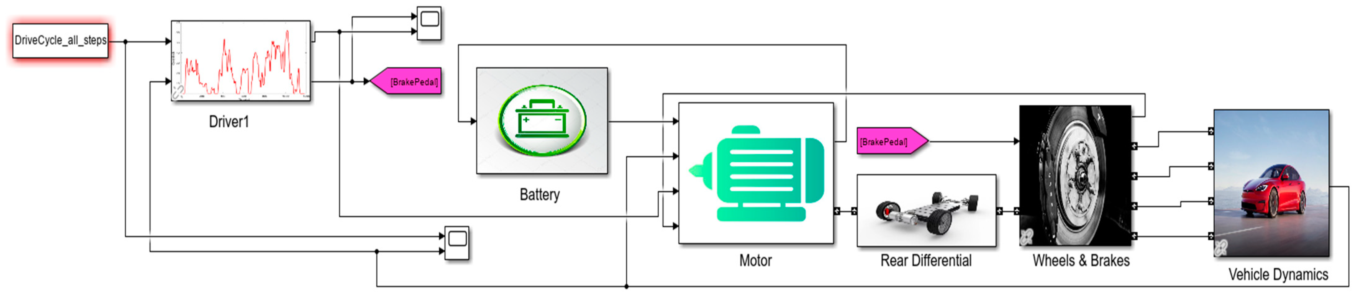
3. Model Description
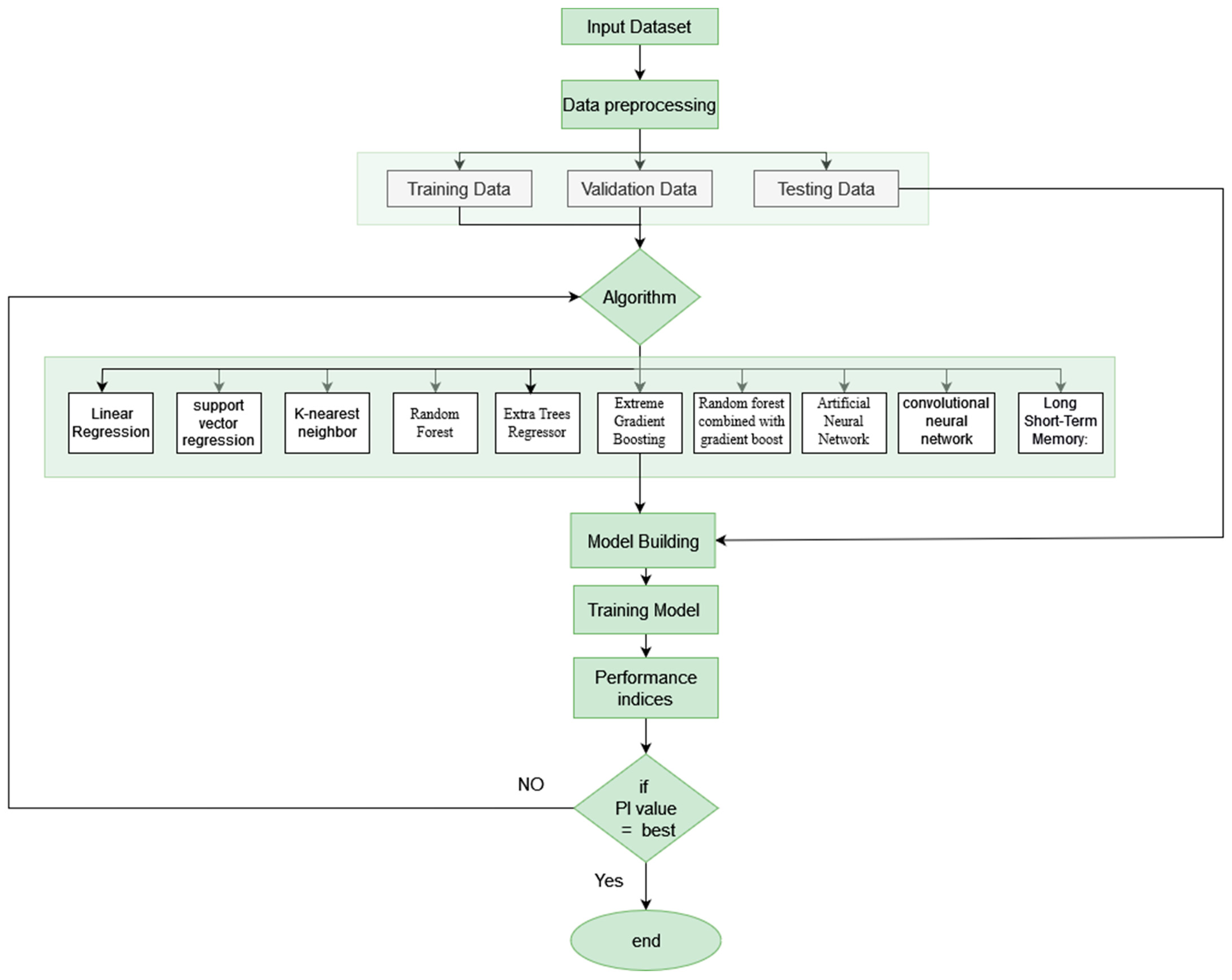
4. Machine Learning Model
4.1. Linear Regression
4.2. Support Vector Regression (SVR)
4.3. K-Nearest Neighbor (K-NN)
4.4. Random Forest
4.5. Extra Trees Regressor
4.6. Extreme Gradient Boosting
4.7. Ensemble (Random Forest Combined Gradient Boost)
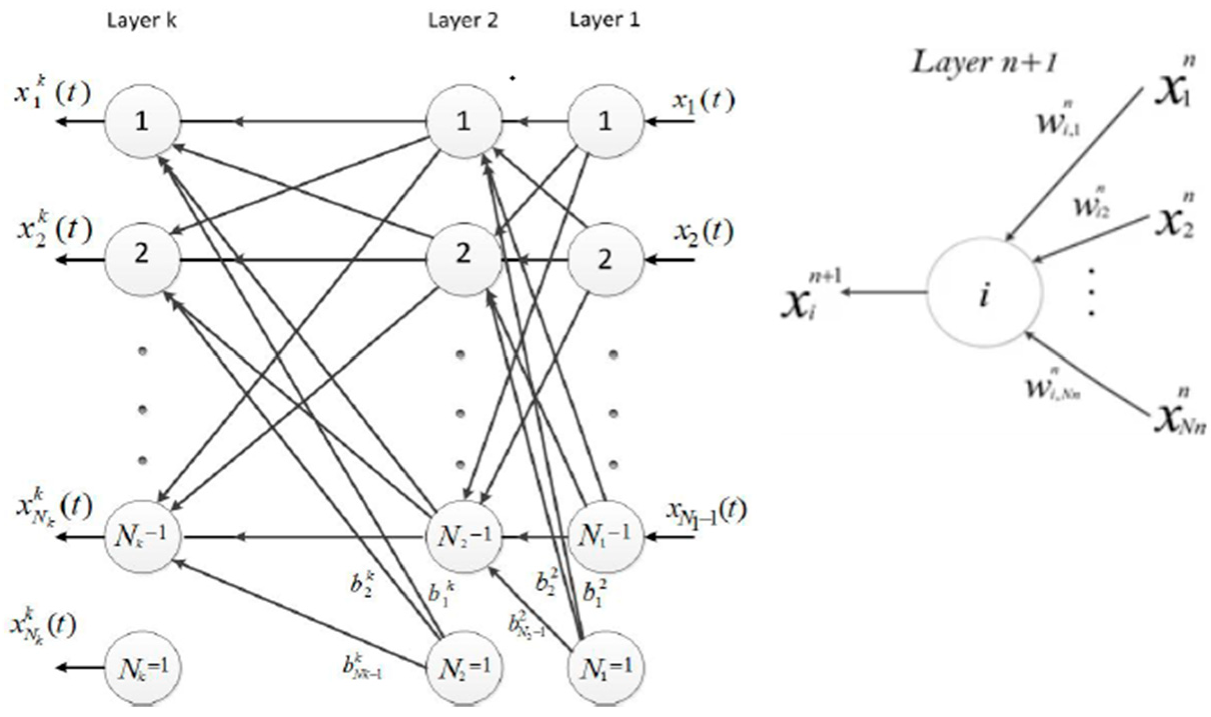
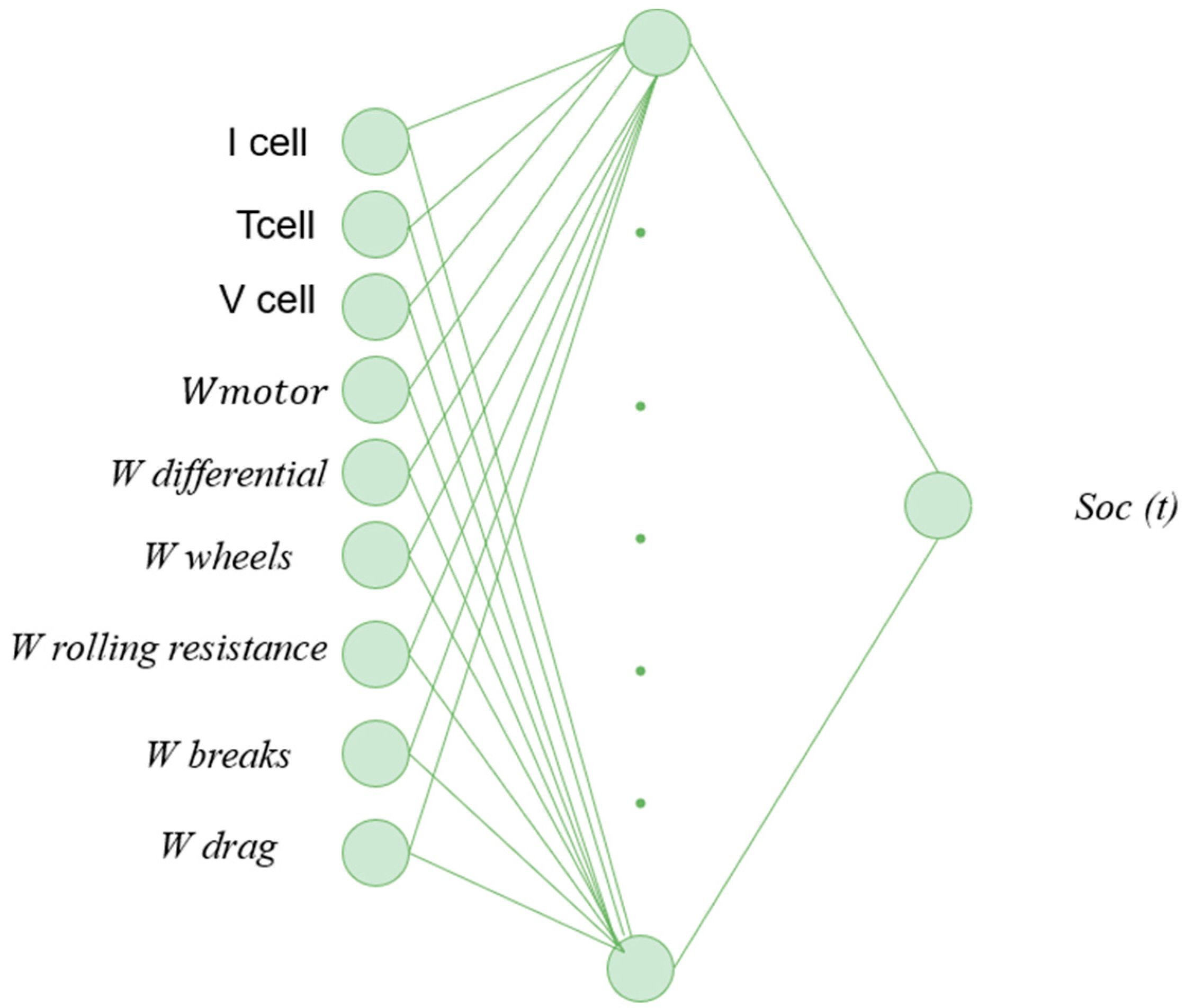
4.8. Artificial Neural Network
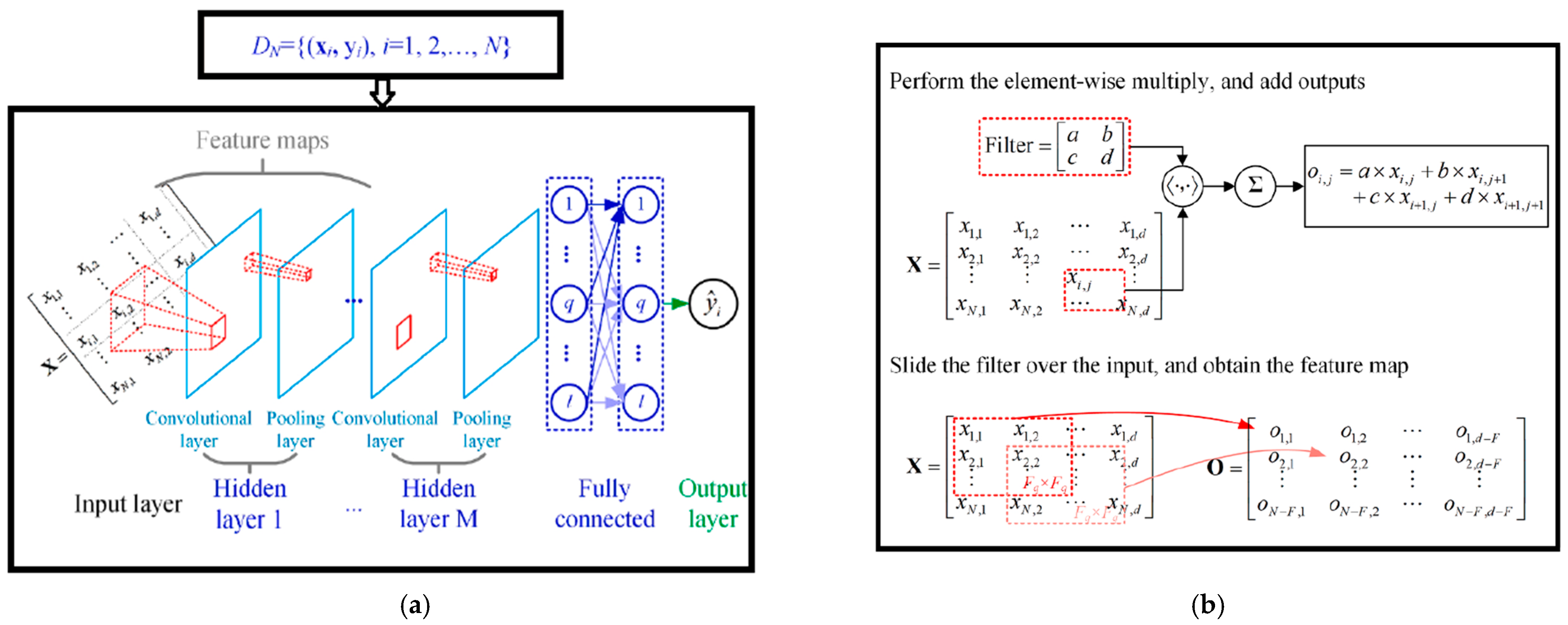
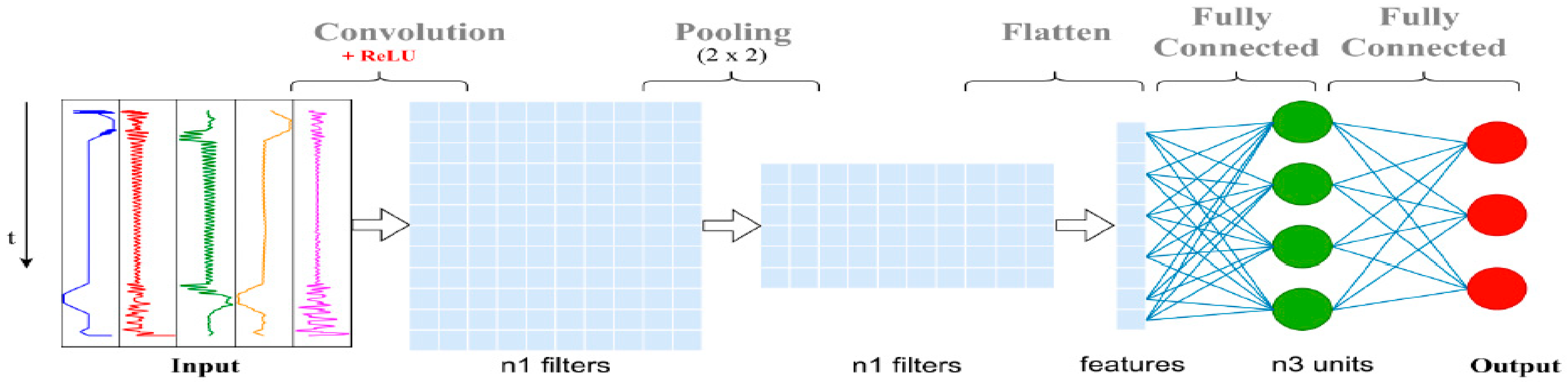
4.9. Convolutional Neural Network
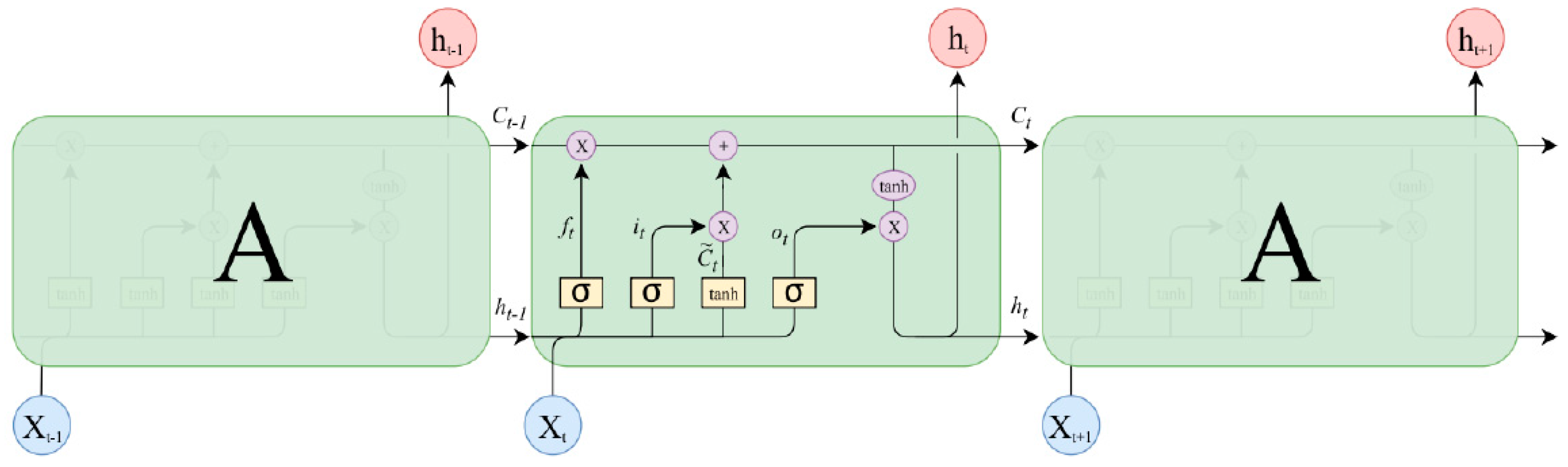
4.10. Long Short-Term Memory
5. Result and Discussion
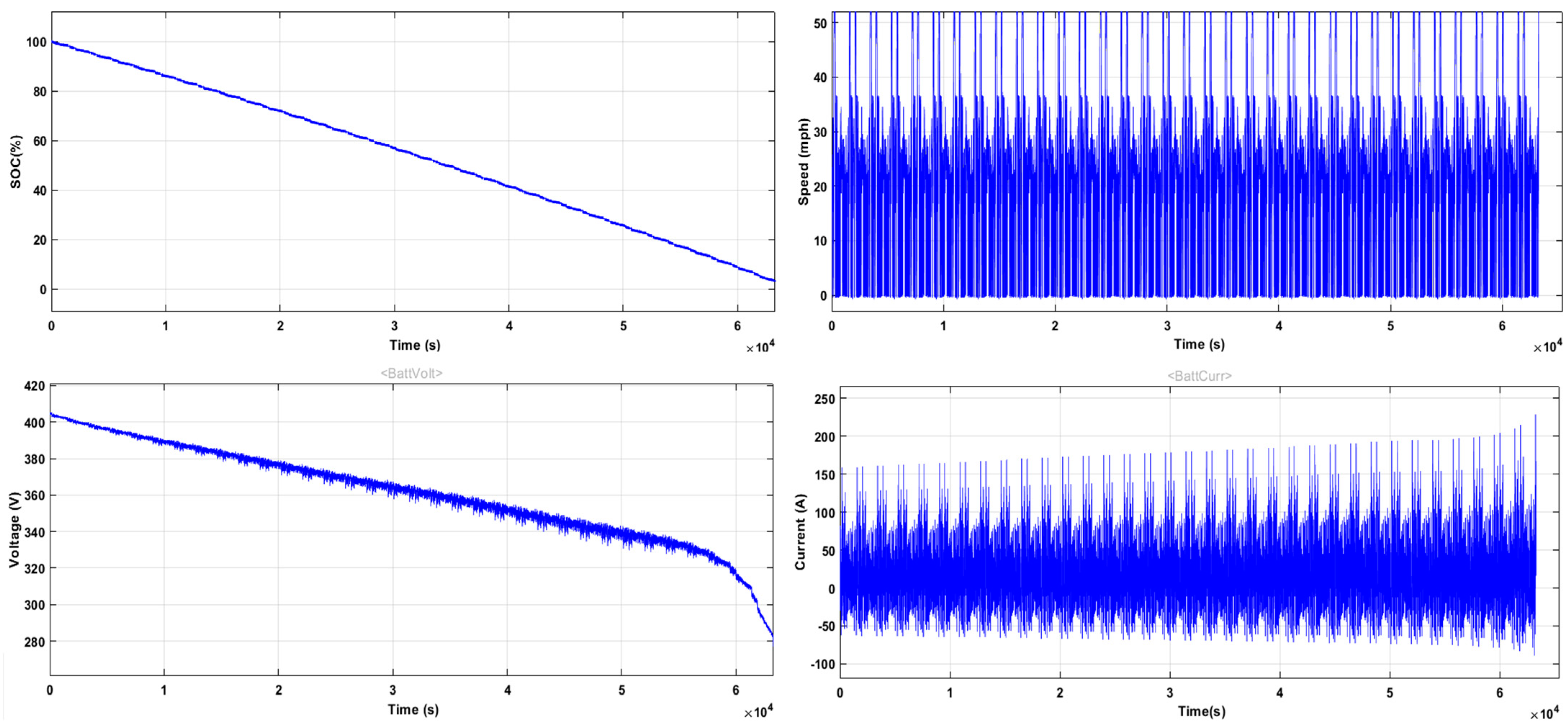
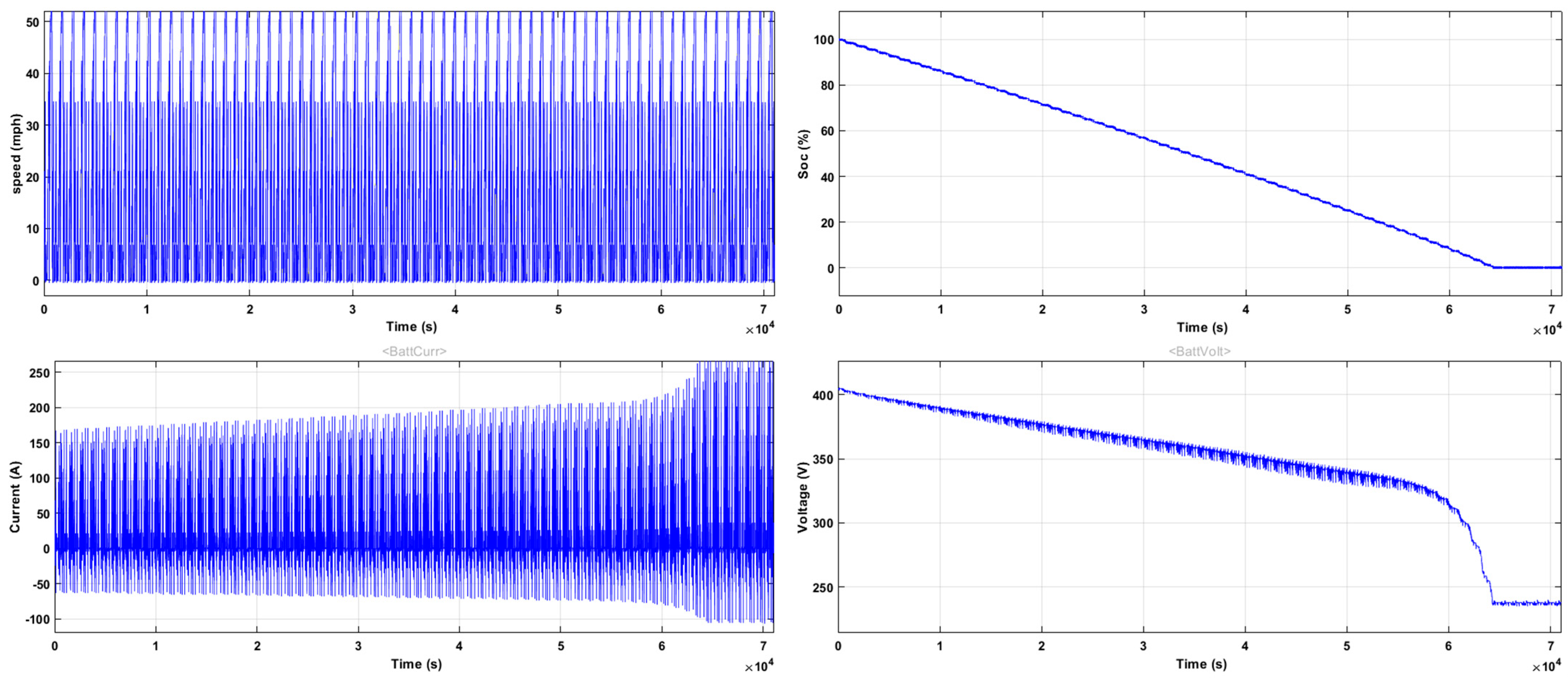
5.1. Simulations of Battery Electric Vehicles and Generation of Datasets
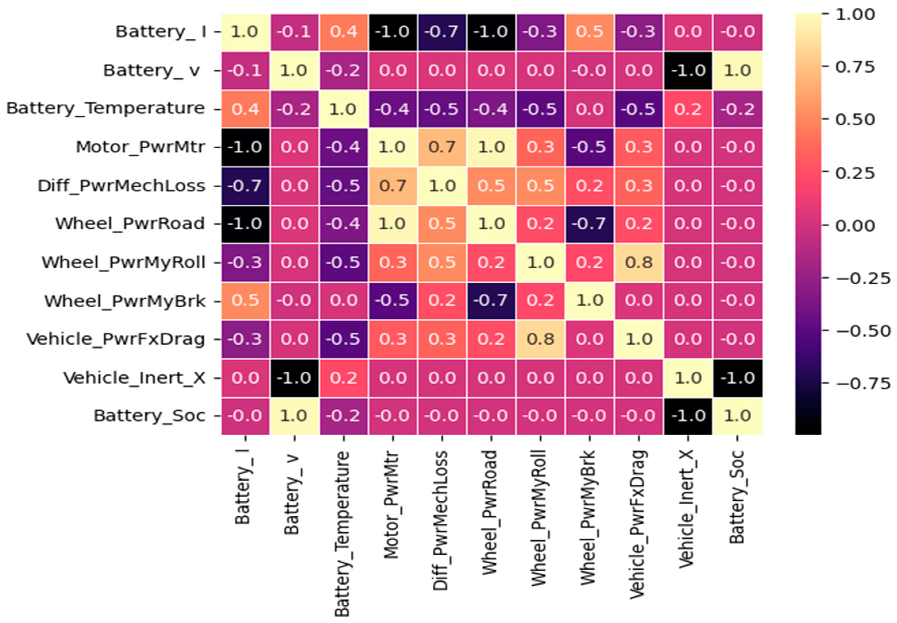
5.2. The Preparation of Data
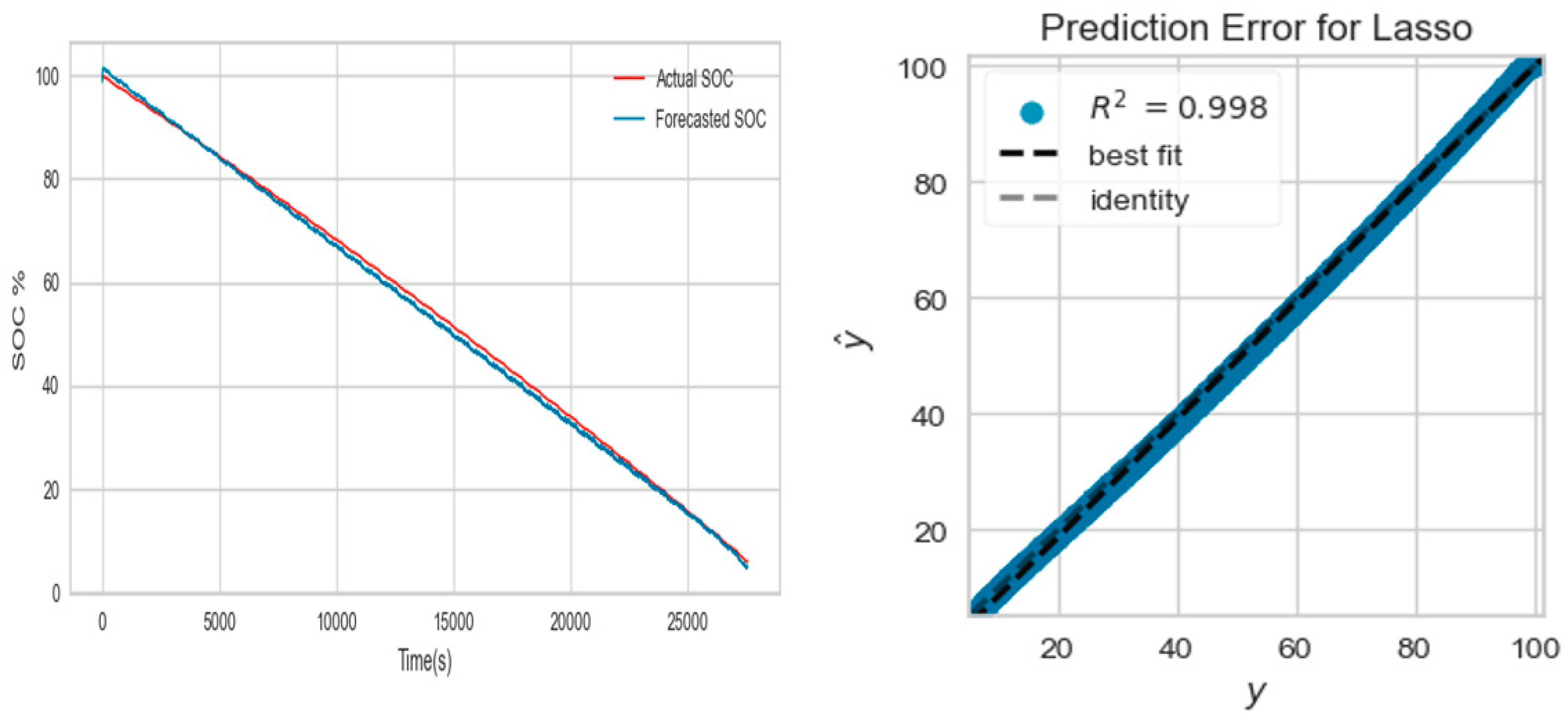
5.3. State-of-Charge Estimation Using Machine Learning Models
6. Conclusions
Author Contributions
Funding
Institutional Review Board Statement
Informed Consent Statement
Data Availability Statement
Acknowledgments
Conflicts of Interest
References
- Albrechtowicz, P. Electric vehicle impact on the environment in terms of the electric energy source—Case study. Energy Rep. 2023, 9, 3813–3821. [Google Scholar] [CrossRef]
- Sanguesa, J.A.; Torres-Sanz, V.; Garrido, P.; Martinez, F.J.; Marquez-Barja, J.M. A Review on Electric Vehicles: Technologies and Challenges. Smart Cities 2021, 4, 372–404. [Google Scholar] [CrossRef]
- Ralls, A.M.; Leong, K.; Clayton, J.; Fuelling, P.; Mercer, C.; Navarro, V.; Menezes, P.L. The Role of Lithium-Ion Batteries in the Growing Trend of Electric Vehicles. Materials 2023, 16, 6063. [Google Scholar] [CrossRef]
- Liu, W.; Placke, T.; Chau, K. Overview of batteries and battery management for electric vehicles. Energy Rep. 2022, 8, 4058–4084. [Google Scholar] [CrossRef]
- Thangavel, S.; Mohanraj, D.; Girijaprasanna, T.; Raju, S.; Dhanamjayulu, C.; Muyeen, S.M. A Comprehensive Review on Electric Vehicle: Battery Management System, Charging Station, Traction Motors. IEEE Access 2023, 11, 20994–21019. [Google Scholar] [CrossRef]
- Kour, G.; Perveen, R. Battery Management System in Electric Vehicle. In Proceedings of the 4th International Computer Sciences And Informatics Conference (ICSIC 2022), Amman, Jordan, 28–29 June 2022. [Google Scholar] [CrossRef]
- Halim, A.A.E.B.A.E.; Bayoumi, E.H.E.; El-Khattam, W.; Ibrahim, A.M. Implications of Lithium-Ion Cell Temperature Estimation Methods for Intelligent Battery Management and Fast Charging Systems. Bull. Pol. Acad. Sci. Tech. Sci. 2024, 72, 149171. [Google Scholar] [CrossRef]
- Mukherjee, S.; Chowdhury, K. State of charge estimation techniques for battery management system used in electric vehicles: A review. In Energy Systems; Springer: Berlin/Heidelberg, Germany, 2023; pp. 1–44. [Google Scholar] [CrossRef]
- Naik, M.M.; Koraddi, S.; Raju, A.B. State of Charge Estimation of Lithium-Ion Batteries for Electric Vehicle. In Proceedings of the 2023 International Conference for Advancement in Technology (ICONAT), Goa, India, 24–26 January 2023. [Google Scholar] [CrossRef]
- Liu, Y.; Ma, R.; Pang, S.; Xu, L.; Zhao, D.; Wei, J.; Huangfu, Y.; Gao, F. A Nonlinear Observer SOC Estimation Method Based on Electrochemical Model for Lithium-Ion Battery. IEEE Trans. Ind. Appl. 2021, 57, 1094–1104. [Google Scholar] [CrossRef]
- Waag, W.; Sauer, D.U. Adaptive estimation of the electromotive force of the lithium-ion battery after current interruption for an accurate state-of-charge and capacity determination. Appl. Energy 2013, 111, 416–427. [Google Scholar] [CrossRef]
- Sarda, J.; Patel, H.; Popat, Y.; Hui, K.L.; Sain, M. Review of Management System and State-of-Charge Estimation Methods for Electric Vehicles. World Electr. Veh. J. 2023, 14, 325. [Google Scholar] [CrossRef]
- Zine, B.; Marouani, K.; Becherif, M.; Yahmedi, S. Estimation of Battery Soc for Hybrid Electric Vehicle using Coulomb Counting Method. Int. J. Emerg. Electr. Power Syst. 2018, 19, 20170181. [Google Scholar] [CrossRef]
- Pakpahan, J.F.; Dewangga, B.R.; Pratama, G.N.; Cahyadi, A.I.; Herdjunanto, S.; Wahyunggoro, O. State of Charge Estimation for Lithium Polymer Battery Using Kalman Filter under Varying Internal Resistance. In Proceedings of the 2019 International Conference on Information and Communications Technology (ICOIACT), Yogyakarta, Indonesia, 24–25 July 2019. [Google Scholar] [CrossRef]
- Naseri, F.; Schaltz, E.; Stroe, D.-I.; Gismero, A.; Farjah, E. An Enhanced Equivalent Circuit Model With Real-Time Parameter Identification for Battery State-of-Charge Estimation. IEEE Trans. Ind. Electron. 2022, 69, 3743–3751. [Google Scholar] [CrossRef]
- Jafari, S.; Byun, Y.-C. Efficient state of charge estimation in electric vehicles batteries based on the extra tree regressor: A data-driven approach. Heliyon 2024, 10, e25949. [Google Scholar] [CrossRef]
- Lotfi, N.; Landers, R.G.; Li, J.; Park, J. Reduced-Order Electrochemical Model-Based SOC Observer With Output Model Uncertainty Estimation. IEEE Trans. Control Syst. Technol. 2017, 25, 1217–1230. [Google Scholar] [CrossRef]
- Imran, R.M.; Li, Q.; Flaih, F.M.F. An Enhanced Lithium-Ion Battery Model for Estimating the State of Charge and Degraded Capacity Using an Optimized Extended Kalman Filter. IEEE Access 2020, 8, 208322–208336. [Google Scholar] [CrossRef]
- Koseoglou, M.; Tsioumas, E.; Papagiannis, D.; Jabbour, N.; Mademlis, C. A Novel On-Board Electrochemical Impedance Spectroscopy System for Real-Time Battery Impedance Estimation. IEEE Trans. Power Electron. 2021, 36, 10776–10787. [Google Scholar] [CrossRef]
- Feng, J.; Cai, F.; Yang, J.; Wang, S.; Huang, K. An Adaptive State of Charge Estimation Method of Lithium-ion Battery Based on Residual Constraint Fading Factor Unscented Kalman Filter. IEEE Access 2022, 10, 44549–44563. [Google Scholar] [CrossRef]
- Jokic, I.; Zecevic, Z.; Krstajic, B. State-of-Charge Estimation of Lithium-Ion Batteries Using Extended Kalman Filter and Unscented Kalman Filter. In Proceedings of the 2018 23rd International Scientific-Professional Conference on Information Technology (IT), Zabljak, Montenegro, 19–24 February 2018. [Google Scholar] [CrossRef]
- Chen, N.; Zhao, X.; Chen, J.; Xu, X.; Zhang, P.; Gui, W. Design of a Non-Linear Observer for SOC of Lithium-Ion Battery Based on Neural Network. Energies 2022, 15, 3835. [Google Scholar] [CrossRef]
- Faisal, M.; Hannan, M.A.; Ker, P.J.; Lipu, M.S.H.; Uddin, M.N. Fuzzy-Based Charging–Discharging Controller for Lithium-Ion Battery in Microgrid Applications. IEEE Trans. Ind. Appl. 2021, 57, 4187–4195. [Google Scholar] [CrossRef]
- Manriquez-Padilla, C.G.; Cueva-Perez, I.; Dominguez-Gonzalez, A.; Elvira-Ortiz, D.A.; Perez-Cruz, A.; Saucedo-Dorantes, J.J. State of Charge Estimation Model Based on Genetic Algorithms and Multivariate Linear Regression with Applications in Electric Vehicles. Sensors 2023, 23, 2924. [Google Scholar] [CrossRef]
- Anushalini, T.; Revathi, B.S.; Sulthan, S.M. Role of Machine Learning Approach in the Assessment of Lithium-Ion Battery’s SOC for EV Application. In Proceedings of the 2023 IEEE International Transportation Electrification Conference (ITEC-India), Chennai, India, 12–15 December 2023. [Google Scholar] [CrossRef]
- Lipu, M.S.H.; Miah, S.; Jamal, T.; Rahman, T.; Ansari, S.; Rahman, S.; Ashique, R.H.; Shihavuddin, A.S.M.; Shakib, M.N. Artificial Intelligence Approaches for Advanced Battery Management System in Electric Vehicle Applications: A Statistical Analysis towards Future Research Opportunities. Vehicles 2023, 6, 22–70. [Google Scholar] [CrossRef]
- Hannan, M.A.; How, D.N.T.; Lipu, M.S.H.; Mansor, M.; Ker, P.J.; Dong, Z.Y.; Sahari, K.S.M.; Tiong, S.K.; Muttaqi, K.M.; Mahlia, T.M.I.; et al. Deep learning approach towards accurate state of charge estimation for lithium-ion batteries using self-supervised transformer model. Sci. Rep. 2021, 11, 19541. [Google Scholar] [CrossRef] [PubMed]
- Khawaja, Y.; Shankar, N.; Qiqieh, I.; Alzubi, J.; Alzubi, O.; Nallakaruppan, M.; Padmanaban, S. Battery management solutions for li-ion batteries based on artificial intelligence. Ain Shams Eng. J. 2023, 14, 102213. [Google Scholar] [CrossRef]
- Model S. Available online: https://www.tesla.com/models (accessed on 18 June 2024).
- Ragone, M.; Yurkiv, V.; Ramasubramanian, A.; Kashir, B.; Mashayek, F. Data driven estimation of electric vehicle battery state-of-charge informed by automotive simulations and multi-physics modeling. J. Power Sources 2021, 483, 229108. [Google Scholar] [CrossRef]
- MATLAB and Simulink Release 2023a, The MathWorks, Inc. Available online: https://www.mathworks.com/products/new_products/release2023a.html (accessed on 4 April 2023).
- MATLAB and Powertrain Blockset Toolbox Release 2023a, The MathWorks, Inc. Available online: https://www.mathworks.com/products/powertrain.html (accessed on 18 April 2023).
- MATLAB and Battery Datasheet Block Release 2023a, The MathWorks, Inc. Available online: https://www.mathworks.com/help/autoblks/ref/datasheetbattery.html (accessed on 20 May 2023).
- Mohialden, Y.M.; Kadhim, R.W.; Hussien, N.M.; Hussain, S.A.K. Top Python-Based Deep Learning Packages: A Comprehensive Review. Int. J. Pap. Adv. Sci. Rev. 2024, 5, 1–9. [Google Scholar] [CrossRef]
- Hao, J.; Ho, T.K. Machine Learning Made Easy: A Review of Scikit-learn Package in Python Programming Language. J. Educ. Behav. Stat. 2019, 44, 348–361. [Google Scholar] [CrossRef]
- Stancin, I.; Jovic, A. An Overview and Comparison of Free Python Libraries for Data Mining and Big Data Analysis. In Proceedings of the 2019 42nd International Convention on Information and Communication Technology, Electronics and Microelectronics (MIPRO), Opatija, Croatia, 20–24 May 2019. [Google Scholar] [CrossRef]
- MATLAB and Mapped Motor Block Release 2023b, The MathWorks, Inc. Available online: https://www.mathworks.com/help/autoblks/propulsion.html (accessed on 20 September 2023).
- MATLAB and Limited Slip Differential Block Release 2023a, The MathWorks, Inc. Available online: https://www.mathworks.com/help/autoblks/transmission-and-drivetrain.html (accessed on 20 August 2023).
- MATLAB and Longitudinal Wheel Block Release 2023a, The MathWorks, Inc. Available online: https://www.mathworks.com/help/autoblks/ref/longitudinalwheel.html (accessed on 20 August 2023).
- MATLAB and Vehicle Body 1DOF Longitudinal Block Release 2023a, The MathWorks, Inc. Available online: https://www.mathworks.com/help/autoblks/ref/vehiclebody1doflongitudinal.html (accessed on 20 August 2023).
- Zhang, R.; Xia, B.; Li, B.; Cao, L.; Lai, Y.; Zheng, W.; Wang, H.; Wang, W. State of the Art of Lithium-Ion Battery SOC Estimation for Electrical Vehicles. Energies 2018, 11, 1820. [Google Scholar] [CrossRef]
- Sundberg, N. Predicting Lithium-Ion Battery State of Health Using Linear Regression; Statistiska Institutionen, Uppsala Universitet: Uppsala, Sweden, 2024. [Google Scholar]
- Ben Youssef, M.; Jarraya, I.; Zdiri, M.A.; Ben Salem, F. Support vector regression-based state of charge estimation for batteries: Cloud vs non-cloud. Indones. J. Electr. Eng. Comput. Sci. 2024, 34, 697–710. [Google Scholar] [CrossRef]
- Tian, H.; Li, A.; Li, X. SOC estimation of lithium-ion batteries for electric vehicles based on multimode ensemble SVR. J. Power Electron. 2021, 21, 1365–1373. [Google Scholar] [CrossRef]
- Talluri, T.; Chung, H.T.; Shin, K. Study of Battery State-of-charge Estimation with kNN Machine Learning Method. IEIE Trans. Smart Process. Comput. 2021, 10, 496–504. [Google Scholar] [CrossRef]
- Jafari, S.; Byun, Y.-C. XGBoost-Based Remaining Useful Life Estimation Model with Extended Kalman Particle Filter for Lithium-Ion Batteries. Sensors 2022, 22, 9522. [Google Scholar] [CrossRef]
- Li, C.; Chen, Z.; Cui, J.; Wang, Y.; Zou, F. The Lithium-Ion Battery State-of-Charge Estimation Using Random Forest Regression. In Proceedings of the 2014 Prognostics and System Health Management Conference (PHM-2014 Hunan), Zhangiiajie, China, 24–27 August 2014. [Google Scholar] [CrossRef]
- Jafari, S.; Shahbazi, Z.; Byun, Y.-C.; Lee, S.-J. Lithium-Ion Battery Estimation in Online Framework Using Extreme Gradient Boosting Machine Learning Approach. Mathematics 2022, 10, 888. [Google Scholar] [CrossRef]
- Hernández, J.A.; Fernández, E.; Torres, H. Electric Vehicle NiMH Battery State of Charge Estimation Using Artificial Neural Networks of Backpropagation and Radial Basis. World Electr. Veh. J. 2023, 14, 312. [Google Scholar] [CrossRef]
- Song, X.; Yang, F.; Wang, D.; Tsui, K.-L. Combined CNN-LSTM Network for State-of-Charge Estimation of Lithium-Ion Batteries. IEEE Access 2019, 7, 88894–88902. [Google Scholar] [CrossRef]
- Zhao, F.; Li, P.; Li, Y.; Li, Y. The Li-Ion Battery State of Charge Prediction of Electric Vehicle Using Deep Neural Network. In Proceedings of the 2019 Chinese Control And Decision Conference (CCDC), Nanchang, China, 3–5 June 2019. [Google Scholar] [CrossRef]
- Qu, K. Research on linear regression algorithm. MATEC Web Conf. 2024, 395, 01046. [Google Scholar] [CrossRef]
- Issa, E.; Al-Gazzar, M.; Seif, M. Energy Management of Renewable Energy Sources Based on Support Vector Machine. Int. J. Renew. Energy Res. 2022, 12, 730–740. [Google Scholar] [CrossRef]
- Sui, X.; He, S.; Vilsen, S.B.; Meng, J.; Teodorescu, R.; Stroe, D.-I. A review of non-probabilistic machine learning-based state of health estimation techniques for Lithium-ion battery. Appl. Energy 2021, 300, 117346. [Google Scholar] [CrossRef]
- Sulaiman, M.H.; Mustaffa, Z. State of charge estimation for electric vehicles using random forest. Green Energy Intell. Transp. 2024, 3, 100177. [Google Scholar] [CrossRef]
- Lee, J.-H.; Lee, I.-S. Hybrid Estimation Method for the State of Charge of Lithium Batteries Using a Temporal Convolutional Network and XGBoost. Batteries 2023, 9, 544. [Google Scholar] [CrossRef]
- Mousaei, A.; Naderi, Y.; Bayram, I.S. Advancing State of Charge Management in Electric Vehicles With Machine Learning: A Technological Review. IEEE Access 2024, 12, 43255–43283. [Google Scholar] [CrossRef]
- Ismail, M.; Dlyma, R.; Elrakaybi, A.; Ahmed, R.; Habibi, S. Battery State of Charge Estimation Using an Artificial Neural Network. In Proceedings of the 2017 IEEE Transportation Electrification Conference and Expo (ITEC), Harbin, China, 7–10 August 2017. [Google Scholar] [CrossRef]
- Azkue, M.; Oca, L.; Iraola, U.; Lucu, M.; Martinez-Laserna, E. Li-ion Battery State-of-Charge estimation algorithm with CNN-LSTM and Transfer Learning using synthetic training data. In Proceedings of the 35th International Electric Vehicle Symposium & Exhibition, Oslo, Norway, 11–15 June 2022. [Google Scholar]
- Yang, F.; Zhang, S.; Li, W.; Miao, Q. State-of-charge estimation of lithium-ion batteries using LSTM and UKF. Energy 2020, 201, 117664. [Google Scholar] [CrossRef]
- Anwaar, A.; Ashraf, A.; Bangyal, W.H.; Iqbal, M. Genetic Algorithms: Brief Review on Genetic Algorithms for Global Optimization Problems. In Proceedings of the 2022 Human-Centered Cognitive Systems (HCCS), Shanghai, China, 17–18 December 2022. [Google Scholar] [CrossRef]
- Gaboitaolelwe, J.; Zungeru, A.M.; Yahya, A.; Lebekwe, C.K.; Vinod, D.N.; Salau, A.O. Machine Learning Based Solar Photovoltaic Power Forecasting: A Review and Comparison. IEEE Access 2023, 11, 40820–40845. [Google Scholar] [CrossRef]
- “Regression Metrics”, Regression Metrics—Permetrics 2.0.0 Documentation. Available online: https://permetrics.readthedocs.io/en/latest/pages/regression.html (accessed on 2 July 2024).

| Case 1 | Train | Test | Case 2 | Train | Test |
|---|---|---|---|---|---|
| 1. | FTP75 | FTP75 | 1. | FTP75 | HDUDDS |
| 2. | HDUDDS | HDUDDS | 2. | FTP75 | HWFET |
| 3. | HWFET | HWFET | 3. | FTP75 | LA92 |
| 4. | LA92 | LA92 | 4. | FTP75 | SC03 |
| 5. | SC03 | SC03 | 5. | FTP75 | US06 |
| 6. | US06 | US06 | 6. | HDUDDS | HWFET |
| 7. | WLTP | WLTP | |||
| Case 1 | |||||||
|---|---|---|---|---|---|---|---|
| Type of Algorithm | Trian Dataset | Test Dataset | R2 Score | Median Absolute Error | Mean Square Error | Mean Absolute Error | Max Error |
| Linear regression | FTP75 | FTP75 | 0.99998 | 0.0612 | 0.0089 | 0.0707 | 1.460 |
| HDUDDS | HDUDDS | 0.9980 | 0.7333 | 1.9425 | 0.9710 | 6.5360 | |
| HWFET | HWFET | 0.99935 | 0.591957 | 0.474047 | 0.59087 | 1.8216 | |
| LA92 | LA92 | 0.976006 | 1.52719 | 27.2247 | 3.460357 | 17.72459 | |
| SC03 | SC03 | 0.999334 | 0.66808 | 0.568693 | 0.655949 | 1.867656 | |
| US06 | US06 | 0.9103820 | 7.2366 | 101.523 | 8.21324 | 28.1134 | |
| WLTP | WLTP | 0.913368 | 3.06668 | 91.8504 | 6.53385 | 32.1179 | |
| Support Vector Regression | FTP75 | FTP75 | 0.99935 | 0.6169 | 0.5044 | 0.614 | 1.8937 |
| HDUDDS | HDUDDS | 0.9995 | 0.10298 | 0.4321 | 0.3134 | 3.7902 | |
| HWFET | HWFET | 0.999983 | 0.064704 | 0.012069 | 0.07859 | 1.270478 | |
| LA92 | LA92 | 0.999069 | 0.174527 | 1.056293 | 0.557747 | 5.950100 | |
| SC03 | SC03 | 0.999978 | 0.055714 | 0.018425 | 0.080015 | 1.529122 | |
| US06 | US06 | 0.99716 | 0.72306 | 3.20669 | 1.11650 | 9.45919 | |
| WLTP | WLTP | 0.99378 | 0.7538 | 6.58511 | 1.46518 | 12.409794 | |
| Random Forest | FTP75 | FTP75 | 0.999964 | 0.0582 | 0.0282 | 0.0944 | 4.4583 |
| HDUDDS | HDUDDS | 0.99998 | 0.03008 | 0.0165 | 0.0664 | 2.8850 | |
| HWFET | HWFET | 0.999946 | 0.08380 | 0.039434 | 0.1252609 | 3.103030 | |
| LA92 | LA92 | 0.999963 | 0.05827 | 0.02823 | 0.09447 | 4.45839 | |
| SC03 | SC03 | 0.999970 | 0.056700 | 0.025054 | 0.091281 | 6.06554 | |
| US06 | US06 | 0.999946 | 0.019099 | 0.061078 | 0.103797 | 6.66501 | |
| WLTP | WLTP | 0.999952 | 0.002651 | 0.05036 | 0.083293 | 5.29603 | |
| Extreme Gradient Boosting | FTP75 | FTP75 | 0.873154 | 8.276 | 99.168 | 8.512 | 20.921 |
| HDUDDS | HDUDDS | 0.87419 | 9.46737 | 122.7047 | 9.5353 | 21.5351 | |
| HWFET | HWFET | 0.872993 | 8.056079 | 93.00832 | 8.231521 | 20.03072 | |
| LA92 | LA92 | 0.873153 | 8.276448 | 99.16822 | 8.512329 | 20.92114 | |
| SC03 | SC03 | 0.872998 | 8.761017 | 108.56696 | 8.90020 | 20.6904 | |
| US06 | US06 | 0.87556 | 10.4652 | 140.970 | 10.51034 | 28.2937 | |
| WLTP | WLTP | 0.8764740 | 7.68849 | 130.968 | 9.6904 | 28.9420 | |
| Extra Trees Regressor | FTP75 | FTP75 | 1.000000 | 0.00082 | 5.728 × 10⁻⁵ | 0.00315 | 0.2094 |
| HDUDDS | HDUDDS | 0.99999 | 0.000141 | 5.811423 | 0.002861 | 0.186819 | |
| HWFET | HWFET | 0.99999 | 0.002870 | 0.000132 | 0.005407 | 0.27410 | |
| LA92 | LA92 | 0.99999 | 0.000829 | 5.7289508 | 0.003154 | 0.209430 | |
| SC03 | SC03 | 0.9999998 | 0.0010600 | 8.629643 | 0.003780 | 0.241631 | |
| US06 | US06 | 0.999999 | 9.999999 | 0.0007 | 0.00622 | 1.363720 | |
| WLTP | WLTP | 0.9999996 | 9.602449 | 0.00036 | 0.00511 | 0.4739 | |
| Ensemble (RF with GB) | FTP75 | FTP75 | 0.999980 | 0.0463 | 0.00778 | 0.0642 | 0.3897 |
| HDUDDS | HDUDDS | 0.999993 | 0.030020 | 0.0065654 | 0.053399 | 0.45445 | |
| HWFET | HWFET | 0.99998 | 0.05331 | 0.008968 | 0.071215 | 0.301687 | |
| LA92 | LA92 | 0.99999 | 0.046358 | 0.007789 | 0.064200 | 0.389765 | |
| SC03 | SC03 | 0.999990 | 0.045019 | 0.008424 | 0.065976 | 0.366817 | |
| US06 | US06 | 0.999996 | 0.007836 | 0.004461 | 0.03516 | 0.41210 | |
| WLTP | WLTP | 0.999997 | 0.004389 | 0.002716 | 0.022973 | 0.57122 | |
| K-nearest neighbor | FTP75 | FTP75 | 0.999991 | 0.0114 | 0.0066 | 0.0407 | 1.3161 |
| HDUDDS | HDUDDS | 0.99999 | 0.003399 | 0.00659 | 0.03927 | 1.35447 | |
| HWFET | HWFET | 0.999986 | 0.041400 | 0.010085 | 0.06573 | 0.903299 | |
| LA92 | LA92 | 0.999991 | 0.011439 | 0.006697 | 0.040734 | 1.3161399 | |
| SC03 | SC03 | 0.999992 | 0.013199 | 0.006774 | 0.043429 | 0.971580 | |
| US06 | US06 | 0.999953 | 0.000238 | 0.05320 | 0.10091 | 3.4197 | |
| WLTP | WLTP | 0.99988 | 0.00988 | 0.12142 | 0.117660 | 6.2537 | |
| ANN | FTP75 | FTP75 | 0.99985 | 0.1746 | 0.1107 | 0.2406 | 1.978 |
| HDUDDS | HDUDDS | 0.9999 | 0.145 | 0.054 | 0.179 | 2.010 | |
| HWFET | HWFET | 0.999630 | 0.336691 | 0.270569 | 0.396638 | 4.898849 | |
| LA92 | LA92 | 0.999873 | 0.17537 | 0.14429 | 0.26360 | 3.049926 | |
| SC03 | SC03 | 0.999924 | 0.136437 | 0.064440 | 0.18170 | 3.068916 | |
| US06 | US06 | 0.999824 | 0.10959 | 0.19770 | 0.26190 | 3.46083 | |
| WLTP | WLTP | 0.999665 | 0.12033 | 0.35039 | 0.31387 | 5.4461 | |
| CNN | FTP75 | FTP75 | 0.999774 | 0.23263 | 0.17658 | 0.29018 | 2.2751403 |
| HDUDDS | HDUDDS | 0.99985 | 0.162385 | 0.14232 | 0.23188 | 3.1975 | |
| HWFET | HWFET | 0.99961 | 0.32728 | 0.28412 | 0.37938 | 3.7948 | |
| LA92 | LA92 | 0.999501 | 0.331912 | 0.565357 | 0.481458 | 4.55720 | |
| SC03 | SC03 | 0.99973744 | 0.413400 | 0.224447 | 0.4105519 | 3.729085 | |
| US06 | US06 | 0.99877 | 0.189017 | 1.389862 | 0.565429 | 28.8286 | |
| WLTP | WLTP | 0.9989 | 0.1977 | 1.06597 | 0.5781 | 11.9990 | |
| LSTM | FTP75 | FTP75 | 0.717 | 0.012 | 0.0029 | 0.034 | 0.376 |
| HDUDDS | HDUDDS | 0.382 | 0.009 | 0.005 | 0.041 | 0.687 | |
| HWFET | HWFET | 0.728503 | 0.0111 | 0.00282 | 0.03346 | 0.34197 | |
| LA92 | LA92 | 0.684113 | 0.015159 | 0.00333 | 0.03514 | 0.38417 | |
| SC03 | SC03 | 0.672582 | 0.0109 | 0.0028 | 0.03007 | 0.56159 | |
| US06 | US06 | 0.47407 | 0.019239 | 0.00731 | 0.05235 | 0.61644 | |
| WLTP | WLTP | 0.936237 | 0.012 | 0.0017 | 0.02538 | 0.3248 | |
| Case 2 | |||||||
| Type of Algorithm | Trian Dataset | Test Dataset | R2 Score | Median Absolute Error | Mean Square Error | Mean Absolute Error | Max Error |
| Linear regression | FTP75 | HDUDDS | 0.944688 | 6.169268 | 54.16576 | 6.305490 | 14.43820 |
| FTP75 | HWFET | 0.998891 | 0.7232199 | 0.8128205 | 0.7626440 | 1.765566 | |
| FTP75 | LA92 | 0.774558 | 13.45566 | 255.0127 | 13.77310 | 29.498517 | |
| FTP75 | SC03 | 0.9745107 | 3.7387369 | 21.62759 | 3.9347557 | 10.30854 | |
| FTP75 | US06 | 0.352077 | 23.38893 | 733.0006 | 23.550809 | 47.32595 | |
| HDUDDS | HWFET | 0.911297 | 7.03832 | 65.06346 | 6.974459 | 13.086 | |
| Support Vector Regression | FTP75 | HDUDDS | 0.963806 | 4.31045 | 35.44409 | 5.071590 | 11.16512 |
| FTP75 | HWFET | 0.9982956 | 1.078491 | 1.25011 | 1.00155 | 1.869941 | |
| FTP75 | LA92 | 0.849690 | 10.55599 | 170.0255 | 11.16816 | 24.02100 | |
| FTP75 | SC03 | 0.981634 | 2.64432 | 15.58340 | 3.37026 | 7.966165 | |
| FTP75 | US06 | 0.55024 | 18.9719 | 508.810 | 19.339 | 41.12291 | |
| HDUDDS | HWFET | 0.90524 | 8.02890 | 69.505387 | 7.309812 | 12.88882 | |
| Random Forest | FTP75 | HDUDDS | 0.978099 | 3.70687 | 21.44641 | 3.950920 | 14.15999 |
| FTP75 | HWFET | 0.999090 | 0.4518000 | 0.666783 | 0.570178 | 8.5648099 | |
| FTP75 | LA92 | 0.908637 | 8.179610 | 103.3460 | 8.60731 | 25.4749 | |
| FTP75 | SC03 | 0.990841 | 2.225249 | 7.77122 | 2.3749767 | 10.19230 | |
| FTP75 | US06 | 0.706681 | 13.973060 | 331.83435 | 15.52745 | 34.25831 | |
| HDUDDS | HWFET | 0.9734 | 3.47196 | 19.4669 | 3.78535 | 10.16846 | |
| Extreme Gradient Boosting | FTP75 | HDUDDS | 0.7777579 | 11.54962 | 217.638 | 12.4800 | 27.47621 |
| FTP75 | HWFET | 0.881164 | 7.857725 | 87.165907 | 7.988959 | 19.01007 | |
| FTP75 | LA92 | 0.600633 | 17.8110 | 451.7514 | 18.12876 | 37.51642 | |
| FTP75 | SC03 | 0.8230246 | 10.1676035 | 150.163561 | 10.40730 | 24.513339 | |
| FTP75 | US06 | 0.20522 | 27.476217 | 899.1345 | 26.40807 | 49.25548 | |
| HDUDDS | HWFET | 0.8572260 | 8.425267 | 104.7245 | 8.72540 | 21.52842 | |
| Extra Trees Regressor | FTP75 | HDUDDS | 0.963924 | 5.427150 | 35.32862 | 5.199840 | 10.253589 |
| FTP75 | HWFET | 0.999159 | 0.6366099 | 0.616186 | 0.667019 | 1.538449 | |
| FTP75 | LA92 | 0.85903 | 10.25706 | 159.4529 | 10.80695 | 23.73962 | |
| FTP75 | SC03 | 0.9826334 | 3.2892749 | 14.73552 | 3.3156945 | 6.8823999 | |
| FTP75 | US06 | 0.639784 | 17.363779 | 407.51493 | 17.54104 | 36.695768 | |
| HDUDDS | HWFET | 0.95132 | 5.26737 | 35.70235 | 5.205165 | 11.26198 | |
| Ensemble(RF with GB) | FTP75 | HDUDDS | 0.945076 | 6.054256 | 53.78597 | 6.27432 | 13.9758 |
| FTP75 | HWFET | 0.9990030 | 0.6596117 | 0.731296 | 0.707902 | 1.900086 | |
| FTP75 | LA92 | 0.7756410 | 13.53782 | 253.7879 | 13.73583 | 29.11365 | |
| FTP75 | SC03 | 0.9748041 | 3.6784266 | 21.37864 | 3.899275 | 9.452009 | |
| FTP75 | US06 | 0.3509593 | 23.666262 | 734.2655 | 23.592165 | 47.57728 | |
| HDUDDS | HWFET | 0.9122273 | 6.783993 | 64.38115 | 6.888871 | 14.283523 | |
| K-nearest neighbor | FTP75 | HDUDDS | 0.944292 | 6.165199 | 54.55361 | 6.34278 | 14.6457 |
| FTP75 | HWFET | 0.998831 | 0.7013999 | 0.857278 | 0.770161 | 2.579159 | |
| FTP75 | LA92 | 0.774033 | 13.5274 | 255.60627 | 13.798035 | 29.30851 | |
| FTP75 | SC03 | 0.974361 | 3.736400 | 21.75384 | 3.944995 | 9.55501 | |
| FTP75 | US06 | 0.348802 | 23.66719 | 736.70599 | 23.630257 | 48.21114 | |
| HDUDDS | HWFET | 0.90758 | 6.9487 | 67.7888 | 7.060678 | 15.74 | |
| ANN | FTP75 | HDUDDS | 0.9680461 | 4.206541 | 31.2918 | 4.68868 | 10.51939 |
| FTP75 | HWFET | 0.9991923 | 0.655842 | 0.59239 | 0.671977 | 3.167894 | |
| FTP75 | LA92 | 0.964415 | 4.18107 | 40.252 | 5.41403 | 22.7257 | |
| FTP75 | SC03 | 0.9925348 | 2.00708 | 6.33421 | 2.122339 | 8.924430 | |
| FTP75 | US06 | 0.8989102 | 5.731417 | 114.3637 | 7.8901 | 67.6631 | |
| HDUDDS | HWFET | 0.973266 | 4.11192 | 19.6090 | 3.95599 | 8.738533 | |
| CNN | FTP75 | HDUDDS | 0.9724 | 4.8353 | 26.952 | 4.6266 | 9.5065 |
| FTP75 | HWFET | 0.9986 | 0.80965 | 0.96155 | 0.82544 | 19.833 | |
| FTP75 | LA92 | 0.91045 | 6.4213 | 101.294 | 8.5106 | 27.1870 | |
| FTP75 | SC03 | 0.98693 | 2.67879 | 11.0837 | 2.72809 | 8.33125 | |
| FTP75 | US06 | 0.75188 | 11.02597 | 280.6934 | 13.6859 | 89.38482 | |
| HDUDDS | HWFET | 0.9205194 | 6.82924 | 58.2989 | 6.75236 | 12.5695 | |
| LSTM | FTP75 | HDUDDS | 0.7253989 | 0.01123 | 0.002859 | 0.03239 | 0.3777 |
| FTP75 | HWFET | 0.7917078 | 0.0262392 | 0.002318 | 0.035580 | 0.237059 | |
| FTP75 | LA92 | 0.6838248 | 0.014541 | 0.0031163 | 0.034588 | 0.3867878 | |
| FTP75 | SC03 | 0.672904 | 0.01269 | 0.003392 | 0.035063 | 0.524022 | |
| FTP75 | US06 | 0.4734503 | 0.016042 | 0.00584 | 0.044111 | 0.590704 | |
| HDUDDS | HWFET | 0.73224 | 0.025603 | 0.002849 | 0.03742 | 0.337044 | |
Disclaimer/Publisher’s Note: The statements, opinions and data contained in all publications are solely those of the individual author(s) and contributor(s) and not of MDPI and/or the editor(s). MDPI and/or the editor(s) disclaim responsibility for any injury to people or property resulting from any ideas, methods, instructions or products referred to in the content. |
© 2024 by the authors. Licensee MDPI, Basel, Switzerland. This article is an open access article distributed under the terms and conditions of the Creative Commons Attribution (CC BY) license (https://creativecommons.org/licenses/by/4.0/).
Share and Cite
El-Sayed, E.I.; ElSayed, S.K.; Alsharef, M. Data-Driven Approaches for State-of-Charge Estimation in Battery Electric Vehicles Using Machine and Deep Learning Techniques. Sustainability 2024, 16, 9301. https://doi.org/10.3390/su16219301
El-Sayed EI, ElSayed SK, Alsharef M. Data-Driven Approaches for State-of-Charge Estimation in Battery Electric Vehicles Using Machine and Deep Learning Techniques. Sustainability. 2024; 16(21):9301. https://doi.org/10.3390/su16219301
Chicago/Turabian StyleEl-Sayed, Ehab Issa, Salah K. ElSayed, and Mohammad Alsharef. 2024. "Data-Driven Approaches for State-of-Charge Estimation in Battery Electric Vehicles Using Machine and Deep Learning Techniques" Sustainability 16, no. 21: 9301. https://doi.org/10.3390/su16219301
APA StyleEl-Sayed, E. I., ElSayed, S. K., & Alsharef, M. (2024). Data-Driven Approaches for State-of-Charge Estimation in Battery Electric Vehicles Using Machine and Deep Learning Techniques. Sustainability, 16(21), 9301. https://doi.org/10.3390/su16219301