
Synergizing Wind and Solar Power: An Advanced Control System for Grid Stability

 ,
,  ,
,  , ,
, ,
Abstract
1. Introduction
- Development of an innovative hybrid solar and wind energy system, distinct in its use of MPC combined with PSO. This approach is novel in its ability to address the unpredictable nature of renewable energy sources, a gap in existing methodologies.
- Application of Lyapunov’s theorem for rigorous stability analysis, providing a mathematical validation of our system’s stability, a feature often overlooked in similar hybrid systems.
- Comprehensive MATLAB simulations demonstrate the system’s resilience and adaptability to changing environmental conditions, confirming its practicality and efficiency in renewable energy integration.
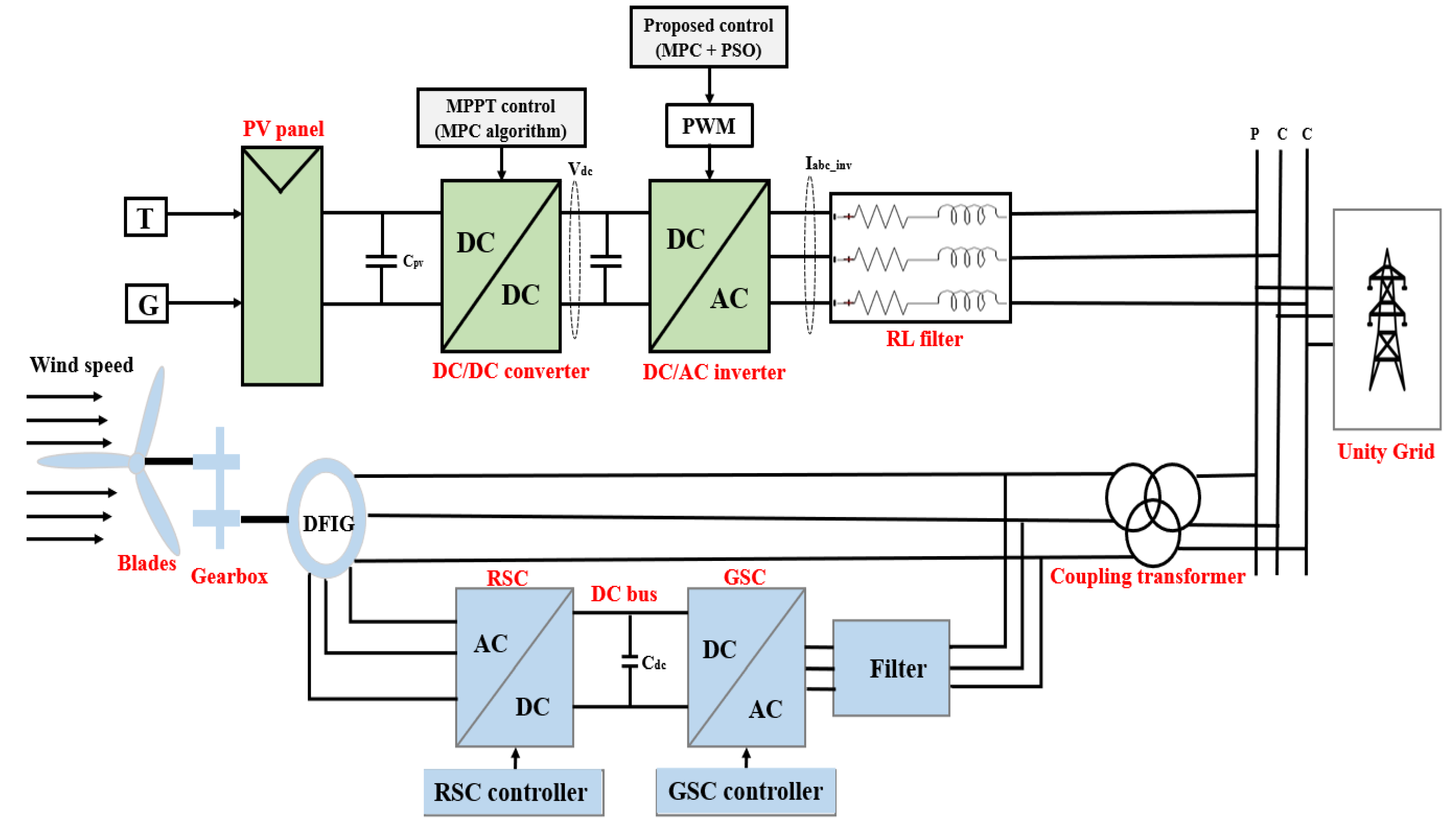
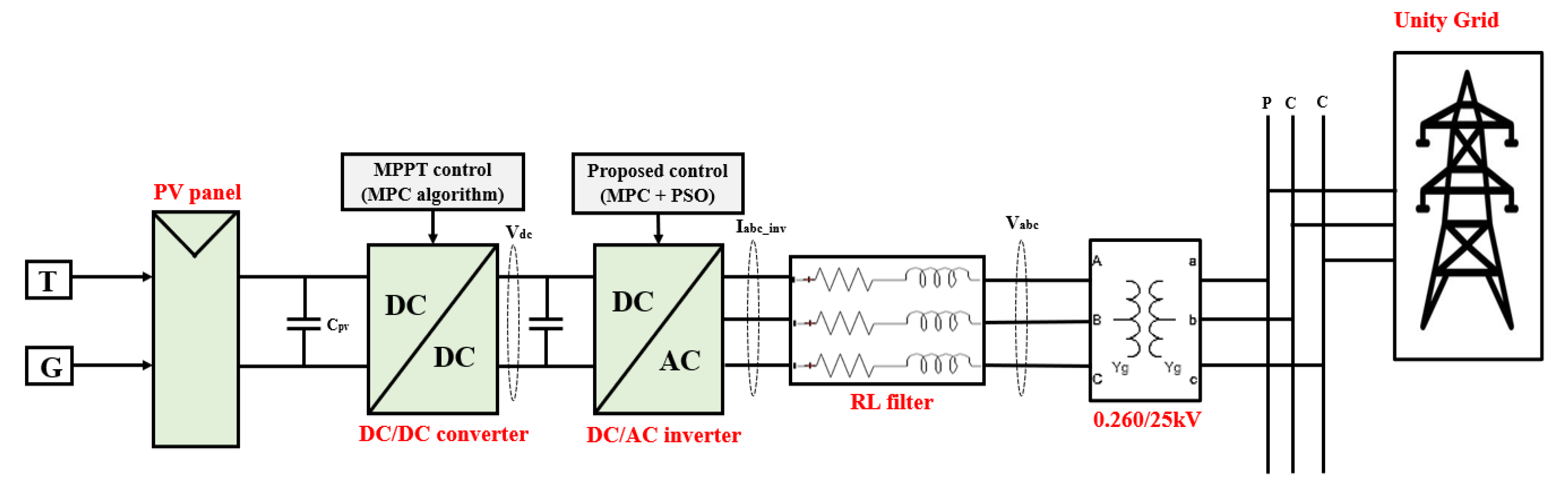
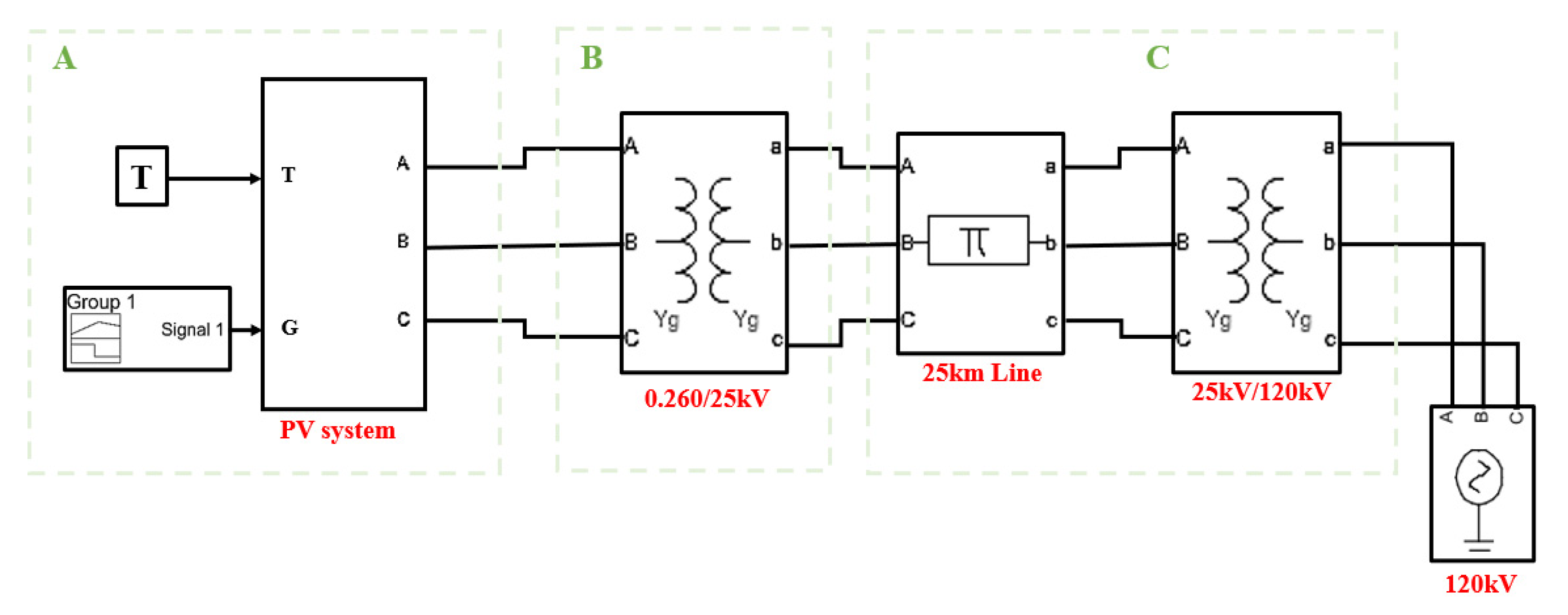
2. Configuration of Hybrid System
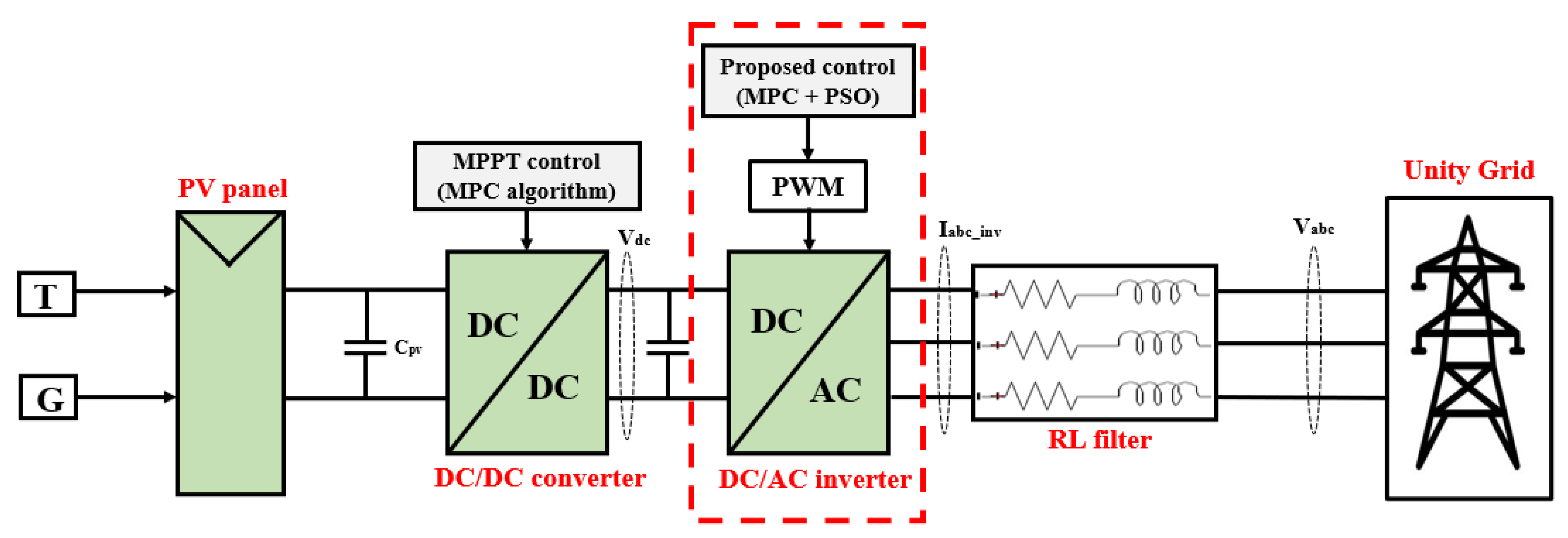
3. Description of Photovoltaic System Configuration
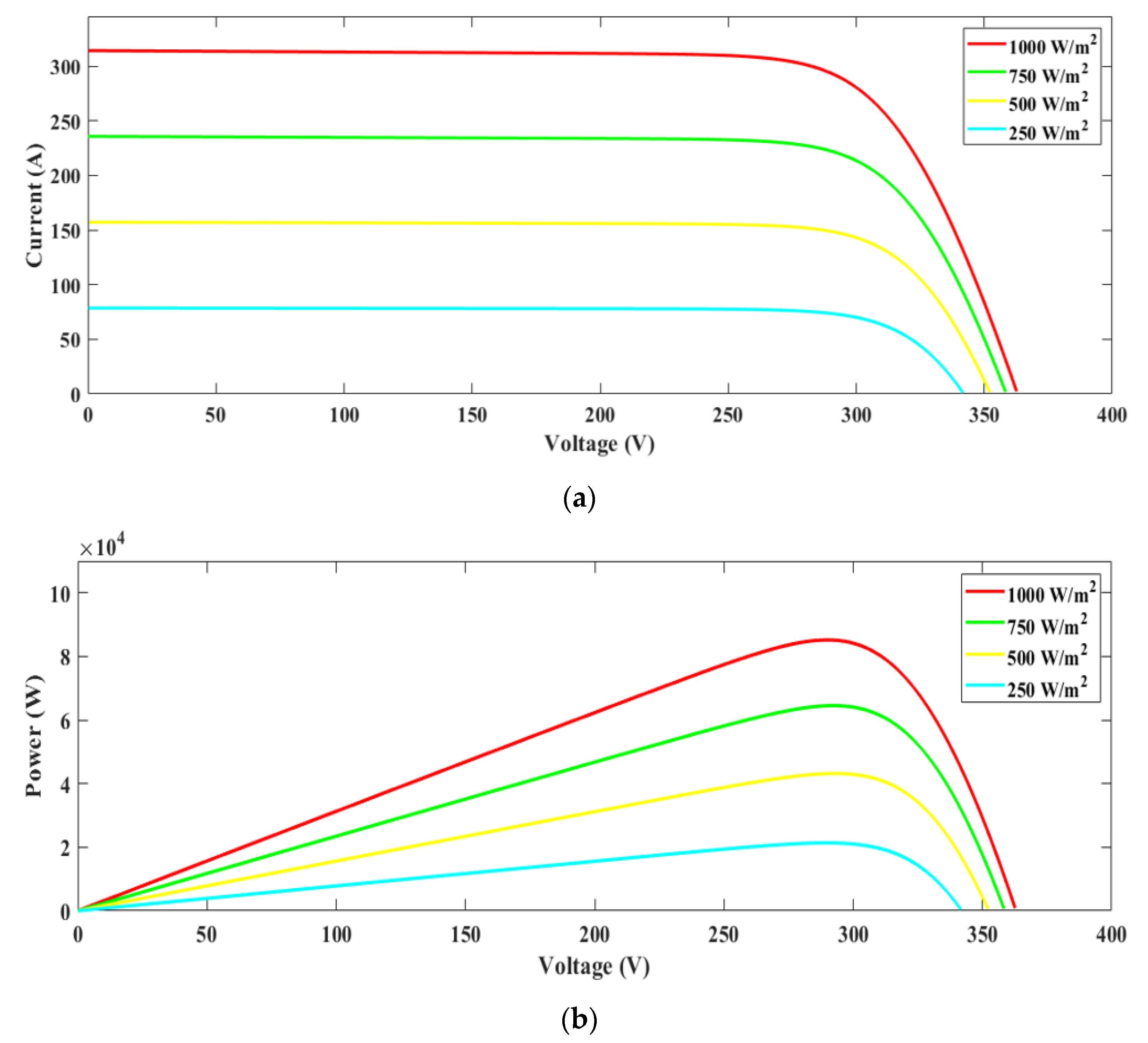
3.1. Photocell Panel
- : The current output from the PV generator.
- : The temperature-dependent saturation current of the diode.
- : The current induced by photon absorption.
- : The current flowing through the shunt resistance.
- : The benchmark short-circuit current at standard test conditions.
- : The current’s response coefficient to temperature variations.
- : The Boltzmann constant.
- : The charge of an electron.
- : The quality factor of the diode, also known as the ideality factor.
- : The thermal voltage.
- and : The number of modules connected in parallel and cells connected in series, respectively.
- : The rated saturation current at a reference temperature.
- : The bandgap energy of the semiconductor material used.
- and : The inherent series and shunt resistances within the PV module.
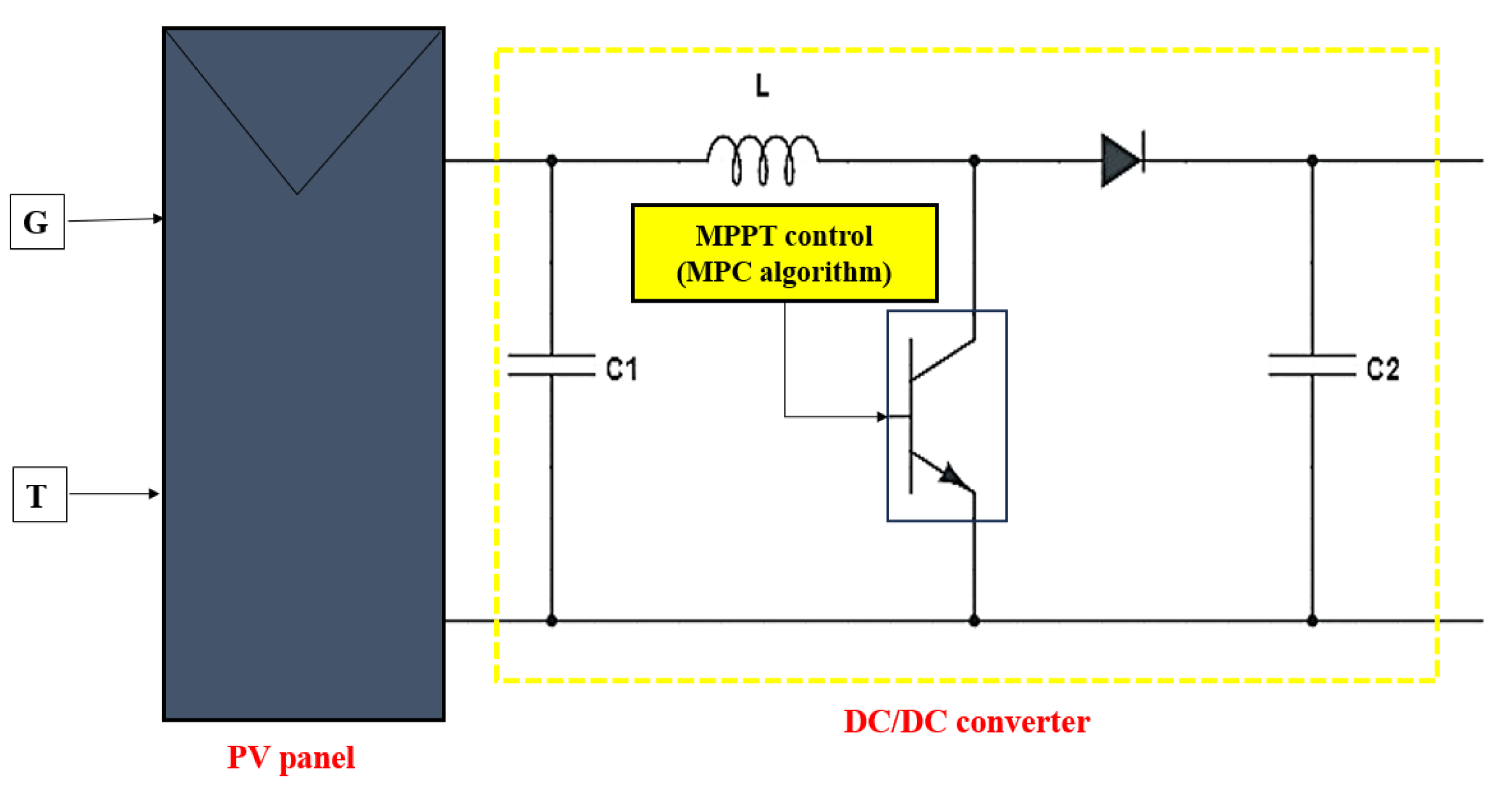
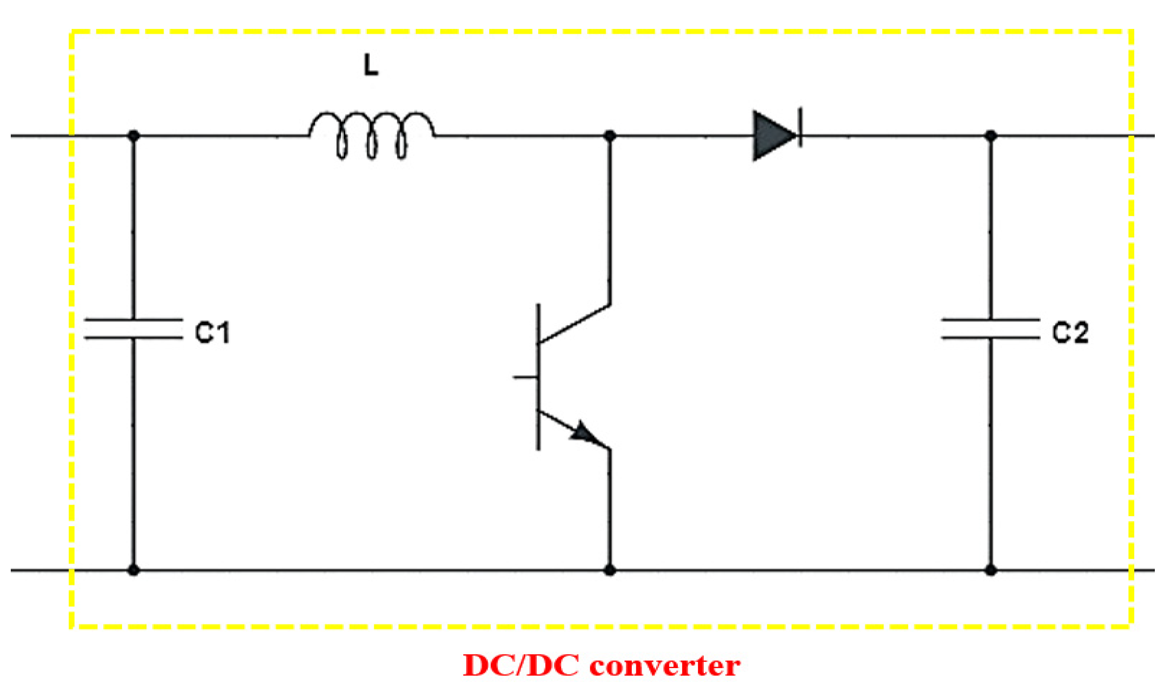
3.2. MPPT
- : Voltage generated by the photovoltaic system;
- : Current produced by the photovoltaic system;
- : Voltage across the capacitance in the boost converter, representing the output voltage target for the boost converter;
- : Capacitance within the boost converter circuit.
3.3. MPPT MPC
- : represents the parameter subject to discretization.
- : denotes the sampling period.
- : signifies the discrete time steps.
3.4. Stability of MPPT MPC “Lyapunov”
3.4.1. Selection of the Lyapunov Function
3.4.2. Affirmation of Lyapunov Function’s Positivity
3.4.3. Determination of the Lyapunov Function’s Discrete Differential
3.4.4. Criterion for the Non-Positive Differential
3.4.5. Global Stability Overview
3.4.6. Cost Function’s Role in Promoting Stability
3.5. DC/AC Inverter Control Strategy
3.6. MPC Controller for DC–AC Inverter
3.6.1. Model Predictive Control Implementation
3.6.2. MPC Optimization with PSO
3.6.3. Stability Analysis of DC–AC Inverter Control System
- Proposition of a Lyapunov Function: For the given system, we propose a Lyapunov function rooted in the stored energy within the inductances, corresponding to the sum of the squares of the currents and :
- Affirmation of Function Positivity: It is evident that is positive across all and values, as it constitutes a sum of squares of these current components.
- Calculation of the Lyapunov Function Difference: The change in the Lyapunov function, , is expressed as:
- D.
- Verification of Non-Positive Difference: The subsequent step involves demonstrating that remains non-positive for all k.
- E.
- Correlation of Cost Function to Stability: The cost function J aims to minimize the discrepancy between the predicted currents and and their reference counterparts and . Theoretically, perfect minimization at each step should steer the system towards the reference values, suggesting stability in terms of error convergence towards zero.
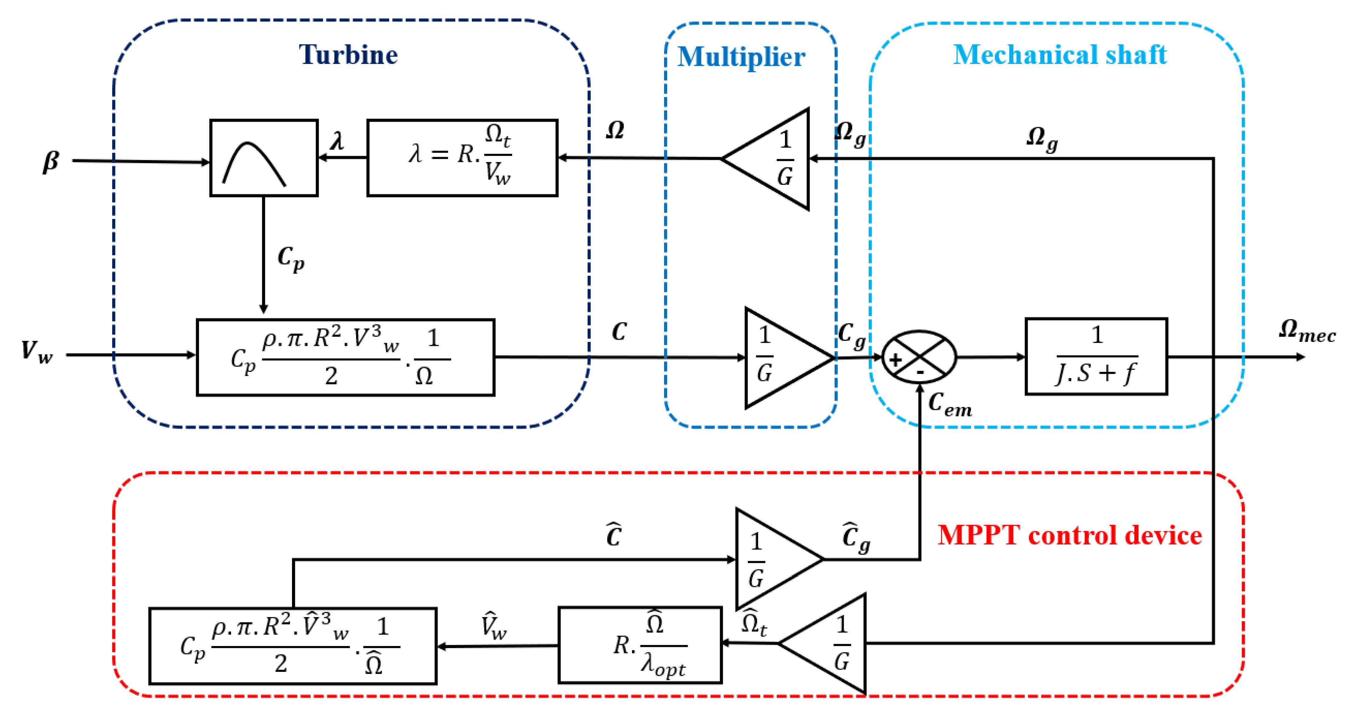
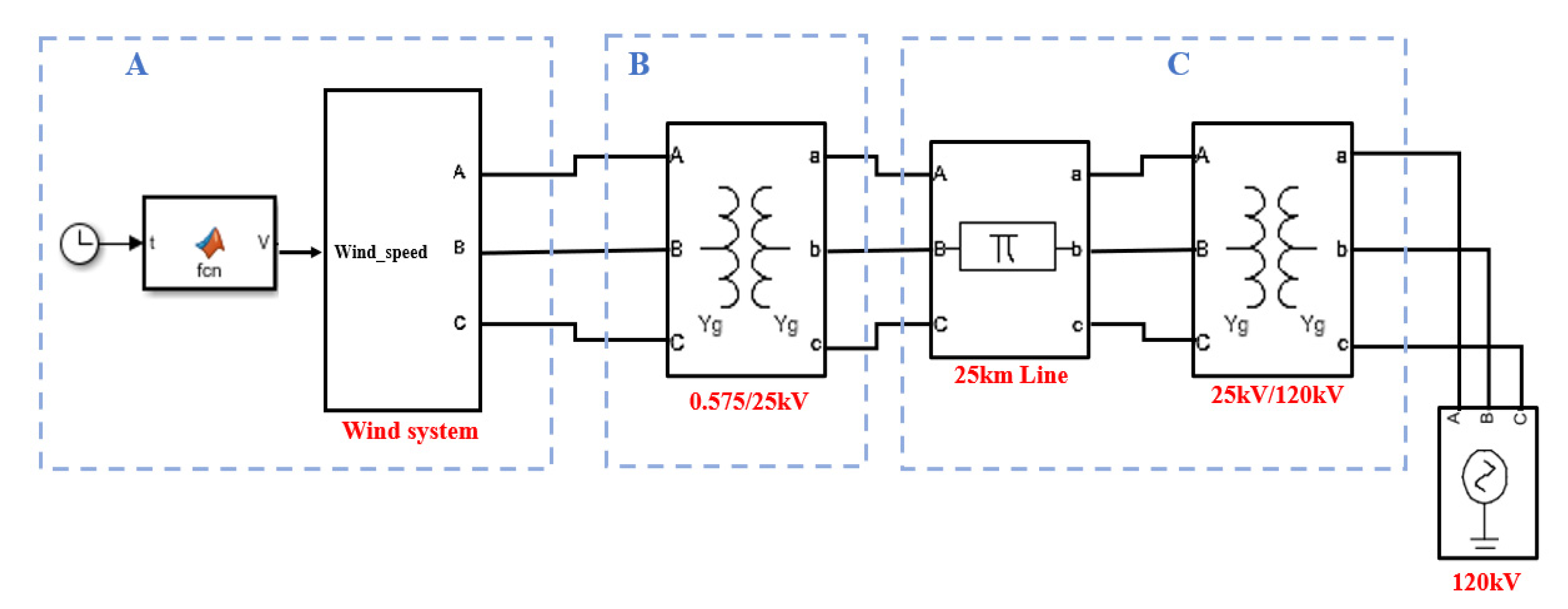
4. Description of Wind System Configuration
4.1. Overview of Wind Power
4.1.1. Wind Energy Model
4.1.2. Doubly Fed Induction Generator (DFIG) Modeling
4.1.3. Rotor-Side Converter (RSC) Control in DFIG System
4.1.4. Modeling of the Grid-Side Converter (GSC)
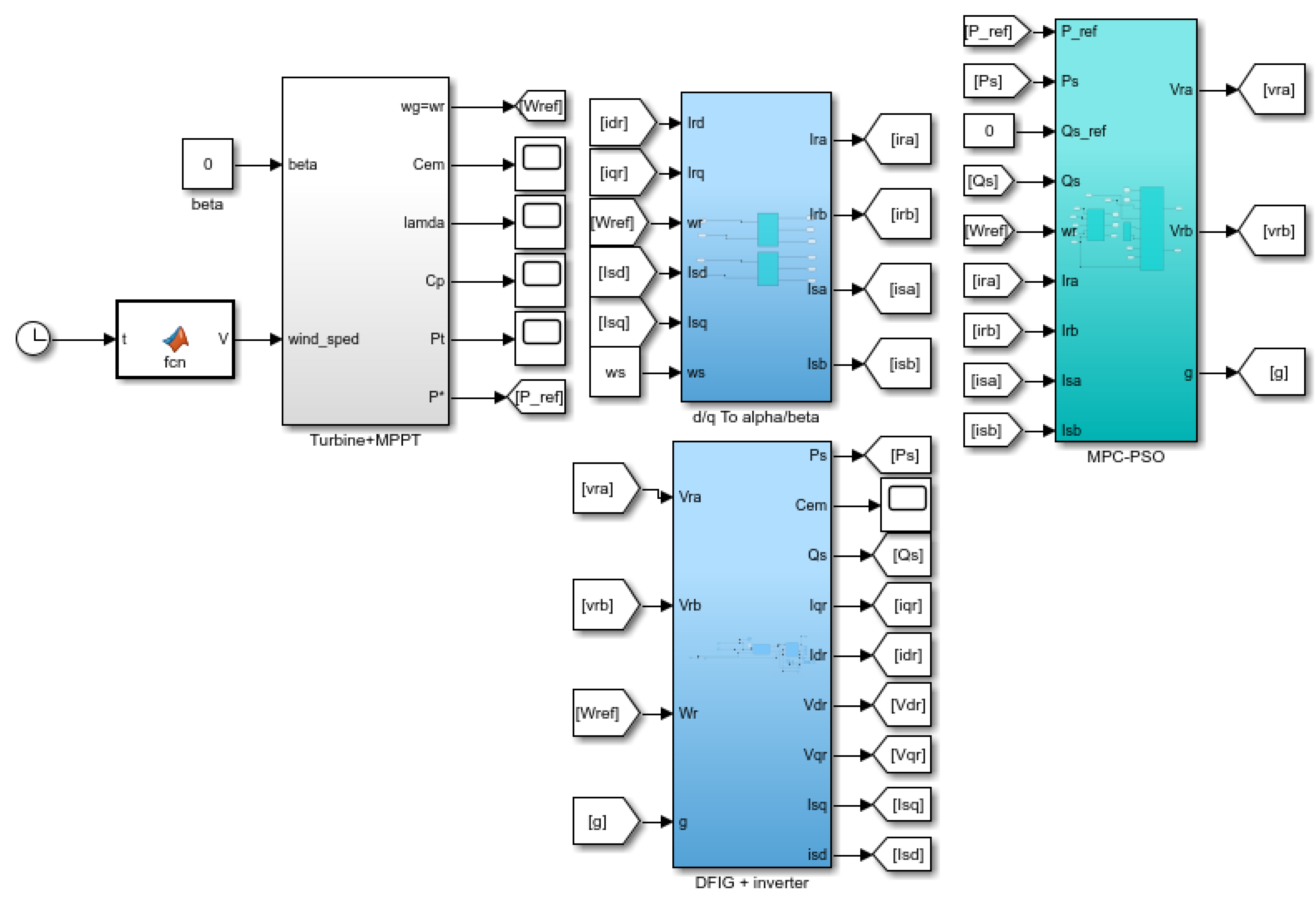
4.2. MPC Controller Optimizing by PSO
RSC Controller
- Defining Control Aspirations and Modeling: At the heart of RSC functionality within wind turbine applications lies the imperative to modulate rotor currents, and , to oversee the electromagnetic torque and manage reactive power. Such regulation is vital to synchronize rotor velocity with a pre-set reference, compensating for wind speed fluctuations.
- Strategizing MPC Coupled with PSO: The MPC establishes an optimization challenge with the goal of curtailing a cost metric emblematic of the control goals within a forecast horizon constrained by the dynamics inherent to the RSC. Concurrently, PSO is woven into the MPC structure, tasked with the identification of prime control stratagems, an endeavor facilitated by its heuristic nature to canvass the extensive parameter space.
- Lyapunov Function Proposition: Asserting stability involves positing a Lyapunov function, , indicative of the system’s energy reserves. For RSC systems, might encapsulate the electrical energy within the rotor’s inductive components and the rotor’s kinetic vigor:
- D.
- Lyapunov Function Derivative Derivation: The crux of stability validation necessitates the derivative of , , to be non-positive along system trajectories. The exercise entails computing the temporal rate of change in and integrating the RSC’s dynamical behavior:
- E.
- Implementation of MPC+PSO for Lyapunov Derivative Minimization:
- F.
- Simulation for Empirical Corroboration:
- G.
- Enhanced Stability Assurance of Grid-Side Converters via an Integrated MPC-PSO Control Paradigm
5. Simulation and Results
5.1. For PV System
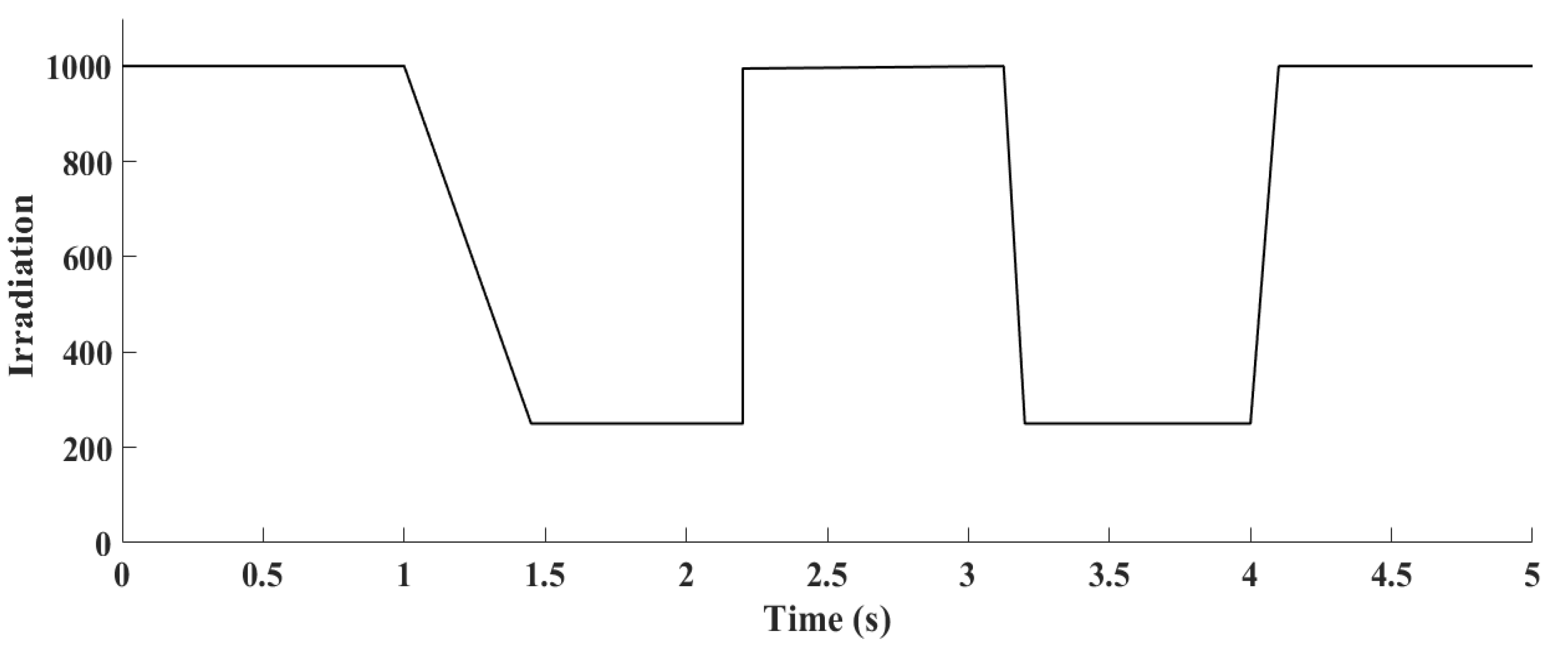
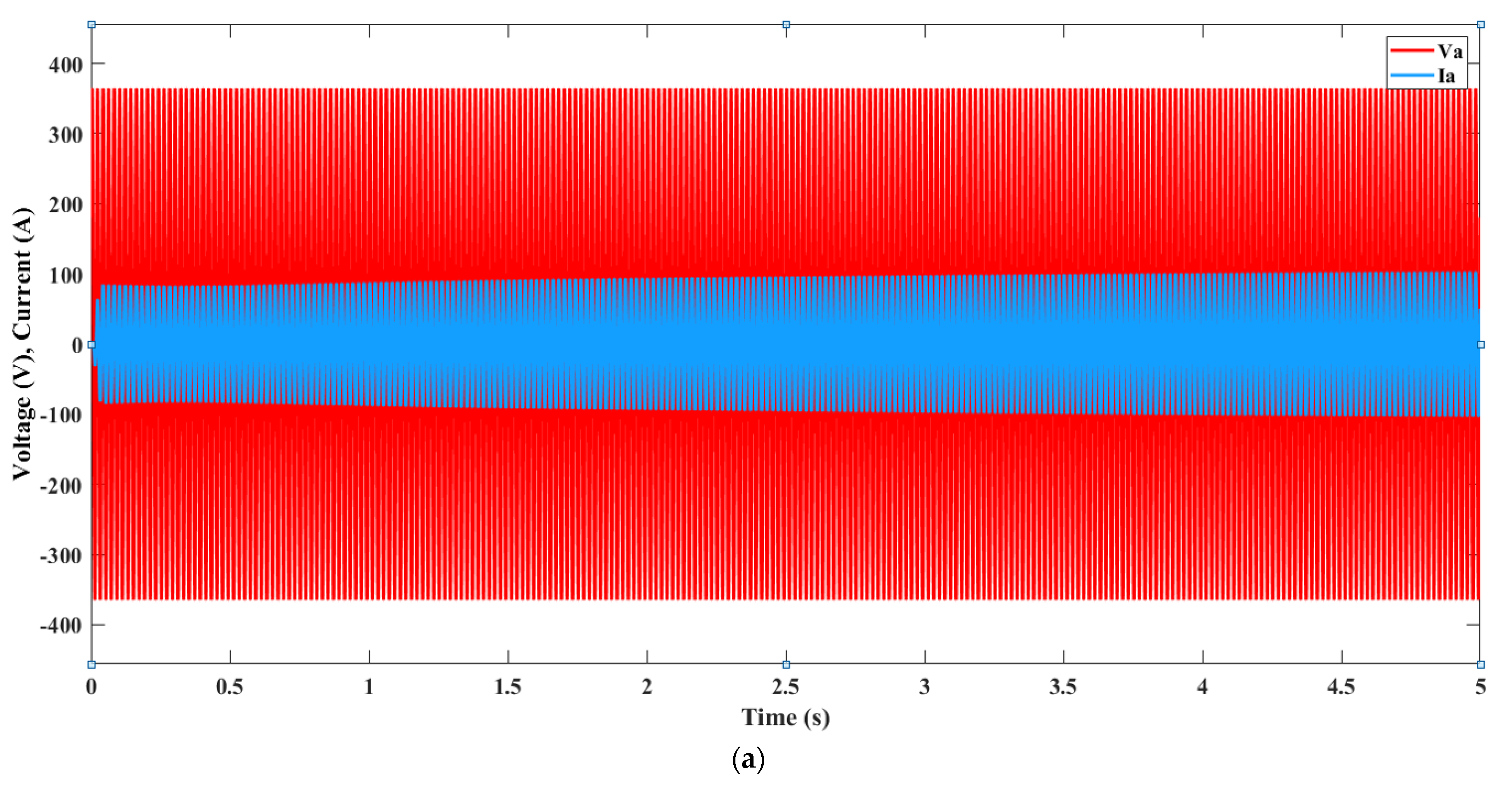
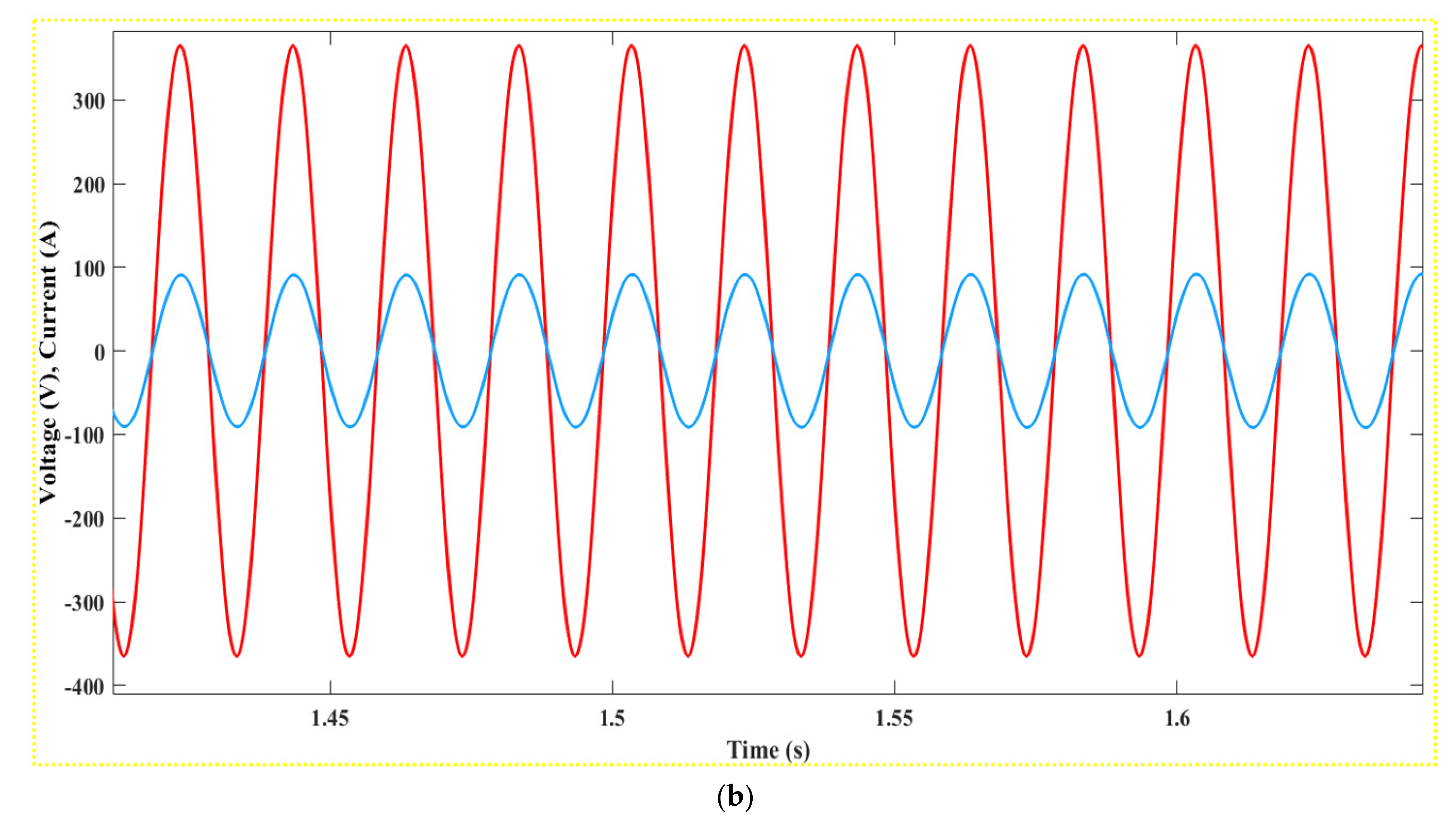
5.2. Simulation
5.3. Results
5.3.1. Part A
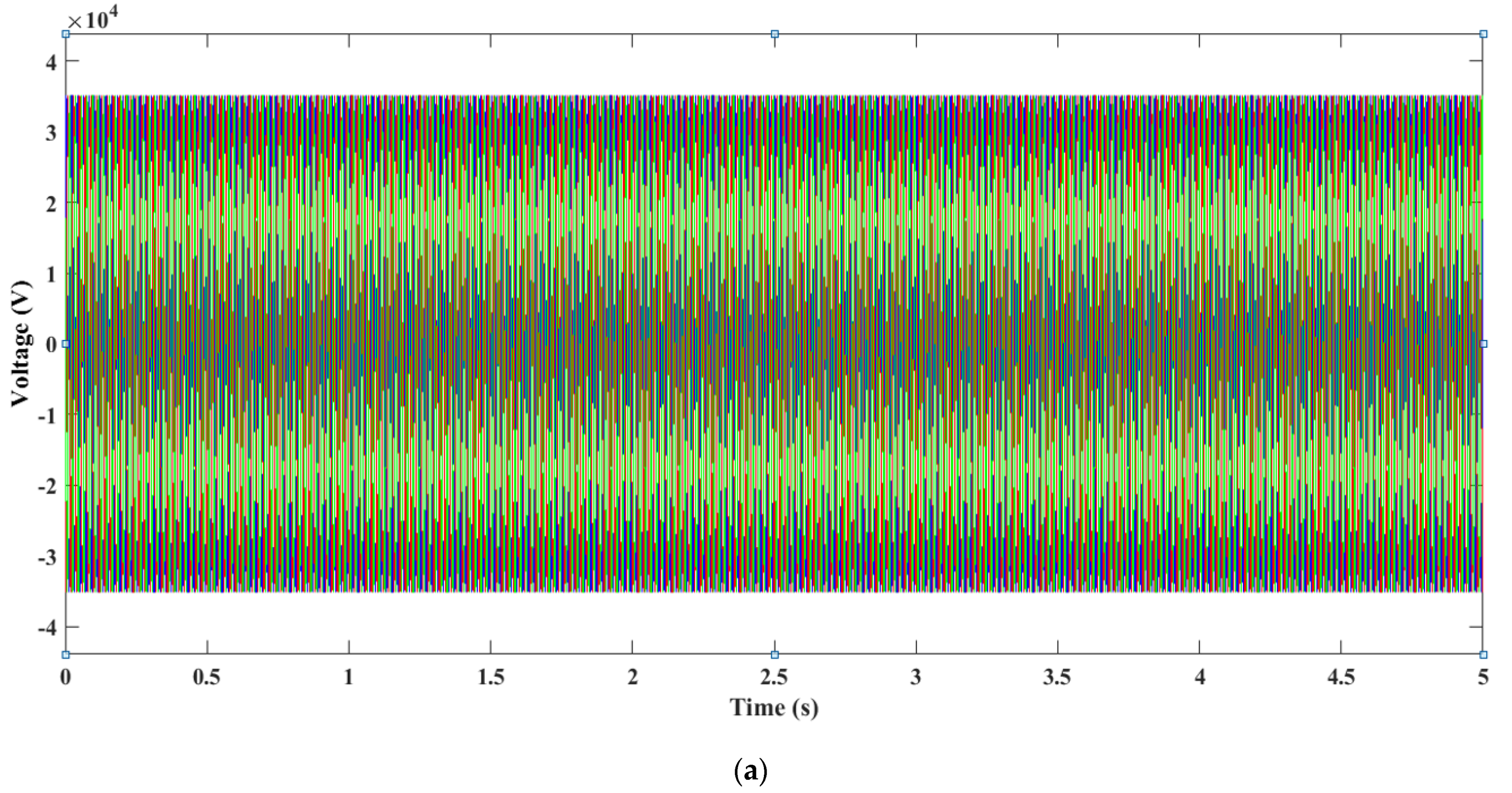
5.3.2. Part B
5.3.3. Part C
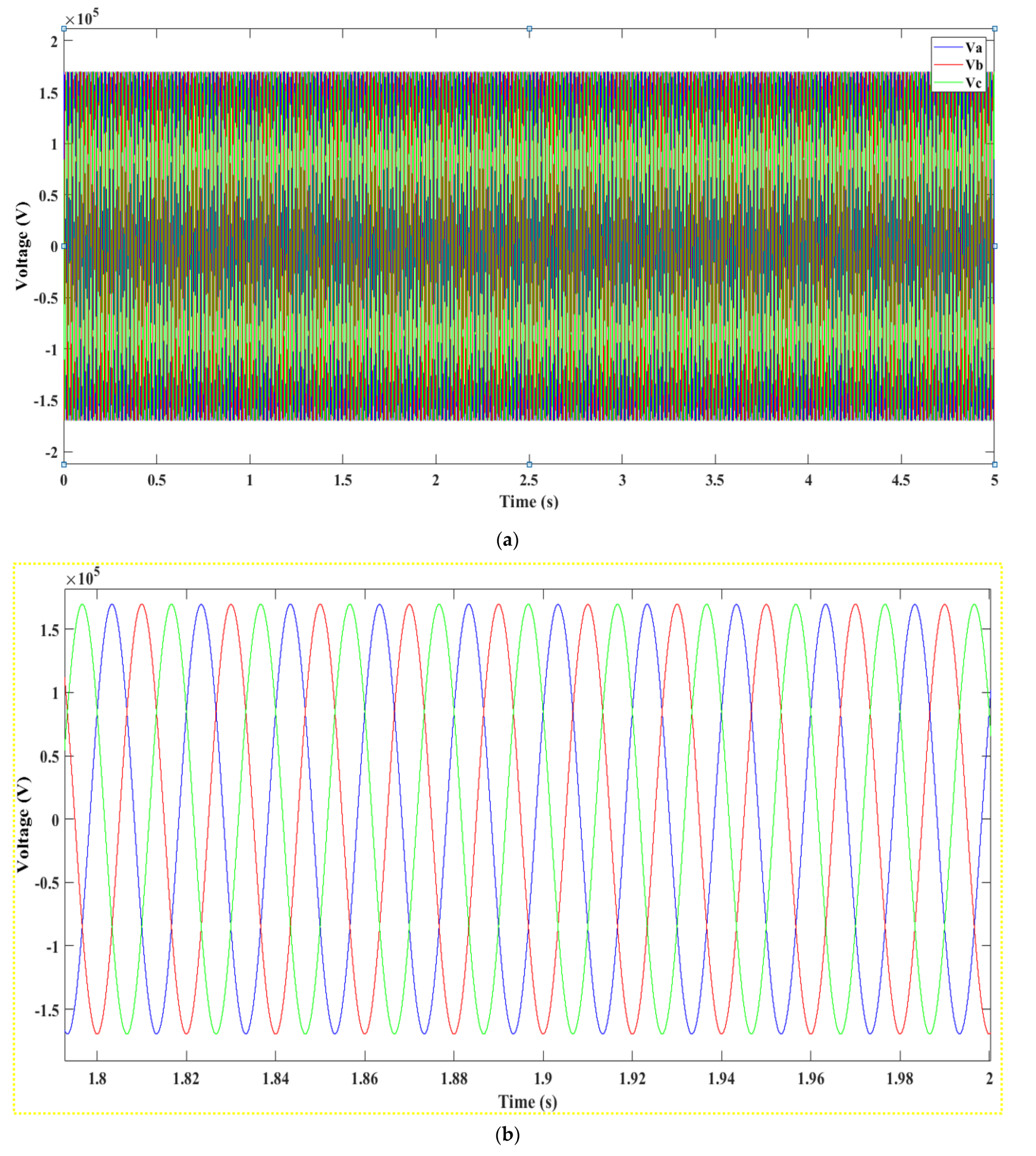
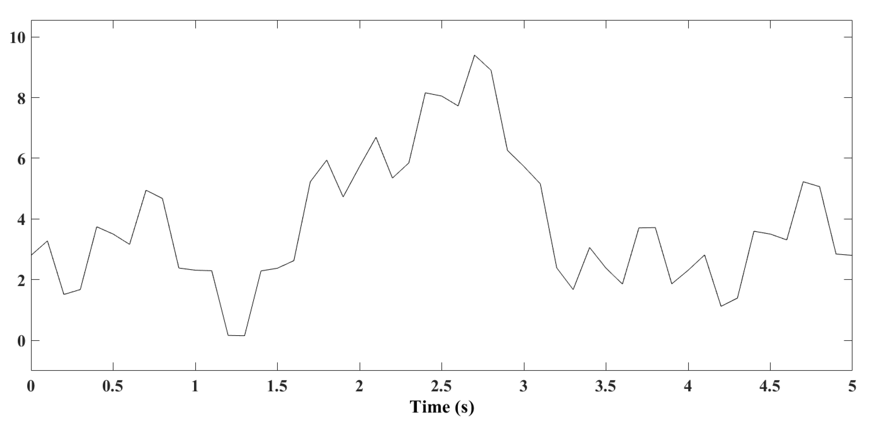
5.4. Simulation
5.5. Results
5.5.1. Part A
5.5.2. Part B
5.5.3. Part C
5.6. Hybrid System
5.6.1. Simulation
5.6.2. Results
6. Conclusions
Author Contributions
Funding
Institutional Review Board Statement
Informed Consent Statement
Data Availability Statement
Conflicts of Interest
References
- Ishaque, K.; Salam, Z. A review of maximum power point tracking techniques of PV system for uniform insolation and partial shading condition. Renew. Sustain. Energy Rev. 2013, 19, 475–488. [Google Scholar] [CrossRef]
- Tolba, M.; Rezk, H.; Diab, A.A.Z.; Al-Dhaifallah, M. A Novel Robust Methodology Based Salp Swarm Algorithm for Allocation and Capacity of Renewable Distributed Generators on Distribution Grids. Energies 2018, 11, 2556. [Google Scholar] [CrossRef]
- Tolba, M.A.; Rezk, H.; Tulsky, V.; Diab, A.A.Z.; Abdelaziz, A.Y.; Vanin, A. Impact of Optimum Allocation of Renewable Distributed Generations on Distribution Networks Based on Different Optimization Algorithms. Energies 2018, 11, 245. [Google Scholar] [CrossRef]
- Cheng, Z.; Zhou, H.; Yang, H. Research on MPPT control of PV system based on PSO algorithm. In Proceedings of the 2010 Chinese Control and Decision Conference, Xuzhou, China, 26–28 May 2010; pp. 887–892. [Google Scholar]
- Singh, G.K. Solar power generation by PV (photovoltaic) technology: A review. Energy 2013, 53, 1–13. [Google Scholar] [CrossRef]
- Baloch, M.H.; Chauhdary, S.T.; Ishak, D.; Kaloi, G.S.; Nadeem, M.H.; Wattoo, W.A.; Younas, T.; Hamid, H.T. Hybrid Energy Sources Status of Pakistan: An Optimal Technical Proposal to Solve the Power Crises Issues. Energy Strategy Rev. 2019, 24, 132–153. [Google Scholar] [CrossRef]
- Lun, S.; Du, C.; Sang, J.; Guo, T.; Wang, S.; Yang, G. An improved explicit I–V model of a solar cell based on symbolic function and manufacturer’s datasheet. Sol. Energy 2014, 110, 603–614. [Google Scholar] [CrossRef]
- Bai, J.; Liu, S.; Hao, Y.; Zhang, Z.; Jiang, M.; Zhang, Y. Development of a new compound method to extract the five parameters of PV modules. Energy Convers. Manag. 2014, 79, 294–303. [Google Scholar] [CrossRef]
- Baloch, M.; Abro, S.; Sarwar Kaloi, G.; Mirjat, N.; Tahir, S.; Nadeem, M.; Gul, M.; Memon, Z.; Kumar, M. A Research on Electricity Generation from Wind Corridors of Pakistan (Two Provinces): A Technical Proposal for Remote Zones. Sustainability 2017, 9, 1611. [Google Scholar] [CrossRef]
- Vidhya, K.; Arfan, G.; Erping, Z. Modelling and simulation of maximum power point tracking algorithms and review of MPPT techniques for PV applications. In Proceedings of the 5th International Conference on Electronic Devices, Systems and Applications (ICEDSA), Ras Al Khaimah, United Arab Emirates, 6–8 December 2016; pp. 1–4. [Google Scholar]
- Nandurkar, S.R.; Rajeev, M. Modeling simulation & design of photovoltaic array with MPPT control techniques. Int. J. Appl. Power Eng. (IJAPE) 2014, 3, 41–50. [Google Scholar]
- Babaa, S.E.; Armstrong, M.; Pickert, V. Overview of maximum power point tracking control methods for PV systems. J. Power Energy Eng. 2014, 2, 59–72. [Google Scholar] [CrossRef]
- Faranda, R.; Leva, S. Energy comparison of MPPT techniques for PV systems. WSEAS Trans. Power Syst. 2008, 3, 446–455. [Google Scholar]
- Singh, G.; Lentijo, S.; Sundaram, K. The impact of the converter on the reliability of a wind turbine generator. In Proceedings of the ASME 2019 Power Conference, Salt Lake City, UT, USA, 15–18 July 2019; V001T06A016. ASME: New York, NY, USA, 2019. [Google Scholar]
- Singh, G.; Matuonto, M.; Sundaram, K. Impact of imbalanced wind turbine generator cooling on reliability. In Proceedings of the 2019 10th International Renewable Energy Congress (IREC), Sousse, Tunisia, 26–28 March 2019; IEEE: New York, NY, USA, 2019; pp. 1–6. [Google Scholar] [CrossRef]
- Singh, G.; Saleh, A.; Amos, J.; Sundaram, K.; Kapat, J. IC6A1A6 vs. IC3A1 Squirrel Cage Induction Generator Cooling Configuration Challenges and Advantages for Wind Turbine Application. In Proceedings of the ASME 2018 Power Conference Collocated with the ASME 2018 12th International Conference on Energy Sustainability and the ASME 2018 Nuclear Forum, Lake Buena Vista, FL, USA, 24–28 June 2018; V001T06A002. ASME: New York, NY, USA, 2018. [Google Scholar]
- Orosz, T.; Rassõlkin, A.; Kallaste, A.; Arsénio, P.; Pánek, D.; Kaska, J.; Karban, P. Robust Design Optimization and Emerging Technologies for Electrical Machines: Challenges and Open Problems. Appl. Sci. 2020, 10, 6653. [Google Scholar] [CrossRef]
- Youcef, B. Contribution à L’étude et à la Commande Robuste d’un Aérogénérateur Asynchrone à Double Alimentation. Ph.D. Thesis, Université Mohamed Khider, Biskra, Algeria, 2014. [Google Scholar]
- Guda, S.R. Modeling and Power Management of a Hybrid Wind-Microturbine Power Generation. Master’s Thesis, Université de Bozeman, Bozeman, MT, USA, 2005. [Google Scholar]
- Hirose, T.; Matsuo, H. Standalone Hybrid Wind-Solar Power Generation System Applying Dump Power Control without Dump Load. IEEE Trans. Ind. Electron. 2012, 59, 988–997. [Google Scholar] [CrossRef]
- Hossain, M.K.; Ali, M. Transient stability augmentation of PV/DFIG/SG-based hybrid power system by parallel-resonance bridge fault current limiter. Electr. Power Syst. Res. 2016, 130, 89–102. [Google Scholar] [CrossRef]
- Parida, A.; Chatterjee, D. Cogeneration topology for wind energy conversion system using doubly-fed induction generator. IET Power Electron. 2016, 9, 1406–1415. [Google Scholar] [CrossRef]
- Bakir, H.; Kulaksiz, A.A. Modelling and voltage control of the solar-wind hybrid micro-grid with optimized STATCOM using GA and BFA. Eng. Sci. Technol. Int. J. 2020, 23, 576–584. [Google Scholar] [CrossRef]
- Pena, R.S.; Asher, G.M.; Clare, J.C. A Doubly Fed induction generator using back to back PWM converters supplying an isolated load from a variable speed wind turbine. Proc. Inst. Electr. Eng. Power Appl. 1996, 143, 380–387. [Google Scholar] [CrossRef]
- Rhouma, M.B.; Gastli, A.; Ben Brahim, L.; Touati, F.; Benammar, M. A simple method for extracting the parameters of the PV cell single-diode model. Renew. Energy 2017, 113, 885–894. [Google Scholar] [CrossRef]
- Azali, S.; Sheikhan, M. Intelligent control of photovoltaic system using BPSO-GSA-optimized neural network and fuzzy-based PID for maximum power point tracking. Appl. Intell. 2016, 44, 88–110. [Google Scholar] [CrossRef]
- Koad, R.; Zobaa, A.; Shahat, A. A Novel MPPT Algorithm Based on Particle Swarm Optimisation for Photovoltaic Systems. IEEE Trans. Sustain. Energy 2017, 8, 468–476. [Google Scholar] [CrossRef]
- Calasan, M.; Jovanovic, D.; Rubezic, V.; Mujovic, S.; Dukanovic, S. Estimation of Single-Diode and Two Diode Solar Cell Parameters by Using a Chaotic Optimization Approach. Energies J. 2019, 12, 4209. [Google Scholar] [CrossRef]
- Chowdhury, S.; Chowdhury, S.P.; Taylor, G.A.; Song, Y.H. Mathematical Modeling and Performance Evaluation of a Stand-Alone Polycrystalline PV Plant with MPPT Facility. In Proceedings of the IEEE Power and Energy Society General Meeting—Conversion and Delivery of Electrical Energy in the 21st Century, Pittsburg, PA, USA, 20–24 July 2008. [Google Scholar]
- Jung, J.-H.; Ahmed, S. Model Construction of Single Crystalline Photovoltaic Panels for Real-Time Simulation. In Proceedings of the IEEE Energy Conversion Congress and Expo, Atlanta, GA, USA, 12–16 September 2010. [Google Scholar]
- Nema, S.; Nema, R.K.; Agnihotri, G. Matlab/simulink based study of photovoltaic cells/modules/array and their experimental verification. Int. J. Energy Environ. 2010, 1, 487–500. [Google Scholar]
- Mohamed, S.A.; El Sattar, M.A. A comparative study of P and O and INC maximum power point tracking techniques for grid-connected PV systems. SN Appl. Sci. 2019, 1, 174. [Google Scholar] [CrossRef]
- Boubii, C.; Kafazi, I.E.; Bannari, R.; Bhiri, B.E. A comparison between MPC, Perturb and Observe, and Incremental Conductance Method. In Proceedings of the 2023 5th Global Power, Energy and Communication Conference (GPECOM), Nevsehir, Türkiye, 14–16 June 2023; pp. 198–202. [Google Scholar] [CrossRef]
- Rodriguez, J.; Cortes, P. Predictive Control of Power Converters and Electrical Drives; John Wiley & Sons: Hoboken, NJ, USA, 2012; Volume 37. [Google Scholar]
- Oskouei, A.B.; Banaei, M.R.; Sabahi, M. Hybrid PV/wind system with quinary asymmetric inverter without increasing DC-link number. Ain Shams Eng. J. 2016, 7, 579–592. [Google Scholar] [CrossRef]
- Kennedy, J.; Eberhart, R.C. Particle swarm optimization. In Proceedings of the IEEE International Conference on Neural Networks, Perth, WA, Australia, 27 November–1 December 1995; Volume 4, pp. 1942–1948. [Google Scholar]
- Errami, Y.; Obbadi, A.; Sahnoun, S. Control of PMSG wind electrical system in network context and during the MPP tracking process. Int. J. Syst. Control Commun. 2020, 11, 200–225. [Google Scholar] [CrossRef]
- Idrissi, I.; Chafouk, H.; El Bachtiri, R.; Khanfara, M. Modeling and Simulation of the Variable Speed Wind Turbine Based on a Doubly Fed Induction Generator [Internet]. Gas Turbines—Control, Diagnostics, Simulation, and Measurements [Working Title]. IntechOpen. 2019. Available online: https://www.intechopen.com/chapters/70671 (accessed on 28 December 2019).
- Boubii, C.; El Kafazi, I.; Bannari, R.; El Bhiri, B.; Mobayen, S.; Zhilenkov, A.; Bossoufi, B. Integrated Control and Optimization for Grid-Connected Photovoltaic Systems: A Model-Predictive and PSO Approach. Energies 2023, 16, 7390. [Google Scholar] [CrossRef]
- Boualouch, A.; Essadki, A.; Nasser, T.; Boukhriss, A.; Frigui, A. Power Control of DFIG in WECS Using Backstipping and Sliding Mode Controller. Int. J. Electr. Comput. Energetic Electron. Commun. Eng. 2015, 9, 612–618. [Google Scholar]
- Bakar, A.A.; Utomo, W.M.; Taufik, T.; Aizam Jumadril, S. Dc/dc boost converter with PI controller using real-time interface. ARPN J. Eng. Appl. Sci. 2015, 10, 9078–9082. [Google Scholar]
- Rodríguez-Amenedo, J.L.; Arnaltes, S.; Rodríguez, M.A. Operation and coordinated control of fixed and variable speed wind farms. Renew. Energy 2008, 33, 406–414. [Google Scholar] [CrossRef]
- Mishra, N.K.; Husain, Z. Novel Six Phase Doubly Fed Induction Generator through Modeling and Simulation-A Comparison with Conventional Doubly Fed Induction Generator. In Proceedings of the 2019 International Conference on Power Electronics, Control and Automation (ICPECA), New Delhi, India, 16–17 November 2019; pp. 1–5. [Google Scholar] [CrossRef]
- Mensou, S.; Essadki, A.; Minka, I.; Nasser, T.; Idrissi, B.B. Backstepping controller for a variable wind speed energy conversion system Based on a DFIG. In Proceedings of the 2017 International Renewable and Sustainable Energy Conference (IRSEC), Tangier, Morocco, 4–7 December 2017; Volume 12. [Google Scholar]
- Labdai, S.; Bounar, N.; Boulkroune, A.; Hemici, B.; Nezli, L. Artificial neural network-based adaptive control for a DFIG-based WECS. ISA Trans. 2022, 128 Pt B, 171–180. [Google Scholar] [CrossRef]
- Khojet El Khil, S. Vector Control of Doubly Fed Asynchronous Machine (MADA). Ph.D. Thesis, National Polytechnic Institute of Toulouse, Toulouse, France, 4 December 2006. [Google Scholar]
- EAbdou, H.; Youssef, A.-R.; Kamel, S.; Aly, M.M. Sensorless Wind Speed Control of 1.5 MW DFIG Wind Turbines for MPPT. In Proceedings of the 2018 Twentieth International Middle East Power Systems Conference (MEPCON), Cairo, Egypt, 18–20 December 2018; pp. 700–704. [Google Scholar] [CrossRef]


| Attribute | Details |
|---|---|
| Strings of series modules | 10 |
| Number of parallel strings | 40 |
| Model of Solar Module | 1Soltech 1STH-215P |
| Peak power capacity | 213.5 |
| Voltage at peak power | 29 |
| Current at peak power | 7.35 |
| Maximum circuit current | 7.84 |
| Voltage when open-circuited | 36.3 |
| Attribute | Details |
|---|---|
| Inductance | 0.002 |
| Capacitance | 0.00025 |
| Parameters | Value |
|---|---|
| 0.0137 Ω | |
| 0.021 Ω | |
| 0.0137 Ω | |
| 0.0136 Ω | |
| 0.0135 Ω | |
| 0.0017 | |
| 3 | |
| Sampling time Ts |
| Parameters | Value |
|---|---|
| 2 | |
| 0.8 | |
| d | 0.99 |
| bird_step | 20 |
| Parameters | Value |
|---|---|
| 5 | |
| 250 | |
| Varmin | −600 |
| Varmax | 600 |
Disclaimer/Publisher’s Note: The statements, opinions and data contained in all publications are solely those of the individual author(s) and contributor(s) and not of MDPI and/or the editor(s). MDPI and/or the editor(s) disclaim responsibility for any injury to people or property resulting from any ideas, methods, instructions or products referred to in the content. |
© 2024 by the authors. Licensee MDPI, Basel, Switzerland. This article is an open access article distributed under the terms and conditions of the Creative Commons Attribution (CC BY) license (https://creativecommons.org/licenses/by/4.0/).
Share and Cite
Boubii, C.; Kafazi, I.E.; Bannari, R.; El Bhiri, B.; Bossoufi, B.; Kotb, H.; AboRas, K.M.; Emara, A.; Nasiri, B. Synergizing Wind and Solar Power: An Advanced Control System for Grid Stability. Sustainability 2024, 16, 815. https://doi.org/10.3390/su16020815
Boubii C, Kafazi IE, Bannari R, El Bhiri B, Bossoufi B, Kotb H, AboRas KM, Emara A, Nasiri B. Synergizing Wind and Solar Power: An Advanced Control System for Grid Stability. Sustainability. 2024; 16(2):815. https://doi.org/10.3390/su16020815
Chicago/Turabian StyleBoubii, Chaymae, Ismail El Kafazi, Rachid Bannari, Brahim El Bhiri, Badre Bossoufi, Hossam Kotb, Kareem M. AboRas, Ahmed Emara, and Badr Nasiri. 2024. "Synergizing Wind and Solar Power: An Advanced Control System for Grid Stability" Sustainability 16, no. 2: 815. https://doi.org/10.3390/su16020815
APA StyleBoubii, C., Kafazi, I. E., Bannari, R., El Bhiri, B., Bossoufi, B., Kotb, H., AboRas, K. M., Emara, A., & Nasiri, B. (2024). Synergizing Wind and Solar Power: An Advanced Control System for Grid Stability. Sustainability, 16(2), 815. https://doi.org/10.3390/su16020815