Abstract
Coastal ecosystems are vulnerable due to watershed sediment and nutrient loads. In this study, the hydrology and water quality of two coastal watersheds, Wolf River watershed (WRW) and Jourdan River watershed (JRW), were assessed using the Soil and Water Assessment Tool (SWAT). Model performance evaluation was performed using the coefficient of determination (R2) and the Nash–Sutcliffe Efficiency (NSE). After model calibration and validation, the effectiveness of ponds, wetlands, riparian buffers, and their combination as best management practices (BMPs) were analyzed. Total suspended solids (TSS) was reduced by 31.15% in the pond scenario and 30.37% in the wetland in WRW. In addition, mineral phosphorous (MinP) was reduced by 11.84% and 9.63% in ponds and wetlands, respectively. Similarly, in JRW, TSS was reduced by 74.89% in ponds and 74.90% in wetlands. Likewise, ponds and wetlands reduced MinP by 8.05% and 13.40%, respectively. Among four riparian buffer scenarios, the 30 m buffer prompted the estimation of higher reductions such as TSS by 28.36% and MinP by 29.77% in WRW, whereas a 13.14% TSS and 22.89% MinP reduction in JRW. In addition, combined BMP, TSS was reduced by 30.37% and MinP by 52.09% in WRW, followed by a 74.92% reduction in TSS and 27.37% in MinP in JRW. All BMP implementations were effective in reducing TSS and MinP. This study suggests that ponds and wetlands were effective in reducing TSS and riparian buffers were effective in reducing MinP. These findings could be insightful in coastal watershed management.
1. Introduction
Anthropogenic activities [1,2,3] and extreme weather events [4] introduce pollution to coastal ecosystems. Due to the short sediment transport pathway and high precipitation, coastal watersheds are vulnerable to soil erosion [5] driving sediment and nutrient loads and impacting water quality and the critical coastal ecosystem. Maximum sedimentation causes turbidity [6] and habitat burial [7]. Nutrient over-enrichment causes intoxication [8], eutrophication [9], and ecological changes [10] in the coastal environment. Therefore, coastal sediment and nutrient pollutants need sustainable management globally [1]. Concerns regarding the deterioration of coastal watersheds were reported by Oelsner and Stets [11] considering the increasing trend of nutrient-loading from undeveloped watersheds in recent years (2002–2012) as compared to the past of the United States. The reductions in key agricultural non-point source (NPS) pollutants, i.e., sediment [12], nitrogen, and phosphorous [11] in estuaries benefit the coastal ecosystem. Therefore, a significant sediment and nutrient yield reduction can be achieved by implementing the best management practices (BMPs) in the coastal watershed [13,14].
The development of the Clean Water Act is the origin of BMPs, and its amendments incorporated the necessity of source and NPS pollution management with BMPs to reduce water pollution. The application of BMPs in the Chesapeake Bay, the largest estuary in the United States, was estimated to reduce nutrient loads by more than 50% [15]. BMPs’ application in the forest area at the coastal plain is higher compared to the piedmont and mountain regions of the southeastern United States [16]. In addition to the forests, the implementation of BMPs in agricultural land at the coastal plain has also shown substantial sediment and nutrient reduction [14,17]. A study to prioritize the watersheds among the United States Department of Agriculture (USDA), the Natural Resources Conservation Service (NRCS), and the Conservation Effects Assessment Project (CEAP), watersheds at the southeastern coastal plain ecoregion applied the cost-effectiveness and community-ranking method, which urged certain watersheds located in Alabama, Northern Florida, and Virginia to implement BMPs to reduce erosion in the ecological scale [18]. Furthermore, regarding the uncertainty of the design and efficiency of BMPs, Arnillas et al. [19] recommended undertaking a comprehensive examination of the BMPs’ efficiency database to address gaps in regional performance.
Well-calibrated, physical theory-based watershed models are suitable for studying hydrology and selecting BMPs in coastal areas [20]. Among various hydrological modelling tools, the robust interdisciplinary model Soil and Water Assessment Tool (SWAT) [21], which has been applied in varying topographies, is capable of studying the hydrology of coastal watersheds [22]. Similar to other popular hydrological models, such as the Agricultural Non-Point Source pollution model (ANGPS), Better Assessment Science Integrating Point and Non-point Sources (BASINS), Hydrologic Simulation Program Fortran (HSPF), SWAT is limited in analyzing the influence of tidal waves on the river system, but it is effective in simulating downstream flow [23]. The complexity in defining the boundary of the coastal watersheds, the runoff generation processes and pathways in shallow poorly drained soil, the evapotranspiration processes, and microtopography at the low-gradient forested watershed in the coastal plain is difficult to model accurately [24].
Upadhyay et al. [23] reported that only 0.46% of the total seven thousand plus peer-reviewed publications in the SWAT model have addressed coast, gulf, or bay in their respective research goals, where good to satisfactory hydrological simulation of the coastal watershed was concluded. Among them, the BMP effectiveness in the coastal watershed was reported by López-Ballesteros et al. [13], and an economic analysis of BMPs was reported by Shao et al. [25]. The effectiveness of individual and the combination of contour planting, filter strips, reforestation, fertilizer application and check dam restoration as BMPs is stated at the El Beal watershed, Spain in López-Ballesteros et al. [13]. Shao et al. [25] developed the Watershed Evaluation of BMPs (WEBs) with a farm economic model, SWAT model, and an optimization model to create BMP scenarios and simulate the economic cost and water quantity/quality advantages at the field, subbasin, and watershed scale. The aforementioned coupled model created BMPs scenarios with conservation tillage, nutrient management, cover crop, and water-sediment control basins at the Gully Creek watershed in Ontario, Canada, and suggested its efficacy in ranking the BMPs with respect to the cost-effectiveness, critical pollution source identification, and the tradeoffs between economy and water quality/quantity [25]. Moreover, field-based measures, including the restoration of wetlands and the implementation of riparian zones to create a sink for nitrogen running off to the Gulf of Mexico, are recommended [26].
Therefore, this study aims to assess the effectiveness of BMPs in reducing sediment yield and nutrient loss in the coastal watersheds of Mississippi using the SWAT model. The objectives of this study were: (i) To set-up, calibrate, and validate the SWAT model for stream flow, total suspended solids (TSS), and mineral phosphorous (MinP); and (ii) To assess the reduction in TSS and MinP due to the implementation of ponds, wetlands, riparian buffer, and their combination as BMP.
In this study, the SWAT model was used for the hydrological and water quality assessment to quantify the streamflow, sediment, and nutrient runoff from the coastal watersheds of Mississippi. Impoundments, such as ponds and wetlands, riparian buffers, and their combination, were used to evaluate the effectiveness of BMPs to reduce sediment and nutrient loss. This study highlights the capability of SWAT model to adequately simulate flow, sediment, and nutrient runoff in coastal watersheds, and the effectiveness of BMPs to improve the water quality of coastal water draining into the estuaries and bays.
2. Materials and Methods
2.1. Study Area
The Wolf River watershed (WRW) and Jourdan River watershed (JRW) are two adjacent watersheds located in the southern part of Mississippi State. The WRW spans over five counties: Hancock, Harrison, Pearl River, Stone, and Lamar, whereas the JRW spans over two counties: Hancock and Harrison. The estimated area of WRW is 801 km2 with a mixed land use of 54.88% forest-evergreen, 26.74% wetland-forested, 12.74% range-brush, and 5.64% pasture, and hence the primary land use is forest. Similarly, JRW is estimated to be 538 km2 with 37.44% forest-evergreen, 34.42% wetland-forest, 18.97% pasture, and 9.16% range-brush, and its land use is also dominated by forest. Geospatial data from the Mississippi Automated Resource Information System (MARIS) (https://maris.mississippi.edu/ (accessed on 15 August 2022) [27] were accessed to create a location map of the WRW and JRW in the state of Mississippi, as shown in Figure 1.
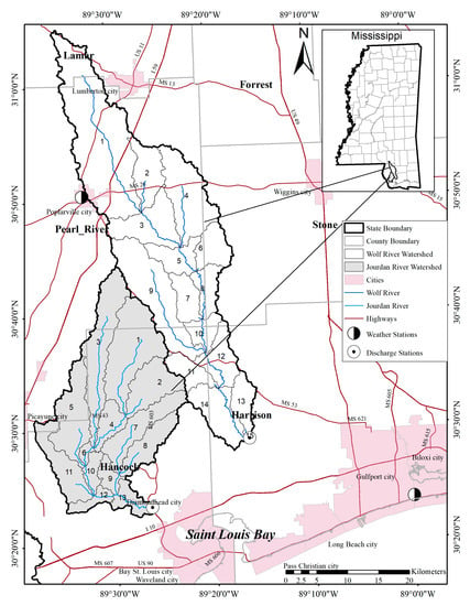
Figure 1.
Location map of Wolf River and Jourdan River watersheds in the state of Mississippi.
The Wolf River and Jourdan River are the dominant coastal streams that feed fresh water into Saint Louis Bay (SLB) from the east and west, respectively. The SLB opens into the Mississippi Sound, and as a vital part of the Mississippi Gulf Coast Region, its water quality significantly impacts the health of the Mississippi Sound [28]. Moreover, Sawant [29] emphasized the necessity for a management plan for SLB, and Spaid [30] highlighted the concern of sediment and nutrient loading in SLB to assess submarine groundwater discharge. The climate of Mississippi is hot, humid, and subtropical. At the SLB, the yearly average temperature is 19.9 °C. Typically, 98 wet days are observed throughout the year, with an average annual precipitation of 1534.2 mm. The impact of climate change on precipitation, temperature, flow, and extreme weather at WRW and JRW are discussed by Bhattarai et al. [31].
2.2. SWAT Model
The SWAT model [21], developed by the USDA Agriculture Research Service (USDA-ARS), is a comprehensive GIS-based, watershed scale interdisciplinary model used for simulating runoff, assessing hydrological impacts under the changing environment, and quantifying NPS pollution [32] in varying topographies. The SWAT model was operated on the Arc SWAT 2012 interface on ArcGIS 10.7 during this study. SWAT uses elevation data and outlet coordinates to delineate a watershed. Thus, delineated watershed is divided into smaller sub-watersheds and further into various discrete hydrological response units (HRUs) based on the unique combination of the land use, soil, and slope type of the watershed for a detailed hydrological analysis [33]. This study adopts the SWAT model because of its detailed documentation, ease of process-based understanding, comprehensive field-based modelling approach, and supplementary automatic calibration tool.
2.3. Dataset and Model Setup
The SWAT model requires a large detailed continuous dataset during model development and simulation. The United States Geological Survey (USGS) Digital Elevation Model (DEM) (30 m × 30 m resolution) data (https://apps.nationalmap.gov/ (accessed on 15 May 2022) [34] were used to delineate the watershed into different subbasins and unique hydrologic response units. The USDA National Agriculture Statistics Service (NASS) CropScape Cropland Data Layer (https://nassgeodata.gmu.edu/CropScape/ (accessed on 15 May 2022) [35], along with the SWAT-United States Soil Survey Geographic Database (SSURGO) soil data (https://swat.tamu.edu/data/ (accessed on 15 May 2022) [36] were input in the model, and the slope classes were defined. HRU thresholds were defined as 10% for each of the following: land use surface over the subbasin, soil class percentage over land use area, and slope class percentage over soil area. Thus, the HRUs were created on the basis of the unique land use, soil, and slope class of each watershed. The WRW was divided into 15 sub-watersheds and 450 HRUs, and the JRW was divided into 13 sub-watersheds and 219 HRUs. The meteorological dataset from the National Oceanic and Atmospheric Administration (NOAA) (https://www.ncdc.noaa.gov/cdo-web/ (accessed on 16 May 2022) [37] was used for local weather data collection from two nearby weather stations, the Poplarville Experimental Station, MS, US (USC00227128), and Biloxi, MS, US (USC00220792) stations for precipitation and temperature data. Weather stations are approximately at the distance of 2 km and 28 km from the WRW boundary and 12 km and 42 km from the JRW boundary, respectively.
In accordance with the literature published on improving SWAT forest simulation, adjustments were made to the land cover/plant growth database (.dat) on forest-evergreen crop type parameters. Maximum potential leaf area index (BLAI) = 3.7 [38], Optimal temperature for plant growth (T_OPT) = 24 °C (28), Minimum (base) temperature for plant growth (T_BASE) = 4 °C [39], and the Fraction of tree biomass accumulate each year that is converted to residue during dormancy (BIO_LEAF) = 0.02 [39,40] were adjusted to address the insufficient biomass and leaf area index generated by the SWAT model on forest lands [39].
Furthermore, for management operations (.mgt), the plant/beginning growing season was scheduled by heat units from the first year followed by auto-irrigation and auto-fertilization. Auto-irrigation was applied with the water-stress identifier (WSTRS_ID) = plant-water demand, auto-irrigation source code (IRR_SCA = 1) from the individual reach of the respective subbasin as with the auto-irrigation source location (IRR_NOA) being 1 through 15 for WRW, and 1 through 13 for JRW. Additionally, auto-fertilization was applied using urea as the fertilizer in the fertilizer identification number (AFERT_ID).
The models for WRW and JRW were set up and ran for 23 years (2000–2022). Along with two years as a warmup period, streamflow simulations were performed on a monthly time step for WRW and on a daily time step for JRW at the Wolf River gauge station (USGS 02481510) and the Jourdan River gauge station (USGS02481660) (https://waterdata.usgs.gov/ms/nwis/ (accessed on 18 May 2022) [41], respectively, which are located at the outlet of the delineated watersheds. Furthermore, daily calibrations and validations of the models were performed for selected water quality parameters with the data collected bimonthly at their respective gauge stations.
2.4. Model Parameterization
The variation in the sensitivity of model parameters was analyzed using an auto-calibration tool: SWAT Calibration and Uncertainty Programs (SWAT-CUP) Sequential Uncertainty Fitting Version2 (Sufi-2) [42]. The parameterization procedure illustrates the response due to different parameters in the model. Thus, different parameters were evaluated within their realistic range, and the sensitive parameters were identified using the t-test statistic and p-value in SWAT-CUP. All parameters fitted for the models of WRW and JRW are listed in Table 1 for streamflow calibration, Table 2 for TSS calibration, and Table 3 for MinP calibration.

Table 1.
Parameters used for the calibration of streamflow in Wolf River watershed (WRW) and Jourdan River watershed (JRW).

Table 2.
Parameters used for the calibration of total suspended solids (TSS) in Wolf River watershed (WRW) and Jourdan River watershed (JRW).

Table 3.
Parameters used for the calibration of mineral phosphorus (MinP) in Wolf River watershed (WRW) and Jourdan River watershed (JRW).
2.5. Best Management Practices
BMPs aids in source water protection [43], and they are implemented in coastal plains to reduce erosion [44]. Frequently, computer models are used to anticipate the effects of BMPs at the watershed scale [45]. Therefore, in this study, ponds, wetlands, riparian buffers, and their combination were implemented as structural BMPs in the WRW and JRW models, and their efficacy was evaluated.
2.5.1. Pond
Pond is water impoundment made by excavating a pit that serves as a BMP to trap sediment and retain nutrients [46]. Assuming the fraction of the subbasin area that drains into the pond (PND_FR) as 1, a single pond is placed at the outlet of each sub-watershed where the sediment and the nutrient retained were calculated. The ponds within each sub-watershed of both WRW and JRW were identified using the USDA-National Agriculture Imagery Program (NAIP) aerial imagery (1 m × 1 m resolution) data (https://naip-usdaonline.hub.arcgis.com/ (accessed on 18 January 2023) [47], and digitized to estimate the surface area of ponds when filled to the principal spillway (ha) (PND_PSA) [48]. Furthermore, considering the average depth of 3 m [48,49], the volume of water stored in ponds when filled to the principal spillway (PND_PVOL) (104 m3 H2O) was calculated. In addition, the phosphorous settling rate in the pond (PSETLP) was considered 10 m/year, and the default value of the number of days needed to reach the target storage from the current pond storage (NDTARG) was applied in the model.
2.5.2. Wetlands
Wetlands are swamp or marsh areas that are generally covered with shallow water, which is known to reduce the flow rate and serve as a sink for eroded sediment [46] and nutrients [50]. The surface area of the wetland is determined from the United States Fish and Wildlife Service (USFWS) and the National Wetland Inventory (NWI) digital data (https://www.fws.gov/program/national-wetlands-inventory (accessed on 18 June 2022) [51], and is considered to be the maximum wetland surface area (WET_MXSA). A single impoundment cumulating all the wetland areas in one subbasin is placed at the outlet of each subbasin. The average depth of the wetland was considered 0.15 m when it reached the maximum volume, and thus, the volume of water stored in wetlands when filled to maximum water level (WET_MXVOL) (104 m3 H2O) was calculated. The surface area of wetlands at normal water level (WET_NSA) (ha) was considered 20% less than WET_MXSA, and thus, with an average depth of 0.125 m, the volume of water stored in wetlands when filled to normal water level (WET_NVOL) (104 m3 H2O) was obtained. Finally, the initial volume of water in wetlands (WET_VOL) (104 m3 H2O) was considered to be 40% of the maximum volume. The values for the fraction of the subbasin area that drains into the wetland (WET_FR), the phosphorous settling rate in the wetland (PSETLW), and the NDTARG were applied equivalently to the pond modelling scenario.
2.5.3. Riparian Forest Buffer (RFB)/Streamside Management Zones (SMZ)
RFB/SMZ are the vegetative areas maintained along the stream channel to prevent and entrap sediment and nutrients from reaching the stream [52,53]. The effectiveness of the RFB/SMZ using four scenarios (15 m, 20 m, 25 m, and 30 m) of the width of the edge-of-field filter strip (FILTERW) was analyzed at forest-evergreen and wetlands-forested land use throughout the watershed to study the effectiveness of the buffer in reducing sediment and nutrient load.
2.6. Model Performance Evaluation
The simulation performance of the hydrology and water quality of the WRW and the JRW model was evaluated based on the coefficient of determination (R2) [54] (Equation (1)) and the Nash–Sutcliff Efficiency coefficient (NSE) [55] (Equation (2)). R2 is the measure of model fit that represents the linear relation between observed and simulated data ranging from 0 to 1, where results approaching 1 indicate good model performance. The NSE determines the relative magnitude of the residual variance compared to the measured data, which indicates how well the simulated output matches the observed data along a 1:1 line (regression line with a slope equal to 1). The NSE values range from −∞ to 1. The NSE value of 1 signifies a perfect fit between the simulated and observed.
where, Oi = observed value, = mean of observed values, Si = simulated value, = mean of simulated values, and N = total number of observations [54,55].
3. Results and Discussions
3.1. Streamflow Calibration and Validation
The WRW model was calibrated from January 2002 to December 2011 and validated from January 2012 to December 2022 using the fitted parameters listed in Table 1. The performance of the WRW model in simulating the monthly streamflow at the USGS02481510 gauge station is shown in Figure 2. The model resulted in R2 from 0.49 to 0.55 and NSE from 0.48 to 0.54 during calibration and validation, respectively.
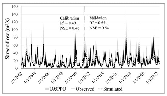
Figure 2.
Monthly streamflow calibration and validation of Wolf River watershed at USGS 02481510.
Likewise, Figure 3 shows the performance of the JRW model in simulating the daily streamflow at the USGS02481660 gauge station. The JRW model calibration was performed on a daily time scale in 2005 and the validation was performed with discontinued data from 2003 to 2004. Here, the R2 ranges from 0.34 to 0.58 during the model calibration and validation, whereas the NSE value was obtained from 0.34 to 0.56.
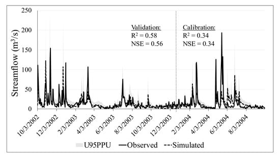
Figure 3.
Daily streamflow calibration and validation of Jourdan River watershed at USGS 02481660.
The streamflow performance of both models is consistent with other studies [56,57,58], where the limitations in the availability of continuous weather data were reported. Limited observed streamflow data and limited weather stations holding long-term continuous data within the watershed could add up for the lower streamflow performance of the models, as in compliance with Leta et al. [56], Roth et al. [57], and Zeiger et al. [58]. Therefore, gridded weather data could be a better alternative where data are limited [56,57]. Additionally, in the case of the JRW streamflow simulation, significant negative data were recorded within the limited 3 years of the discontinuous observed streamflow data available at the sole USGS gauge station. These negative data might have been recorded due to the influence of tidal events and storm surges.
3.2. TSS Calibration and Validation
Both the models were calibrated from 2/22/2021 to 10/7/2021 and validated from 10/21/2021 to 5/20/2022 on a daily time step for TSS. The parameters used to calibrate TSS on both models are listed in Table 2. For WRW, the calibration resulted in R2 = 0.59 and NSE = 0.38, whereas the validation resulted in R2 = 0.80 and NSE = 0.53. Likewise, the calibration validation of JRW resulted in R2 from 0.20 to 0.23 and NSE from 0.07 and 0.23. The trend of the WRW and JRW calibration and validation is shown in Figure 4 and Figure 5, respectively.
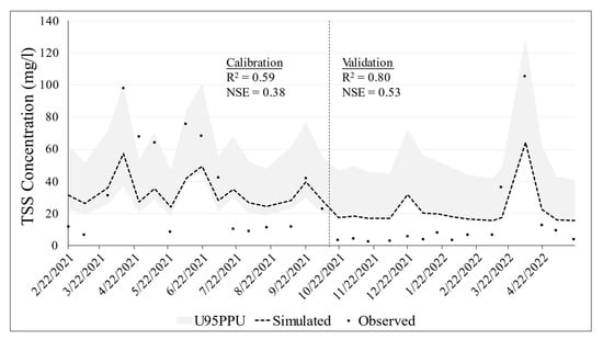
Figure 4.
Daily calibration and validation of total suspended solid (TSS) in Wolf River watershed at USGS 02481510.
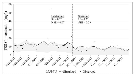
Figure 5.
Daily calibration and validation of total suspended solid (TSS) in Jourdan River watershed at USGS 02481660.
3.3. MinP Calibration and Validation
Similar to the TSS calibration validation, both the WRW and JRW models were calibrated and validated for MinP from 2/22/2021 to 10/7/2021, and 10/21/2021 to 5/20/2022, respectively, on a daily time step, and their respective fitted parameters are listed in Table 3. The calibration resulted in R2 = 0.36 and NSE = 0.26, whereas the validation resulted in R2 = 0.85 and NSE = 0.50 for WRW. Likewise, in JRW, the R2 ranges from 0.50 to 0.84, and the NSE ranges from 0.47 to 0.84. Figure 6 and Figure 7 show the trend of the MinP calibration and validation for the WRW and JRW, respectively.
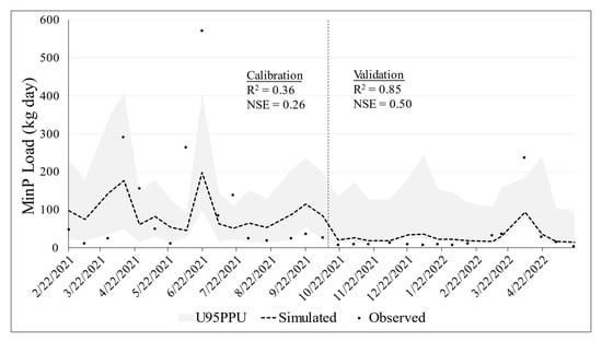
Figure 6.
Daily calibration and validation of mineral phosphorous (MinP) in Wolf River watershed USGS 02481510.
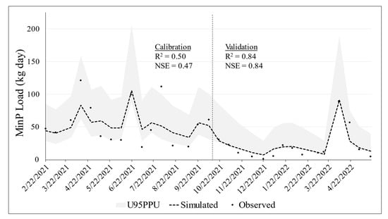
Figure 7.
Daily calibration and validation of mineral phosphorous (MinP) in Jourdan River watershed at USGS 02481660.
These results of TSS and MinP are considerably better than or similar to Addis et al. [59], Dechmi et al. [60], and Molina-Navarro et al. [61] for daily time step simulation. In Figure 4, we can observe the tendency of the SWAT model to attain the peak TSS load by overestimating other lower TSS loads as stated by Chiang et al. [62]. Extreme events, particularly flash floods, were recorded (https://www.ncdc.noaa.gov/stormevents/ (accessed on 28 June 2022) [63] in the study area on the day or within a few days prior to the data collection, which introduced peaks in both the TSS and MinP observation and simulation trend. It is also crucial to comprehend all the sediment and nutrient contribution sources throughout the watershed to obtain a better model performance [58].
3.4. Effectiveness of BMPs
Pond, wetland, RFB/SMZ, and their combination were implemented on both the WRW and JRW models to study the effectiveness of BMPs on annual average sediment and nutrient load at the coastal watershed of Mississippi. The reduction in TSS and MinP with the implementation of BMPs in outlets of WRW and JRW are shown in Figure 8 and Figure 9, respectively.
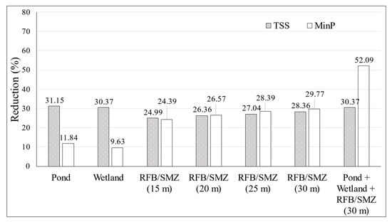
Figure 8.
Percentage reduction in total suspended solids (TSS) and mineral phosphorus (MinP) by pond, wetland, different scenarios of RFB/SMZ, and their combination in the outlet of Wolf River watershed at USGS 02481510.
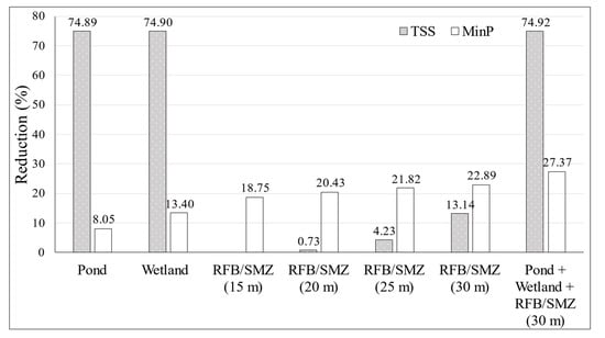
Figure 9.
Percentage reduction in total suspended solids (TSS) and mineral phosphorus (MinP) by pond, wetland, different scenarios of RFB/SMZ and their combination in the outlet of Jourdan River watershed USGS02481660.
3.4.1. Effectiveness of Pond
Ponds present in 14 subbasins of the WRW were implemented in the WRW model. The TSS load at the watershed outlet was reduced by 31.15% and MinP by 11.84%. Similarly, in the JRW, ponds present in six subbasins were implemented in the JRW model, where the TSS was reduced by 74.89% and MinP was reduced by 8.05%. Similar findings were reported in Risal and Parajuli [48] for the reduction in TSS by pond as BMP. This high reduction in TSS in JRW is comparable to Fiener et al. [64], where up to 85% reduction in sediment was attained by the pond. A comparison of sediment and nutrient reduction in Fiener et al. [64] illustrated less reduction in nutrients than sediment by pond. Alami et al.’s [65] study at the Sofichai watershed highlighted the effectiveness of detention ponds in reducing sediment and the effectiveness of filter strip in reducing MinP, whereas our findings show the effectiveness of ponds in reducing both sediment and MinP in both watersheds.
3.4.2. Effectiveness of Wetland
The implementation of inherent wetland in the WRW model demonstrated a TSS reduction of 30.37% and a MinP reduction of 9.63% at the outlet. Similarly, in the JRW model, the TSS was reduced by 74.90% and MinP was reduced by 13.04%. Sediment reduction by wetland is considerably better than Bekele et al. [66] and Leh et al. [67]. A total of 96% reduction in sediment is reported at the Beaver Dam River headwaters watershed by impoundment (pond/wetland total) in Jalowska and Yuan [68]; therefore, higher TSS reduction obtained in JRW is also justifiable. Our study demonstrates that wetland systems can reduce MinP loads in a manner similar to the pond scenario.
3.4.3. Effectiveness of RFB/SMZ
Four scenarios with different widths of RFB/SMZs were implemented on both models. In WRW, the TSS yield decreased by 24.99%, 26.36%, 27.04%, and 28.36%, whereas the MinP decreased by 24.39%, 26.57%, 28.39%, and 29.77% by the implementation of 15 m, 20 m, 25 m, and 30 m RFB/SMZ, respectively. Likewise, in JRW, no reduction in TSS was observed in the 15 m RFB/SMZ, although 0.73%, 4.23%, and 13.14% reductions were observed with 20 m, 25 m, and 30 m RFB/SMZ at the watershed outlet. In addition, 18.75%, 20.43%, 21.82%, and 22.89% reductions can be observed in the MinP yield. Hence, maximum efficiency was observed with the implementation of a 30 m RFB/SMZ in both the watershed for TSS and MinP reduction. Moreover, the application of a larger width riparian buffer filter (i.e., 35 m and 40 m) showed no further reduction in TSS and MinP load in this study. Since MinP is sorbed in sediment particles [69], we can see correspondence in the trend of TSS and MinP reduction. Saksa et al. [70] has described sediment quantification as a challenging task in low-gradient topography at the coastal plain, as in JRW; therefore, the failure of 15 m RFB/SMZ can be justified as inadequate width in low-gradient watershed with this study. This result follows the pattern of the Sirabahenda et al. [71] study regarding the sediment-trapping efficiency of riparian buffer, and is in line with Elçi [69] regarding MinP reduction.
3.4.4. Effectiveness of Pond, Wetland, and RFB/SMZ Combined
The pond, wetland, and the most efficient 30 m RFB/SMZ were combined and implemented in both watersheds. In WRW, the combination BMP decreased by 30.37% TSS and 52.09% MinP. Likewise, in JRW, it decreased by 74.92% TSS and 27.37% MinP. It is notable that combination BMPs demonstrated greater potential than individual BMPs [72,73]. Our result illustrates a similar status since combination BMPs demonstrated substantial reduction in MinP and modest improvements in TSS reduction, as compared to the reduction by individual BMP.
4. Conclusions
BMPs implementation can help to achieve the goal of reducing sediment and nutrient pollutants from coastal watersheds and prevent the degradation of the critical coastal ecosystem. This study explored the qualitative and quantitative assessment BMPs implementation of coastal watershed hydrology at the WRW and JRW, located in southern Mississippi. The effectiveness of ponds, wetlands, RFB/SMZ, and their combination as BMPs in managing the water resource and maintaining the water quality at coastal watershed draining into the coastal waters was also demonstrated. All selected structural BMP implementation was effective in reducing TSS and MinP in both watersheds. Amongst the individual BMP applications, maximum TSS reduction was obtained by the implementation of impoundment, and maximum MinP reduction was obtained by the 30 m RFB/SMZ. Although all applied BMPs performed well in both coastal watersheds, the 15 m RFB/SMZ did not show the difference in TSS yield at the JRW outlet. Since JRW is a low-gradient watershed, a 15 m RFB/SMZ alone might not be the best conservation practice. Nonetheless, an increment in the width of the RFB/SMZ to 20 m, 25 m, and 30 m has demonstrated its efficiency in reducing the sediment and nutrient load. In addition, the implementation of the combined BMP also demonstrated effectiveness in TSS and MinP reduction. Overall, from the BMP effectiveness analysis, we can conclude that impoundments are effective in entrapping TSS and riparian buffers are effective in reducing MinP.
This study reports a SWAT model application in the hydrological and water quality assessment of WRW and JRW, representing the coastal watersheds of Mississippi. The amount of sediment yield and nutrient loads from these coastal watersheds flowing into SLB could be insightful in assessing the extent of water pollution entering the bay ecosystem. This research can aid in developing watershed-scale management plans for coastal plain watersheds based on the suitable BMPs analyzed in this study. In addition, watershed hydrology, sediment, and nutrient-loading results from the SWAT model can benefit the development of the hydrodynamic models concerning river–bay–estuary linkage to understand the inter-relation of marine and freshwater hydrodynamics, and could also benefit the submarine groundwater discharge studies to comprehend the aquatic ecosystem issue.
Author Contributions
S.B.: Methodology, model development, data analysis, and writing—original draft. P.B.P.: methodology, supervision, funding acquisition, and writing—reviewing and editing. All authors have read and agreed to the published version of the manuscript.
Funding
This project was paid for in part with federal funding from the U.S. Department of the Treasury, the Mississippi Department of Environmental Quality, and the Mississippi-Based RESTORE Act Center of Excellence under the Resources and Ecosystems Sustainability, Tourist Opportunities, and Revived Economies of the Gulf Coast States Act of 2012 (RESTORE Act). The statements, findings, conclusions, and recommendations are those of the authors and do not necessarily reflect the views of the Department of the Treasury, the Mississippi Department of Environmental Quality, or the Mississippi-Based RESTORE Act Center of Excellence.
Institutional Review Board Statement
Not applicable.
Informed Consent Statement
Not applicable.
Data Availability Statement
Not applicable.
Acknowledgments
We would like to acknowledge the partial support of the Bagley College of Engineering, Mississippi Agricultural and Forestry Experiment Services (MAFES), and the College of Agriculture and Life Sciences at Mississippi State University, the United States Geological Survey (USGS), and all our collaborators in this study.
Conflicts of Interest
The authors declare that they do not have any possible financial interests or personal relationships that could have influenced the work. No conflict of interest is declared by the authors.
References
- Lu, Y.; Yuan, J.; Lu, X.; Su, C.; Zhang, Y.; Wang, C.; Cao, X.; Li, Q.; Su, J.; Ittekkot, V.; et al. Major Threats of Pollution and Climate Change to Global Coastal Ecosystems and Enhanced Management for Sustainability. Environ. Pollut. 2018, 239, 670–680. [Google Scholar] [CrossRef] [PubMed]
- Bini, M.; Rossi, V. Climate Change and Anthropogenic Impact on Coastal Environments. Water 2021, 13, 1182. [Google Scholar] [CrossRef]
- Lu, Y.; Wang, P.; Wang, C.; Zhang, M.; Cao, X.; Chen, C.; Wang, C.; Xiu, C.; Du, D.; Cui, H.; et al. Multiple Pollutants Stress the Coastal Ecosystem with Climate and Anthropogenic Drivers. J. Hazard. Mater. 2022, 424, 127570. [Google Scholar] [CrossRef]
- Babcock, R.C.; Bustamante, R.H.; Fulton, E.A.; Fulton, D.J.; Haywood, M.D.E.; Hobday, A.J.; Kenyon, R.; Matear, R.J.; Plagányi, E.E.; Richardson, A.J.; et al. Severe Continental-Scale Impacts of Climate Change Are Happening Now: Extreme Climate Events Impact Marine Habitat Forming Communities along 45% of Australia’s Coast. Front. Mar. Sci. 2019, 6, 411. [Google Scholar] [CrossRef]
- Browning, T.N.; Sawyer, D.E. Vulnerability to Watershed Erosion and Coastal Deposition in the Tropics. Sci. Rep. 2021, 11, 1–11. [Google Scholar] [CrossRef]
- Kitchener, B.G.; Wainwright, J.; Parsons, A.J. A Review of the Principles of Turbidity Measurement. Prog. Phys. Geogr. 2017, 41, 620–642. [Google Scholar] [CrossRef]
- Cunning, R.; Silverstein, R.N.; Barnes, B.B.; Baker, A.C. Extensive Coral Mortality and Critical Habitat Loss Following Dredging and Their Association with Remotely-Sensed Sediment Plumes. Mar. Pollut. Bull. 2019, 145, 185–199. [Google Scholar] [CrossRef]
- Paerl, H.W.; Otten, T.G. Harmful Cyanobacterial Blooms: Causes, Consequences, and Controls. Microb. Ecol. 2013, 65, 995–1010. [Google Scholar] [CrossRef]
- Breitburg, D.L.; Craig, J.K.; Fulford, R.S.; Rose, K.A.; Boynton, W.R.; Brady, D.C.; Ciotti, B.J.; Diaz, R.J.; Friedland, K.D.; Hagy, J.D.; et al. Nutrient Enrichment and Fisheries Exploitation: Interactive Effects on Estuarine Living Resources and Their Management. Hydrobiologia 2009, 629, 31–47. [Google Scholar] [CrossRef]
- Shaver, E.C.; Shantz, A.A.; McMinds, R.; Burkepile, D.E.; Vega Thurber, R.L.; Silliman, B.R. Effects of Predation and Nutrient Enrichment on the Success and Microbiome of a Foundational Coral. Ecology 2017, 98, 830–839. [Google Scholar] [CrossRef] [PubMed]
- Oelsner, G.P.; Stets, E.G. Recent Trends in Nutrient and Sediment Loading to Coastal Areas of the Conterminous U.S.: Insights and Global Context. Sci. Total Environ. 2019, 654, 1225–1240. [Google Scholar] [CrossRef] [PubMed]
- Thrush, S.F.; Hewitt, J.E.; Cummings, V.J.; Ellis, J.I.; Hatton, C.; Lohrer, A.; Norkko, A. Muddy Waters: Elevating Sediment Input to Coastal and Estuarine Habitats. Front. Ecol. Environ. 2004, 2, 299–306. [Google Scholar] [CrossRef]
- López-Ballesteros, A.; Senent-Aparicio, J.; Srinivasan, R.; Pérez-Sánchez, J. Assessing the Impact of Best Management Practices in a Highly Anthropogenic and Ungauged Watershed Using the SWAT Model: A Case Study in the El Beal Watershed (Southeast Spain). Agronomy 2019, 9, 576. [Google Scholar] [CrossRef]
- Fox, R.J.; Fisher, T.R.; Gustafson, A.B.; Koontz, E.L.; Lepori-Bui, M.; Kvalnes, K.L.; Bunnell-Young, D.E.; Gardner, J.R.; Lewis, J.; Winsten, J.R.; et al. An Evaluation of the Chesapeake Bay Management Strategy to Improve Water Quality in Small Agricultural Watersheds. J. Environ. Manag. 2021, 299, 113478. [Google Scholar] [CrossRef]
- Simpson, T.W.; Weammert, S.E. Revising BMP Efficiencies for the Chesapeake Bay Watershed: Challenges and Lessons Learned. In Proceedings of the American Society of Agricultural and Biological Engineers—Conference on 21st Century Watershed Technology: Improving Water Quality and Environment 2008, Concepcion, Chile, 29 March–3 April 2008. [Google Scholar]
- Hawks, B.S.; Aust, W.M.; Bolding, M.C.; Barrett, S.M.; Schilling, E.B. Audit Procedures and Implementation Rates for Forest Water Quality Best Management Practices in the 13 Southeastern States. J. Soil Water Conserv. 2022, 77, 501–515. [Google Scholar] [CrossRef]
- Sith, R.; Watanabe, A.; Nakamura, T.; Yamamoto, T.; Nadaoka, K. Assessment of Water Quality and Evaluation of Best Management Practices in a Small Agricultural Watershed Adjacent to Coral Reef Area in Japan. Agric. Water Manag. 2019, 213, 659–673. [Google Scholar] [CrossRef]
- Jang, T.; Vellidis, G.; Kurkalova, L.A.; Boll, J.; Hyman, J.B. Prioritizing Watersheds for Conservation Actions in the Southeastern Coastal Plain Ecoregion. Environ. Manag. 2015, 55, 657–670. [Google Scholar] [CrossRef]
- Arnillas, C.A.; Yang, C.; Zamaria, S.A.; Neumann, A.; Javed, A.; Shimoda, Y.; Feisthauer, N.; Crolla, A.; Dong, F.; Blukacz-Richards, A.; et al. Integrating Watershed and Ecosystem Service Models to Assess Best Management Practice Efficiency: Guidelines for Lake Erie Managers and Watershed Modellers. Environ. Rev. 2021, 29, 31–63. [Google Scholar] [CrossRef]
- Fares, A.; El-Kadi, E.-K. Coastal Watershed Management; WIT Press: Billerica, MA, USA, 1848; ISBN 9781845640910. [Google Scholar]
- Arnold, J.G.; Srinivasan, R.; Muttiah, R.S.; Williams, J.R. Large Area Hydrologic Modeling and Assessment Part I: Model Development 1. J. Am. Water Resour. Assoc. 1998, 34, 73–89. [Google Scholar] [CrossRef]
- Wu, K.; Xu, Y.J. Evaluation of the Applicability of the SWAT Model for Coastal Watersheds in Southeastern Louisiana1. JAWRA J. Am. Water Resour. Assoc. 2006, 42, 1247–1260. [Google Scholar] [CrossRef]
- Upadhyay, P.; Linhoss, A.; Kelble, C.; Ashby, S.; Murphy, N.; Parajuli, P.B. Applications of the SWAT Model for Coastal Watersheds: Review and Recommendations. J. ASABE 2022, 65, 453–469. [Google Scholar] [CrossRef]
- Amatya, D.M.; Jha, M.K. Evaluating the SWAT Model for a Low-Gradient Forested Watershed in Coastal South Carolina. Trans. ASABE 2011, 54, 2151–2163. [Google Scholar] [CrossRef]
- Shao, H.; Yang, W.; Lindsay, J.; Liu, Y.; Yu, Z.; Oginskyy, A. An Open Source GIS-Based Decision Support System for Watershed Evaluation of Best Management Practices. JAWRA J. Am. Water Resour. Assoc. 2017, 53, 521–531. [Google Scholar] [CrossRef]
- Mitsch, W.J.; Day, J.W.; Gilliam, J.W.; Groffman, P.M.; Hey, D.L.; Randall, G.W.; Wang, N. Reducing Nitrogen Loading to the Gulf of Mexico from the Mississippi River Basin: Strategies to Counter a Persistent Ecological Problem. Bioscience 2001, 51, 373–388. [Google Scholar] [CrossRef]
- MARIS. Available online: https://maris.mississippi.edu/ (accessed on 15 August 2022).
- Liu, Z.; Kingery, W.L.; Huddleston, D.H.; Hossain, F.; Hashim, N.B.; Kieffer, J.M. Assessment of Water Quality Conditions in the St. Louis Bay Watershed. J. Environ. Sci. Heal. Part A 2008, 43, 468–477. [Google Scholar] [CrossRef] [PubMed]
- Sawant, P.A. Factors Influencing the Environmental Quality of the Bay of Saint Louis, Mississippi and Implications for Evolving Coastal Management Policies. Ph.D. Thesis, The University of Southern Mississippi, Hattiesburg, MS, USA, 2009. [Google Scholar]
- Spaid, H. Contribution of Submarine Groundwater Discharge to Select Biogeochemical Fluxes in St. Louis Bay, Mississippi. Master’s Thesis, The University of Southern Mississippi, Hattiesburg, MS, USA, 2020. [Google Scholar]
- Bhattarai, S.; Parajuli, P.B.; To, F. Comparison of Flood Frequency at Different Climatic Scenarios in Forested Coastal Watersheds. Climate 2023, 11, 41. [Google Scholar] [CrossRef]
- Wang, Y.; Jiang, R.; Xie, J.; Zhao, Y.; Yan, D.; Yang, S. Soil and Water Assessment Tool (SWAT) Model: A Systemic Review. J. Coast. Res. 2019, 93, 22–30. [Google Scholar] [CrossRef]
- Gassman, P.W.; Reyes, M.R.; Green, C.H.; Arnold, J.G.; Gassman, P.W. The Soil and Water Assessment Tool: Historical Development, Applications, and Future Research Directions. Trans. ASABE 2007, 50, 1211–1250. [Google Scholar] [CrossRef]
- USGS The National Map-Advanced Viewer. Available online: https://apps.nationalmap.gov/ (accessed on 15 May 2022).
- CropScape—NASS CDL Program. Available online: https://nassgeodata.gmu.edu/CropScape/ (accessed on 15 May 2022).
- Global Data|SWAT|Soil & Water Assessment Tool. Available online: https://swat.tamu.edu/data/ (accessed on 15 May 2022).
- NOAA Climate Data Online (CDO)-National Climatic Data Center (NCDC). Available online: https://www.ncdc.noaa.gov/cdo-web/ (accessed on 16 May 2022).
- Zhang, H.; Wang, B.; Li Liu, D.; Zhang, M.; Leslie, L.M.; Yu, Q. Using an Improved SWAT Model to Simulate Hydrological Responses to Land Use Change: A Case Study of a Catchment in Tropical Australia. J. Hydrol. 2020, 585, 124822. [Google Scholar] [CrossRef]
- Haas, H.; Reaver, N.G.; Karki, R.; Kalin, L.; Srivastava, P.; Kaplan, D.A.; Gonzalez-Benecke, C. Improving the Representation of Forests in Hydrological Models. Sci. Total Environ. 2022, 812, 151425. [Google Scholar] [CrossRef]
- Poorter, H.; Niklas, K.J.; Reich, P.B.; Oleksyn, J.; Poot, P.; Mommer, L. Biomass Allocation to Leaves, Stems and Roots: Meta-Analyses of Interspecific Variation and Environmental Control. New Phytol. 2012, 193, 30–50. [Google Scholar] [CrossRef] [PubMed]
- USGS Water Data for Mississippi. Available online: https://waterdata.usgs.gov/ms/nwis/ (accessed on 18 May 2022).
- Abbaspour, K.C. SWAT-Cup 2012. SWAT Calibration and Uncertainty Program—A User Manual; Eawag Swiss Federal Institute of Aquatic Science and Technology: Dübendorf, Switzerland, 2013. [Google Scholar]
- Abell, R.; Vigerstol, K.; Higgins, J.; Kang, S.; Karres, N.; Lehner, B.; Sridhar, A.; Chapin, E. Freshwater Biodiversity Conservation through Source Water Protection: Quantifying the Potential and Addressing the Challenges. Aquat. Conserv. Mar. Freshw. Ecosyst. 2019, 29, 1022–1038. [Google Scholar] [CrossRef]
- Hawks, B.S.; Aust, W.M.; Bolding, M.C.; Barrett, S.M.; Schilling, E.; Fielding, J.A. Linkages between Forestry Best Management Practices and Erosion in the Southeastern US. J. Environ. Manag. 2022, 305, 114411. [Google Scholar] [CrossRef] [PubMed]
- Liu, Y.; Engel, B.A.; Flanagan, D.C.; Gitau, M.W.; McMillan, S.K.; Chaubey, I. A Review on Effectiveness of Best Management Practices in Improving Hydrology and Water Quality: Needs and Opportunities. Sci. Total Environ. 2017, 601–602, 580–593. [Google Scholar] [CrossRef]
- NRCS. Conservation Practice Standard Pond (Code 378); NRCS, USA, 2022. Available online: https://www.nrcs.usda.gov/sites/default/files/2022-09/Pond_378_NHCP_CPS_2022.pdf (accessed on 20 May 2022).
- National Agriculture Imagery Program—NAIP Hub Site. Available online: https://naip-usdaonline.hub.arcgis.com/ (accessed on 18 January 2023).
- Risal, A.; Parajuli, P.B. Evaluation of the Impact of Best Management Practices on Streamflow, Sediment and Nutrient Yield at Field and Watershed Scales. Water Resour. Manag. 2022, 36, 1093–1105. [Google Scholar] [CrossRef]
- NRCS. Irrigation Guide; NRCS: Stanton, NE, USA, 1997. Available online: https://directives.sc.egov.usda.gov/OpenNonWebContent.aspx?content=17837.wba (accessed on 20 May 2022).
- Chang, H.; Makido, Y.; Foster, E. Effects of Land Use Change, Wetland Fragmentation, and Best Management Practices on Total Suspended Solids Concentrations in an Urbanizing Oregon Watershed, USA. J. Environ. Manag. 2021, 282, 111962. [Google Scholar] [CrossRef]
- National Wetlands Inventory|U.S. Fish & Wildlife Service. Available online: https://www.fws.gov/program/national-wetlands-inventory (accessed on 18 June 2022).
- Li, H. Integrating Forests into Water Quality Trading by Identifying Runoff and Sediment Yield Reduction Effect Using Swat Modeling in East Texas. Ph.D. Thesis, Stephen F. Austin State University, Austin, TX, USA, 2015. [Google Scholar]
- Mississippi Forestry Commission. Best Management Practices for Forestry in Mississippi; Mississippi Forestry Commission: Jackson, MS, USA, 2008. [Google Scholar]
- Krause, P.; Boyle, D.P.; Bäse, F. Comparison of Different Efficiency Criteria for Hydrological Model Assessment. Adv. Geosci. 2005, 5, 89–97. [Google Scholar] [CrossRef]
- Nash, J.E.; Sutcliffe, J.V. River Flow Forecasting through Conceptual Models Part I—A Discussion of Principles. J. Hydrol. 1970, 10, 282–290. [Google Scholar] [CrossRef]
- Leta, O.T.; El-Kadi, A.I.; Dulai, H.; Ghazal, K.A. Assessment of SWAT Model Performance in Simulating Daily Streamflow under Rainfall Data Scarcity in Pacific Island Watersheds. Water 2018, 10, 1533. [Google Scholar] [CrossRef]
- Roth, V.; Lemann, T. Comparing CFSR and Conventional Weather Data for Discharge and Soil Loss Modelling with SWAT in Small Catchments in the Ethiopian Highlands. Hydrol. Earth Syst. Sci. 2016, 20, 921–934. [Google Scholar] [CrossRef]
- Zeiger, S.J.; Owen, M.R.; Pavlowsky, R.T. Simulating Nonpoint Source Pollutant Loading in a Karst Basin: A SWAT Modeling Application. Sci. Total Environ. 2021, 785, 147295. [Google Scholar] [CrossRef]
- Addis, H.K.; Strohmeier, S.; Ziadat, F.; Melaku, N.D.; Klik, A. Modeling Streamflow and Sediment Using SWAT in Ethiopian Highlands. Int. J. Agric. Biol. Eng. 2016, 9, 51–66. [Google Scholar] [CrossRef]
- Dechmi, F.; Burguete, J.; Skhiri, A. SWAT Application in Intensive Irrigation Systems: Model Modification, Calibration and Validation. J. Hydrol. 2012, 470–471, 227–238. [Google Scholar] [CrossRef]
- Molina-Navarro, E.; Andersen, H.E.; Nielsen, A.; Thodsen, H.; Trolle, D. The Impact of the Objective Function in Multi-Site and Multi-Variable Calibration of the SWAT Model. Environ. Model. Softw. 2017, 93, 255–267. [Google Scholar] [CrossRef]
- Chiang, L.C.; Liao, C.J.; Lu, C.M.; Wang, Y.C. Applicability of Modified SWAT Model (SWAT-Twn) on Simulation of Watershed Sediment Yields under Different Land Use/Cover Scenarios in Taiwan. Environ. Monit. Assess. 2021, 193, 1–23. [Google Scholar] [CrossRef]
- Storm Events Database | National Centers for Environmental Information. Available online: https://www.ncdc.noaa.gov/stormevents/ (accessed on 28 June 2022).
- Fiener, P.; Auerswald, K.; Weigand, S. Managing Erosion and Water Quality in Agricultural Watersheds by Small Detention Ponds. Agric. Ecosyst. Environ. 2005, 110, 132–142. [Google Scholar] [CrossRef]
- Alami, M.T.; Abbasi, H.; Niksokhan, M.H.; Zarghami, M. Charged System Search for Optimum Design of Cost-Effective Structural Best Management Practices for Improving Water Quality. Int. J. Optim. Civ. Eng. 2018, 8, 295–309. [Google Scholar]
- Bekele, E.G.; Demissie, M.; Lian, Y. Optimizing the Placement of Best Management Practices (BMPs) in Agriculturally-Dominated Watersheds in Illinois. World Environ. Water Resour. Congr. 2011 Bear. Knowl. Sustain. 2011, 2890–2900. [Google Scholar] [CrossRef]
- Leh, M.D.; Sharpley, A.N.; Singh, G.; Matlock, M.D. Assessing the Impact of the MRBI Program in a Data Limited Arkansas Watershed Using the SWAT Model. Agric. Water Manag. 2018, 202, 202–219. [Google Scholar] [CrossRef]
- Jalowska, A.M.; Yuan, Y. Evaluation of SWAT Impoundment Modeling Methods in Water and Sediment Simulations. JAWRA J. Am. Water Resour. Assoc. 2019, 55, 209–227. [Google Scholar] [CrossRef] [PubMed]
- Elçi, A. Evaluation of Nutrient Retention in Vegetated Filter Strips Using the SWAT Model. Water Sci. Technol. 2017, 76, 2742–2752. [Google Scholar] [CrossRef] [PubMed]
- Saksa, P.; Xu, Y.J.; Stich, R. Hydrologic Influence on Sediment Transport of Low-Gradient, Forested Headwater Streams in Central Louisiana. In Proceedings of the 15th Biennial Southern Silvicultural Research Conference, Asheville, NC, USA; 2010; pp. 551–558. Available online: https://www.srs.fs.usda.gov/pubs/gtr/gtr_srs175/gtr_srs175_551.pdf (accessed on 20 May 2022).
- Sirabahenda, Z.; St-Hilaire, A.; Courtenay, S.C.; Van Den Heuvel, M.R. Assessment of the Effective Width of Riparian Buffer Strips to Reduce Suspended Sediment in an Agricultural Landscape Using ANFIS and SWAT Models. CATENA 2020, 195, 104762. [Google Scholar] [CrossRef]
- Venishetty, V.; Parajuli, P.B. Assessment of BMPs by Estimating Hydrologic and Water Quality Outputs Using SWAT in Yazoo River Watershed. Agriculture 2022, 12, 477. [Google Scholar] [CrossRef]
- Nepal, D.; Parajuli, P.B. Assessment of Best Management Practices on Hydrology and Sediment Yield at Watershed Scale in Mississippi Using SWAT. Agriculture 2022, 12, 518. [Google Scholar] [CrossRef]
Disclaimer/Publisher’s Note: The statements, opinions and data contained in all publications are solely those of the individual author(s) and contributor(s) and not of MDPI and/or the editor(s). MDPI and/or the editor(s) disclaim responsibility for any injury to people or property resulting from any ideas, methods, instructions or products referred to in the content. |
© 2023 by the authors. Licensee MDPI, Basel, Switzerland. This article is an open access article distributed under the terms and conditions of the Creative Commons Attribution (CC BY) license (https://creativecommons.org/licenses/by/4.0/).