Prediction of 1,4-Dioxane Migration in Groundwater and Evaluation of Remediation Measures in an Illegal Dumping Site Using a 2D-Numerical Model

Abstract

Illegal dumping sites are usually characterized by complex contamination situations due to the presence of multiple contamination sources. To improve the efficiency of illegal waste dumping site remediation, this study developed a numerical model considering the effects of groundwater levels and hydraulic gradient changes on remediation operations. Using this model, the most likely sources of contamination for 1,4-dioxane at an illegal waste site in Iwate Prefecture, Japan, were successfully identified (including location, amount, and time of occurrence) by reproducing historical monitoring data (from 2010 to 2022) through history matching, and future contaminant migration in groundwater was predicted. In addition, based on quantitative evaluations of the remediation measures, we found that some remediation measures, such as impermeable wall construction, while having some effects on the control of contamination spreading, may accelerate the migration of contaminants off-site due to the change of hydraulic gradient. Therefore, remediation procedures should be more carefully considered for illegal dumping sites based on an understanding of the distribution of contamination sources and hydraulic gradient evolutions.

1. Introduction

Increasing urbanization has generated various environmental issues, among which illegal dumping is an increasingly serious and costly problem with negative effects on the livability and sustainability of our communities. The problem of illegal dumping is global and particularly acute in developing countries [1,2,3,4,5]. Illegal dumping can pollute groundwater and rivers, damage soil quality, affect air quality, and negatively impact wildlife [6].

Illegal dumping sites usually contain multiple but unknown contamination sources, including the location, size, period of contamination, and contaminant composition of the sources. Moreover, the subsurface geology conditions in illegal dumping sites are also relatively complex compared to legal dumping sites [7,8], which makes the spreading behaviors of contaminants in groundwater complex. Many efforts have been made to predict the spread of contaminants in groundwater in illegal dumpsites, for example, by monitoring dumpsites or scavenger accumulations on land and by aerial photography [9,10,11]. However, due to the complexity of illegal dumping sites, monitoring techniques alone cannot evaluate the spatial spread of contamination or predict contamination in the future. At the same time, numerical analysis, in combination with simulation, is a potentially effective method for contamination behavior interpretation and prediction.

A series of remediation measures are being taken to prevent the spreading of contaminants outside from illegal dumping sites, including impermeable wall construction and groundwater pumping, chemical oxidation techniques, activated carbon techniques, and bioremediation [12,13]. However, without a sufficient understanding of contaminant-spreading behaviors, the effectiveness of such costly remediation measures has been questioned [14,15]. For instance, the pumping process has been reported to significantly affect hydraulic gradient distribution and promote the spreading of contaminants [16], which potentially promotes contaminant flow to a greater extent. In order to better plan remediation measures, it is very important to develop an efficient modeling procedure for contamination prediction.

Over the past few decades, numerical modeling has become increasingly important in the prediction of groundwater flow and contaminant transport [17,18,19]. It has been reported that modeling based on piezometric pressure head and concentration monitoring results is a possible way to identify the source of contamination and the distribution of hydraulic conductivity [20,21]. Hem et al. [17] proposed a numerical modeling process for 1,4-dioxane distribution prediction with the verification of groundwater flow in an illegal waste dumping site. They suggested that the use of numerical modeling is more precise for contaminant prediction than conventional approaches that use monitoring. However, the main limitation of the previous modeling process is the use of constant source conditions, which cannot reflect the real situation [17] in which the behavior of contamination spreading will be changed with source conditions and remediation measures being taken. In addition, the geological conditions in illegal dumpsites are usually not homogeneous and result in different hydraulic gradients at different locations, which should also be taken into account in modeling. In order to develop an effective modeling procedure for the prediction of contaminant dispersion, several non-stationary sources of contamination under the dynamic conditions of the hydraulic gradient caused by remediation activities in illegal landfills should first be specified.

The illegal dumping site used for study in this paper is located between the Iwate and Aomori prefectures in Japan, which has been reported to have severe contamination by VOCs and chlorinated solvents [22] since 1999 when illegal dumping was discovered. Particularly, higher concentrations of 1,4-dioxane than Japan’s environmental standards (0.05 mg/L) have been detected in groundwater over a wide range at this site in 2010. The significant spreading of 1,4-dioxane is related to its characteristics of high solubility, low adsorption on soil particles, and strong resistance to spontaneous biodegradation [22,23]. To date, several remediation activities, such as construction of impermeable walls and groundwater pumping, have been conducted at this site for 1,4-dioxane removal, and changes in 1,4-dioxane concentration have also been monitored for a long period. Due to the above reasons, 1,4-dioxane was targeted as the representative contaminant in this study, and based on the monitoring and remediation results of 1,4-dioxane, a new numerical modeling process was developed for this illegal dumping site, and the effect of remediation measures was also quantitatively evaluated.

The aim of this work is to develop an effective numerical model to predict future contamination in groundwater and to validate the effectiveness of remediation measures (e.g., instructing impermeable walls and pumping) based on the identification of multiple sources of contamination and under the conditions of changes in groundwater flow caused by remediation measures. In this study, the most likely contamination sources of the representative contaminants, 1,4-dioxane, including the location, amount, and discharge period, will be identified using this model by reproducing the historical spatial-temporal distribution of 1,4-dioxane in the site through historical matching. With the help of this model and based on the reproduced contamination situation, more efficient remediation measures could be designed.

2. Numerical Model for the Transport Phenomena of 1,4-Dioxane in the Aquifer

2.1. Overview of 1,4-Dioxane Contamination in the Illegal Dumping Site and Remediation History

The illegal dumping site in this study is located on a gently undulating plateau about 450 m above sea level between the Aomori prefecture and the Iwate prefecture, Japan. In 1991, the industrial waste composting business was started by a company at the site. However, due to foul odors and sewage runoff detected in 1999, this site was found to be an illegal dumping site. The dumping site covers a total area of 27 ha, with 11 ha on the Aomori side and 16 ha on the Iwate side. The illegally dumped waste mainly consisted of cinders, sludge, waste oil, and refuse-derived fuel (RDF), and the total amount was estimated to be more than 1 million m³ (270,000 m³ on the Iwate side and 790,000 m³ on the Aomori side). Especially on the Iwate side, the soil and groundwater are contaminated in large parts by barrels of used oil. Since 1999, both prefectures have started restoration and remediation measures.

The remediation history at this dumping site is shown in

Table 1. The remediation history of the illegal dumping site.

Year. Month	Event
1990.01	Start of industrial waste composting business
1999	Detection of foul odors and sewage runoff and discovery of illegal dumping
2001	Start of removal of waste
2001–2002	Survey of groundwater level for whole area for understanding of the distribution of groundwater flow direction
2004–2013	Start of removal of waste (Aomori prefecture)
2005.6	Operation of wastewater treatment facility (Aomori prefecture)
2006.9	Installation of impermeable wall at the site boundary on Aomori prefectural side (Aomori prefecture)
2007.03	Installation of impermeable wall at the prefectural boundary
2007.09	Operation of wastewater treatment facility Start of pumping water as a remediation measure at four wells near the impermeable wall
2009.07–2009.12	Treatment of pumping aeration in N area
2009	Add of 1,4-dioxane to a new environmental criteria item
2010	Survey of 1,4-dioxane contamination
2013.04	Start of remediation measure for 1,4-dioxane contamination by pumping groundwater at the entire site
2014.03	Completion of removal of waste
2014.07	Extension of impermeable wall

The ones without description of the prefecture name were taken in Iwate Prefecture.

. Since the Iwate prefectural side was targeted, the history on the Iwate side relating to the setting of the boundary condition for calculation is described in detail. Following the start of the removal of waste in 2001, groundwater levels were measured to understand the distribution of groundwater flow direction at the site. The groundwater table was confirmed to be located at a depth of approximately 7~8 m below the ground surface, and the thickness of the aquifer was up to a dozen meters. On the Iwate prefecture site, the highest elevation is on the northwest side, about 460 m, and gradually decreases toward the southwest, southeast, and northwest sides, with a difference of about 40 m within the site. As shown in Figure 1, groundwater thus flows correspondingly in the same directions. To prevent contamination from spreading to Aomori Prefecture, an impermeable wall was built on the prefectural border in March 2007, and the pumping of water from four wells near the wall began in September 2007.

Figure 2 shows the areas where the concentrations of one or some of the VOCs that have been measured, i.e., dichloromethane, carbon tetrachloride, 1,2-Dichloroethane, 1,1-Dichloroethylene, Cis-1,2-dichloroethylene, 1,1,1-Trichloroethane, 1,1,2-Trichloroethane, Trichloroethylene, Tetrachloroethylene, and Benzene, exceeded soil and groundwater standards at July 2010, as well as the areas where remedial action had been taken by November 2012. We can see that surface contamination from waste dumping is present in several places on the site. Since 2001, the Iwate site has been divided into 16 remediation areas where waste and contaminated soils are being removed, bioremediated, and groundwater pumped out. In particular, in the N area, where VOC contamination was confirmed to be several dozen times higher than the environmental standard, groundwater pumping and aeration treatment was conducted from July to December 2009, prior to other areas, with a total pumped water volume of 29,124 m³. Waste removal was completed in March 2014, and it is believed that the inflow of contaminants from the surface soil into the aquifer has largely slowed since then. In 2009, as soon as 1,4-dioxane was included as a new environmental criterion, an investigation of 1,4-dioxane contamination was carried out at the site. The results showed that the 1,4-dioxane concentrations in groundwater exceeded the standard (0.05 mg/L) over a wide range. In April 2013, remediation measures were started by pumping out water in the entire area.

The distribution of 1,4-dioxane concentrations in groundwater at the site in April 2013 and April 2021 is compared in Figure S1. Similar to other volatile organic compounds, 1,4-dioxane is assumed to have multiple sources of contamination at the site. From 2013 to 2021, a significant spread from Area B to the area along the impermeable wall was observed. This distribution might result from preventing contamination from spreading caused by changes in groundwater flow direction due to installing the impermeable wall and pumping. In addition, at the western boundary of area A and between areas A and B, a high concentration of 1,4-dioxane was observed in 2013, which are considered contamination sources. Intensive remediation measures were therefore taken, including the removal of contaminated soil and the installation of water collection ponds. In July 2014, the impermeable wall was extended to prevent further spread of contamination to the Aomori Prefecture side. Remediation work at the site was extended until 2022, as some areas still exceeded the standard by 2021.

2.2. Numerical Model Based on the Assumption of Direct 1,4-Dioxane Inflow into Aquifer

Based on the site remedial actions described in Section 2.1, a numerical model was developed to predict future contamination and quantify the effects of impermeable walls and pumping. It should be noted that although considering the migration of 1,4-dioxane from the unsaturated layer (surface soil) to the aquifer can improve the modeling accuracy, the various remediation progresses conducted in this area have changed the land conditions, and modeling of the unsaturated layer becomes difficult. Therefore, only migration within the aquifer was considered in the development of the model. It is assumed that 1,4-dioxane contamination and dispersion in the aquifer 1) began after January 1991, when the company began operations, and 2) inflow was generally terminated by the removal of waste and contaminated soil. Based on the situation of surface contamination and the actual results of remediation, a certain amount of 1,4-dioxane flowing into the aquifer was defined as a boundary condition, and numerical simulations were performed only for the horizontal two-dimensional x-y aquifer. In addition, the biodegradability of 1,4-dioxane in the environment was not considered in this study because it is reported to be very low [23,24].

2.2.1. Governing Equations in Numerical Models

As mentioned earlier, only the liquid phase, consisting of water and 1,4-dioxane, was considered in the mass balance modeling in this study. Although 1,4-dioxane is highly miscible with water, its undiluted solution can also be considered a non-aqueous liquid phase (NAPL phase). The coupled analysis of the advection and dispersion of 1,4-dioxane dissolved in the water phase and its adsorption on soil particles in the NAPL-water two-phase system can be used to predict the spatiotemporal distribution of 1,4-dioxane in the aquifer. The flux of each phase follows the general Darcy’s law. The equations for mass conservation in the numerical model consist of two phases (NAPL and water), a 1,4-dioxane component in the NAPL phase, and two components, 1,4-dioxane and water, in the water phase, and are as follows.

NAPL phase:

$$\nabla \cdot \left(\alpha \frac{K{k}_{\mathrm{rn}}}{{\mu }_{\mathrm{n}}}{\rho }_{\mathrm{n}}\nabla {\mathrm{\Phi }}_{\mathrm{n}}\right)=\frac{\partial \left(\varphi {\rho }_{\mathrm{n}}{S}_{\mathrm{n}}\right)}{\partial t}$$

(1)

Water phase:

$$\nabla \cdot \left(\alpha \frac{K{k}_{\mathrm{rw}}}{{\mu }_{\mathrm{w}}}{\rho }_{\mathrm{w}}\nabla {\mathrm{\Phi }}_{\mathrm{w}}\right)+\alpha \left(q_{\mathrm{wi}}-q_{\mathrm{wp}}\right)=\frac{\partial \left(\varphi {\rho }_{\mathrm{w}}{S}_{\mathrm{w}}\right)}{\partial t}$$

(2)

Components in the NAPL phase (k = 1):

$$\nabla \cdot \left(\alpha y_{\mathrm{n},1}\frac{K{k}_{\mathrm{rn}}}{{\mu }_{\mathrm{n}}}{\rho }_{\mathrm{n}}\nabla {\mathrm{\Phi }}_{\mathrm{n}}\right)=\frac{\partial \left(y_{\mathrm{n},1}\varphi {\rho }_{\mathrm{n}}{S}_{\mathrm{n}}\right)}{\partial t}$$

(3)

Components in the water phase (k = 1~2):

$$\begin{array}{l}\nabla \cdot \left(\alpha x_{\mathrm{w},k}\frac{K{k}_{\mathrm{rw}}}{{\mu }_{\mathrm{w}}}{\rho }_{\mathrm{w}}\nabla {\mathrm{\Phi }}_{\mathrm{w}}\right)+\nabla \cdot \left[\alpha D_{\mathrm{w},k}\nabla \left(x_{\mathrm{w},k}\varphi {\rho }_{\mathrm{w}}{S}_{\mathrm{w}}\right)\right]\\ +\alpha \left(-R_{\mathrm{A},k}\right)+\alpha \left(q_{\mathrm{nwi},k}-x_{\mathrm{w},k}{q}_{\mathrm{wp}}\right)=\frac{\partial \left(x_{\mathrm{w},k}\varphi {\rho }_{\mathrm{w}}{S}_{\mathrm{w}}\right)}{\partial t}\end{array}$$

(4)

where $\alpha$: dimensional constant, $\mathit{K}$: absolute permeability [m²], ${\mathit{k}}_{rn}$: relative permeability to the NAPL phase [-], ${\mathit{k}}_{rw}$: relative permeability to the water phase [-], ${\mathit{\mu }}_n$: viscosity of the NAPL phase [Pa·s], ${\mathit{\mu }}_w$: viscosity of the water phase [Pa·s], ${\mathit{\rho }}_n$: molar density of the NAPL phase [kmol/m³], ${\mathit{\rho }}_w$: molar density of the water phase [kmol/m³], ${\mathrm{\Phi }}_n$: flow potential of the NAPL phase [Pa], ${\mathrm{\Phi }}_w$: flow potential of water phase [Pa], ${\mathit{q}}_{wi}$: water inflow rate [kmol/m³/s], ${\mathit{q}}_{wp}$: water outflow rate [kmol/m³/s], ${\mathit{S}}_n$: NAPL saturation [-], ${\mathit{S}}_w$: water saturation [-], $\mathit{\varphi }$: porosity [-], ${\mathit{y}}_{\mathbf{n},\mathit{k}}$: mole fraction of component $\mathit{k}$ in water phase [-], ${\mathit{x}}_{w,\mathit{k}}$: mole fraction component $\mathit{k}$ in water phase [-], ${\mathit{R}}_{A,\mathit{k}}$: attenuation rate of component $\mathit{k}$ [kmol/m³/s], ${\mathit{q}}_{nwi,\mathit{k}}$: inflow rate of component $\mathit{k}$ [kmol/m³/s], ${\mathit{D}}_{w,\mathit{k}}$: dispersion coefficient of the component $\mathit{k}$ in the water phase [m²/s]; $\mathit{t}$: time [s].

The equation for saturation, which represents the volume fraction of fluid in the pore space, is as follows:

$$S_{\mathrm{n}}+S_{\mathrm{w}}=1$$

(5)

On the other hand, the subscripts in Equation (3) represent the component numbers corresponding to =1: 1,4-dioxane and =2: water, respectively. The sum of the mole fractions of each phase is always 1, since the NAPL phase is a 1,4-dioxane-only one-component system.

$$y_{\mathrm{n},1}=1$$

(6)

Since the water phase consists of two components, dissolved 1,4-dioxane, and water, the sum of the two is expressed by the following equation

$$x_{\mathrm{w},1}+x_{\mathrm{w},2}=1$$

(7)

In this model, the pressure ${\mathit{P}}_n$at the flow potential of the NAPL phase ${\mathrm{\Phi }}_n$ ($\nabla {\mathrm{\Phi }}_n=\nabla {\mathit{P}}_n-{\mathit{M}}_n{\mathit{\rho }}_n\mathit{g}$) is treated as the system pressure $\mathit{P}$, considering the effect of capillary pressure on the water phase. Hence, there are four basic variables: pressure ($\mathit{P}$), ${\mathit{S}}_w$ (or${\mathit{S}}_n$), ${\mathit{x}}_{w,\mathbf{1}}$ and ${\mathit{y}}_{n,\mathbf{1}}$. To solve the numerical model, first, discretize each mass conservation equation using the finite difference method, and then apply the IMPES method (Implicit Pressure Explicit saturation Method) to calculate $\mathit{P}$, ${\mathit{S}}_w$, ${\mathit{x}}_{w,\mathbf{1}}$and ${\mathit{y}}_{n,\mathbf{1}}$ at each position. Then, assuming that the time steps in the flow calculation are long enough to reach equilibrium for elution and adsorption among the NAPL phase, water phase, and soil particles and that equilibrium is established instantaneously, the mole fraction and the amount of adsorption ${\mathit{x}}_{s,\mathbf{1}}$ are updated within the same time step. As a result, the mass balance equation does not include a term for adsorption. For the formulation of various parameters, such as relative permeability, see a separate paper by the authors [25,26].

2.2.2. Treatment of Elution and Adsorption in a Numerical Model

Soil particle adsorption is an important process that affects the spatial and temporal distribution of contaminants in soil and groundwater. To understand the effects of soil adsorption and incorporate it into numerical modeling, the authors conducted soil adsorption experiments with a solution of 1,4-dioxane, varying concentrations over several stages, and five types of soils (black-box soil, Kanto loam, sandy soil, Kanuma soil, and red ball soil) [27].

The relationship between the equilibrium concentration in the water phase and the amount of adsorption is shown in Figure S2. A similar trend was observed for all soil types, with amounts of adsorption around 0.2, 1.2, and 2.5 mg/kg for equilibrium concentrations of 0.1, 1.0 mg/L, and 10 mg/L, respectively. These results suggest that the 1,4-dioxane adsorption by soil follows the Langmuir adsorption model, adsorption coefficient (equilibrium constant ratio) ${\mathit{K}}_{d,\mathbf{1}}$ [m³/kg] and saturated adsorption ${\mathit{x}}_{s,sat,\mathbf{1}}$ [kmol/kg] were obtained as 7.88 × 10⁴ m³/kg and 3.21 × 10⁻⁸ kmol/kg (=2.83 mg/kg), respectively. The calculation equation is shown in Equation (8), where ${\mathit{x}}_{w,\mathbf{1}}$ is the mole fraction of 1,4-dioxane in the water phase and ${\mathit{x}}_{s,\mathbf{1}}$ is the amount of adsorption on the soil particles [kmol/kg].

$$x_{\mathrm{s},1}=\frac{K_{\mathrm{d},1}{x}_{\mathrm{s},\mathrm{sat},1}{\rho }_{\mathrm{w}}{x}_{\mathrm{w},1}}{1+K_{\mathrm{d},1}{\rho }_{\mathrm{w}}{x}_{\mathrm{w},1}}$$

(8)

Although the adsorption of 1,4-dioxane to soil is generally described as extremely low [28,29], our experimental results indicate that it is still many times higher than the number of moles dissolved in the water phase that is transformed.

However, the actual adsorption of 1,4-dioxane at this site is assumed to be relatively low, as it has a low organic content and a relatively small specific surface area [30,31]. In addition, the coexisting ionic components and solutes in groundwater may affect the adsorption of 1,4-dioxane. Therefore, the adsorption isotherm shown by the red line in Figure S2 was applied with the assumption of a theoretical value of 1.00 × 10⁴ m³/kg for ${\mathit{K}}_{d,\mathbf{1}}$ instead of 7.88 × 10⁴ m³/kg. Correspondingly, the adsorption ratios to the original isotherm are estimated to be about 0.14, 0.22, and 0.59 for equilibrium concentrations of 0.1, 1, and 10 mg/L, respectively (blue lines in Figure S2). The validity of the assumption will be verified in the results and discussion part.

As mentioned above, the mole fractions of 1,4-dioxane (${\mathit{x}}_{w,\mathbf{1}},{\mathit{y}}_{n,\mathbf{1}}$) in the NAPL and water phases at each location will first be calculated using the advection and dispersion equations shown in Equations (3) and (4). After that, ${\mathit{x}}_{w,\mathbf{1}},{\mathit{y}}_{n,\mathbf{1}}$ and ${\mathit{x}}_{s,\mathbf{1}}$ values are updated within the same time step based on the octanol-water partition coefficient ${\mathit{K}}_{ow,\mathbf{1}}$ [m³/m³] and ${\mathit{K}}_{\mathit{d},\mathbf{1}}$according to the following process. First, when the analysis block lengths in each direction are $\mathit{\Delta }\mathit{x}$, $\mathit{\Delta }\mathit{y}$, and $\mathit{\Delta }\mathit{z}$, respectively, the total number of moles of 1,4-dioxane per block, ${\mathit{N}}_{mol,\mathbf{1}}$ [kmol] can be calculated by Equation (9).

$$N_{\mathrm{mol},1}=\left[y_{\mathrm{n},1}\varphi {\rho }_{\mathrm{n}}{S}_{\mathrm{n}}+x_{\mathrm{w},1}\varphi {\rho }_{\mathrm{w}}{S}_{\mathrm{w}}+x_{\mathrm{s},1}\left(1-\varphi \right){\rho }_s\right]\Delta x\Delta y\Delta z$$

(9)

Since the molar fraction (${\mathit{y}}_{n,\mathbf{1}},{\mathit{x}}_{w,\mathbf{1}}$) can be converted to the concentration in each phase [kmol/m³] by multiplying by the molar density (${\mathit{\rho }}_n,{\mathit{\rho }}_w$), the elution equilibrium between the NAPL and water phases is calculated by applying ${\mathit{K}}_{ow,\mathbf{1} }$ and the following formula.

$${\rho }_{\mathrm{n}}{y}_{\mathrm{n},1}=K_{\mathrm{ow},1}{\rho }_{\mathrm{w}}{x}_{\mathrm{w},1}$$

(10)

Furthermore, ${\mathit{x}}_{s,\mathbf{1}}$is expressed as a function of ${\mathit{x}}_{w,\mathbf{1}}$ in Equation (8). If substituting Equations (8) and (10) into Equation (9), the following nonlinear equation for ${\mathit{x}}_{w,\mathbf{1}}$is obtained.

$$\begin{array}{l}\varphi {\rho }_{\mathrm{w}}\left(K_{\mathrm{ow},1}{S}_{\mathrm{n}}+S_{\mathrm{w}}\right){\mathrm{x}}_{\mathrm{w},1}\left(1+K_{\mathrm{d},1}{\rho }_{\mathrm{w}}{\mathrm{x}}_{\mathrm{w},1}\right)\\ +K_{\mathrm{d},1}{x}_{\mathrm{s},\mathrm{sat},1}{\rho }_{\mathrm{w}}{\mathrm{x}}_{\mathrm{w},1}\left(1-\varphi \right){\rho }_s-\frac{N_{\mathrm{mol},1}\left(1+K_{\mathrm{d},1}{\rho }_{\mathrm{w}}{\mathrm{x}}_{\mathrm{w},1}\right)}{\Delta x\Delta y\Delta z}=0\end{array}$$

(11)

For Equation (11), the solution for ${\mathit{x}}_{w,\mathbf{1}}$obtained by applying the Newton-Raphson method corresponds to the value where the effects of elution and adsorption are considered. The updated ${\mathit{x}}_{w,\mathbf{1}}$is then used to update ${\mathit{y}}_{n,\mathbf{1}}$and ${\mathit{x}}_{s,\mathbf{1}}$according to Equations (8) and (10).

2.3. Analytical Mesh Zone and Boundary Conditions

2.3.1. Modeling Area and Parameters of the Aquifer

The analytical mesh zone and associated aquifer parameters are shown in

Table 2. The analytical mesh zone and related parameters of the aquifer.

Parameter	Value	Reference
Distance in $x$-direction [m]	500
Distance in $y$-direction [m]	500
Block length in $x$-direction [m]	5
Block length in $y$-direction [m]	5
Thickness of aquifer [m]	5
Temperature in aquifer [°C]	15
Hydraulic conductivity in $x$-direction [m/s]	5.06 × 10−6	[22]
Hydraulic conductivity in $y$-direction [m/s]	5.06 × 10−6	[22]
Porosity [-]	0.300	[22]
Hydraulic conductivity of impermeable wall [m/s]	1.00 × 10−8	[32]

. The constructed area for modeling includes the entire site of illegal dumping in Iwate Prefecture, including the boundary area, with a size of 500 × 500 m. The mass conservation equations shown in Equations (1)~(4) are discretized in a two-dimensional $\mathit{x}$-$\mathit{y}$ coordinate system, neglecting the effect of gravity. The lengths of the blocks in the $\mathit{x}$- and $\mathit{y}$-directions, $\mathit{\Delta }\mathit{x},$ and $\mathit{\Delta }\mathit{y}$, were set equal to 5 m, and a total of 10,000 blocks were set. The aquifer thickness was set at 5 m, which is assumed to be the average aquifer thickness of this dumping site, and the temperature was constant at 15 °C. Igro et al. [22], who studied the same area, classified the geological structure of this illegal dumping site into 4 layers, i.e., (1) waste and cover soil, (2) pyroclastic fall deposit, (3) pyroclastic flow deposit, and (4) tuff breccia, from the ground surface for their numerical study. The groundwater contamination by 1,4 dioxane was detected at the depth just above the tuff breccia layer; therefore, the layer of pyroclastic flow deposit in their classification was considered the target aquifer for modeling in our numerical study. The values of the hydraulic conductivity and porosity of the aquifer were set to 5.06 × 10⁻⁶ m/s and 0.30, respectively, according to Iguro et al. [22]. Thus, the absolute permeability value is calculated to be 5.88 × 10⁻¹ μm² based on the mass conservation equation.

In addition, as described in Section 2.1, an impermeable wall was constructed at the prefectural boundary in March 2007 to prevent the spread of contamination to the Aomori Prefecture side, and an extension of the wall was built in July 2014. In the numerical analysis regarding the installation of the impermeable wall, the permeability values at the blocks corresponding to the impermeable wall and at the wall sides of the blocks adjacent to the impermeable wall were updated at these two times. According to the hydraulic conductivity values for vertical impermeable wall construction and the experimental results reported by Koizumi et al. [32], 1.00 × 10⁻⁸ m/s was used as the hydraulic conductivity (absolute permeability value of 1.16 × 10⁻³ mm²) for the impermeable wall. In addition, the porosity value was also updated for the block associated with the impermeable wall, and the updated value was set to 0.01, considering the stability of the calculation in the vicinity of the impermeable wall.

2.3.2. Lateral Boundary and Initial Groundwater Level Distribution

The lateral side of the 2-D analysis area was treated as an open boundary and, according to the advection and dispersion according to Equation (4), the outflow of 1,4-dioxane due to pressure and concentration gradients at the boundary and the dilution effects due to groundwater inflow from outside due to the decrease in the hydraulic head at the site resulting from pumping were considered. The establishment of lateral boundary pressure ${\mathit{P}}_b$ [Pa] and the initial groundwater level distribution are described below.

Groundwater level surveys conducted in 2001–2002 produced the three-dimensional groundwater level distribution shown in Figure 1. However, since this numerical model considers only a two-dimensional horizontal water body, it is important to reproduce the measured data in this two-dimensional analysis domain in a quasi-three-dimensional manner. In a normal two-dimensional horizontal flow simulation, the groundwater level is defined only as a boundary condition at the boundaries. The groundwater level distribution inside the area is defined only by these boundary values, and fluctuations due to pumping, or water injection will not be accompanied. Therefore, it is not easy to reproduce conditions in which the groundwater level is higher than the boundary in the present simulation, and the difference from the measured value may be extremely large. On the other hand, the distribution of the groundwater level shown in Figure 1 is the initial condition before the installation of the impermeable wall and the implementation of the pump remediation measures. To make the distribution of groundwater levels in the 2-D domain closer to the measured values, we applied the measured values to the groundwater levels at the boundaries and defined the virtual inflow of water into each block to simulate groundwater recharge by rainfall. Preliminary simulations were performed to determine the initial distribution of groundwater levels by adjusting the inflow rate and locations and comparing them to Figure 1.

To set the lateral boundary pressure ${\mathit{P}}_b$, the minimum value of groundwater table height $\mathit{G}{\mathit{L}}_{min}$ [m] is first calculated by subtracting $\mathit{G}\mathit{L}$ from $\mathit{E}\mathit{L}$ based on each distribution of $\mathit{E}\mathit{L}$ [m] and groundwater level $\mathit{G}\mathit{L}$ [m] at each boundary ($\mathit{x}$ = 0 m, $\mathit{x}$ = 500 m, $\mathit{y}$ = 0 m and $\mathit{y}$ = 500 m). $\mathit{G}{\mathit{L}}_{min}$ is the reference height, namely, the potential hydraulic head of zero, and the ${\mathit{P}}_b$ the value obtained according to the following equation is applied as a boundary condition.

$$P_{\mathrm{b}}=P_{\mathrm{s}}+M_{\mathrm{w}}{\rho }_{\mathrm{w}0}g\left(EL+GL-G{L}_{\min }\right)$$

(12)

where ${\mathit{P}}_s$ is reference pressure (atmospheric pressure) [Pa] (=101,325), ${\mathit{M}}_w$ is molar weight of water [kg/kmol], $\mathit{g}$ is gravitational acceleration [m²/s] and ${\mathit{\rho }}_{w\mathbf{0}}$ is molar density of water in standard state [kmol/m³].

For the introduction of the virtual water inflow rate into each block $q_{wi}$ [kmol/m³/s] into Equation (2), the inflow rate ${\mathit{Q}}_{wi}$ [m³/day] is multiplied by ${\mathit{\rho }}_{w\mathbf{0}}$ and divided by $\mathit{\Delta }\mathit{x}$, $\mathit{\Delta }\mathit{y}$, and the aquifer thickness $\mathit{\Delta }\mathit{z}$, as shown in Equation (13).

$$q_{\mathrm{wi}}=\frac{Q_{\mathrm{wi}}{\rho }_{\mathrm{w}0}}{60\times 60\times 24\times \Delta x\Delta y\Delta z}$$

(13)

The groundwater level distribution obtained after several trials is shown in Figure S3. Along the watershed that crosses from the northwest to the southeast side, the ${\mathit{Q}}_{wi}$ values (contour plot) were set to decrease stepwise as the elevation decreases, with a width of 45 m and a range of 1.67 × 10⁻¹~5.84 × 10⁻¹ m³/day. Furthermore, to reproduce the local groundwater flow direction in each area, ${\mathit{Q}}_{wi}$ values of 5.84 × 10⁻¹, 1.67 × 10⁻¹ and 3.34 × 10⁻¹ m³/day were set for the north side of the B area, east side of I area, and east side of the J area, respectively. The figure shows that groundwater level distribution and flow direction are generally reproduced based on the measured data. However, there are some differences in the local flow direction due to the smoothness of the groundwater level change compared to Figure 1. With the assumption that the ${\mathit{Q}}_{wi}$ values at each location are maintained after the start of remediation measures and that the groundwater level at the boundary does not fluctuate, the ${\mathit{P}}_b$ values based on Equation (12) were also considered unchanged throughout the calculations.

2.3.3. Treatment of Direct Inflow of 1,4-Dioxane to Aquifers in Numerical Analysis

As shown in Figure 2, the site is characterized by the presence and area-wide spread of surface contamination due to waste deposition. In this numerical model, by placing several sources of 1,4-dioxane contamination in the area and setting boundary conditions, the spread of contamination from the surface soil into the aquifer is presented. In this case, it is necessary to determine the amount of the 1,4-dioxane inflow ${\mathit{Q}}_{nwi,\mathbf{1}}$ [kg], area ${\mathit{A}}_{cs}$ [m²], inflow start time $\mathit{S}\mathit{T}$ [years after], and inflow end time $\mathit{E}\mathit{T}$ [years after] for each contamination source. Since the number of blocks at each contamination source is represented by ${\mathit{A}}_{\mathit{c}\mathit{s}}/\left(\Delta \mathit{x}\Delta \mathit{y}\right)$, if dividing ${\mathit{Q}}_{nwi,\mathbf{1}}$ by ${\mathit{A}}_{\mathit{c}\mathit{s}}/\left(\Delta \mathit{x}\Delta \mathit{y}\right)$, the molar weight of 1,4-dioxane ${\mathit{M}}_{\mathit{c},\mathbf{1}}$ [kg/kmol], the inflow period $\left(\mathit{E}\mathit{T}-\mathit{S}\mathit{T}\right)\times \mathbf{365}\times \mathbf{24}\times \mathbf{60}\times \mathbf{60}$ [s] and ($\Delta \mathit{x}\Delta \mathit{y}\Delta \mathit{z}$), it is possible to calculate the 1,4-dioxane inflow rate ${\mathit{q}}_{nwi,\mathbf{1}}$ [kmol/m³/s] into each block as each contamination source.

$$q_{\mathrm{nwi},1}=\frac{Q_{\mathrm{nwi},1}}{M_{c,1}{A}_{\mathrm{cs}}\Delta z\cdot \left[\left(ET-ST\right)\times 365\times 24\times 60\times 60\right]}$$

(14)

Note that calculation parameters ${\mathit{Q}}_{nwi,\mathbf{1}}$, ${\mathit{A}}_{cs}$ [m²], $\mathit{S}\mathit{T}$ and $\mathit{E}\mathit{T}$ were changed to reproduce the spatiotemporal changes in 1,4-dioxane concentration with the impermeable wall installation and pumping at the site.

2.3.4. Treatment of Pumping

The water pumping remediation measures at this site started in August 2007 with the installation of four pumping wells at D-4 ($\mathit{x}$ = 90 m, $\mathit{y}$ = 220 m), D-5 ($\mathit{x}$ = 95 m, $\mathit{y}$ = 210 m), M-2 ($\mathit{x}$ = 150 m, $\mathit{y}$ = 110 m) and M-3 ($\mathit{x}$ = 150 m, $\mathit{y}$ = 130 m) after the impermeable wall was constructed. At that time, the pumping rates at each well were reported as D-4: 5.9 m³/day, D-5: 2.3 m³/day, M-2: 6.4 m³/day, and M-3: 41.3 m³/day, respectively. In the N area, pumping aeration treatment was conducted from July to December 2009, with a total pumping capacity of 29,124 m³. In addition, in the area where the 1,4-dioxane concentration exceeds the environmental standard, a total of 38 pumping wells have been newly installed, and the remediation of 1,4-dioxane concentration by pumping has been seriously started as of April 2013. Although there are no sufficient published data on pumping rates for individual wells, monthly changes in pumping rates for the entire area from April 2013 to September 2015, and cumulative pumping volumes for each area except the M and N areas over the two years from 2013 to 2015 are reported, as shown in Figure S4 and

Table 3. Cumulative pumping rates for each area, except for the M and N areas.

Area	Cumulative Pumping Volume from Apr. 2013 to Sep. 2015 [m3]	Pumping Rate per Year [m3/year]
A	4268	2134
B	944	472
D	10,131	5066
F	4027	2014
G	49	25
H	7345	3673
E, K	1939	970
O	6727	3364

. In this case, the average monthly pumping, except for the M and N areas, is calculated to be 1609 m³/month, and the cumulative total pumping in the entire area from April 2013 to September 2015 is 163,913 m³. Thus, the average monthly pumping in the M and N areas is estimated to be 3855 m³/month.

Based on the above calculation, the pumping rates at each pumping well were set as follows. From August 2007 to March 2013, when the remediation measures by pumping started in the entire area, four pumping wells, D-4, D-5, M-2, and M-3, were given constant pumping rates of 5.9 m³/day, 2.3 m³/day, 6.4 m³/day, and 41.3 m³/day, respectively. In addition, during 6 months from July to December 2009, four sites corresponded to the range of remediation measures in the N area ($\mathit{x}$ = 160 m, $\mathit{y}$ = 50 m), ($\mathit{x}$ = 265 m, $\mathit{y}$ = 50 m), ($\mathit{x}$ = 160 m, $\mathit{y}$ = 110 m) and ($\mathit{x}$ = 265 m, $\mathit{y}$ = 100 m) were given a pumping rate of 40 m³/day for each. The pumping rate after April 2013 was calculated as that per a single well by dividing the pumping rate per year in each area by the number of active wells and the period of operation after excluding wells and months with missing concentration data. Moreover, after the operation of the large-diameter collection wells, the pumping rate only for these wells was considered throughout the year for numerical analysis. In addition, in area A, a large-scale water collecting well A-5 ($\mathit{x}$ = 35 m, $\mathit{y}$ = 355 m) has been operated since August 2015, of which the pumping rate was assumed to be 30.0 m³/day, based on a preliminary analysis of the hydraulic head distribution during pumping so that a hydraulic gradient is generated in the direction of A-5 from the surrounding area. From the above, the variation of pumping rates at each well is shown in Figure S5, and these pumping rates ${\mathit{Q}}_{wp}$ [m³/day] are multiplied by the molar density of water ${\mathit{\rho }}_w$ [kmol/m³] at the pumping well location and divided by ($\Delta \mathit{x}\Delta \mathit{y}\Delta \mathit{z}$) to obtain the outflow rate ${\mathit{q}}_{wp}$ [kmol/m³/s], which is introduced into Equations (2) and (4).

$$q_{\mathrm{wp}}=\frac{Q_{\mathrm{wp}}{\rho }_{\mathrm{w}}}{60\times 60\times 24\times \Delta x\Delta y\Delta z}$$

(15)

On the other hand, in B-6 ($\mathit{x}$ = 185 m, $\mathit{y}$ = 420 m), located downstream of the B area, a decrease in 1,4-dioxane concentration was observed during pumping remediation for VOC removal from October 2011 to July 2012.

In addition, a collection pond was constructed in April 2015, and measures were taken to facilitate the discharge of surrounding groundwater into the collection pond through horizontal borings. However, the preliminary simulation showed that it was difficult to reproduce the groundwater flow directions caused by the pumping because the groundwater level on the east side of the B Area changed significantly. Therefore, the decrease in the concentration of 1,4-dioxane due to these measures was reproduced by introducing the following attenuation rate ${\mathit{R}}_{A,\mathbf{1}}$ [kmol/m³/s] to Equation (4).

$$R_{\mathrm{A},1}=k_{\mathrm{A},1}{x}_{\mathrm{w},1}\varphi {\rho }_{\mathrm{w}}{S}_{\mathrm{w}}$$

(16)

where ${\mathit{k}}_{A,\mathbf{1}}$is the attenuation rate constant [1/s]. The range of ${\mathit{R}}_{A,\mathbf{1}}$ introduction for numerical analysis, ${\mathit{k}}_{A,\mathbf{1}}$ value and the period are (1) downstream of B area ($\mathit{x}$ = 155~250 m, $\mathit{y}$ = 370~430 m, 3.86 × 10⁻⁵ 1/s (October 2011 to July 2012)), (2) collection pond ($\mathit{x}$ = 115~155 m, $\mathit{y}$ = 365~425 m, 7.72 × 10⁻⁶ 1/s (from April 2015), (3) downstream of collection pond ($\mathit{x}$ = 155~185 m, $\mathit{y}$ = 365~425 m, 7.72 × 10⁻⁵ 1/s (October 2014 to June 2015), 1.93 × 10⁻⁵ 1/s (From June 2015)).

3. Results and Discussion

The simulation period was set from January 1991, when the company started composting industrial waste at the site, to December 2022 (32 years). Based on the reproduced contamination situation, the effects of the impermeable wall on the control of contamination spreading and the remediation effect of pumping water were studied. The details of the calculation conditions are described below.

3.1. Spatio-Temporal Interpretation of Contamination Spreading Behavior across the Site

Prior to history matching, a preliminary analysis of the temporal and spatial spreading behavior of the contamination with changes in the distribution of the groundwater level caused by the installation of the impermeable wall and pumping was performed. According to the actual remediation results in November 2012 (Figure 2), several 20 × 20 m² contamination sources were placed in areas D, E, G, J, N, and O, as shown with red boxes in Figure 3. As the excavation at the western boundary of Area A and at the boundaries of Areas A and B has been removed since 2014, contamination sources were also placed in the corresponding locations. The amount of 1,4-dioxane inflow ${\mathit{Q}}_{nwi,\mathbf{1}}$ at each contamination source was set to 10 kg. The numerical treatment of the inflow of 1,4-dioxane follows Equation (14).

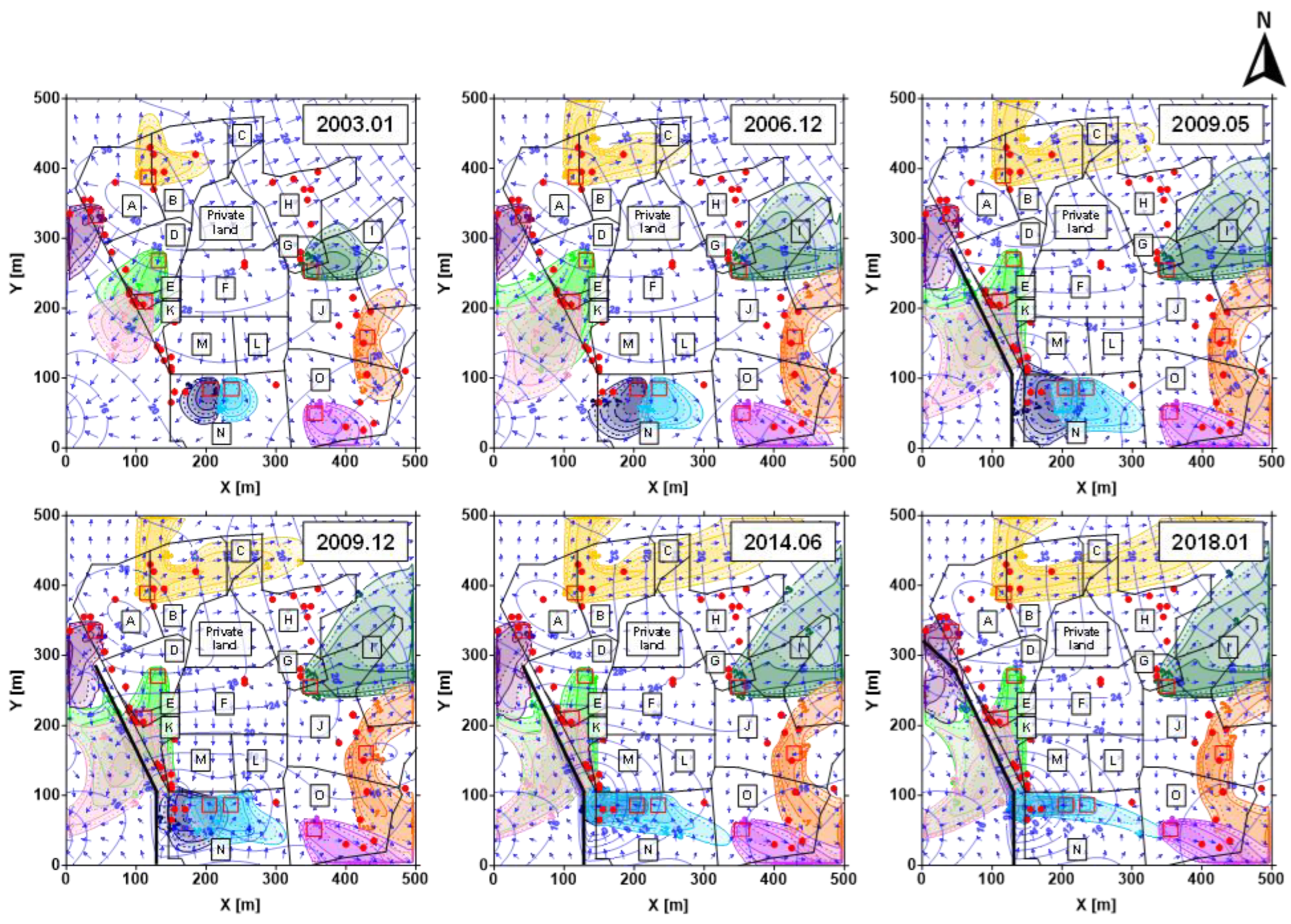
The groundwater flow behaviors of the site can be divided into four main stages, corresponding to changes in the boundary conditions induced by the remediation measures: (1) installation of the impermeable wall (March 2007) and the start of pumping (September 2007), (2) operation of pumping aeration treatment in area N (July 2009), (3) start of pumping in the entire area as remediation measure of 1,4-dioxane contamination (April 2013), and (4) extension of the impermeable wall (July 2014). Based on a comparison of the groundwater level distribution and the spreading behavior of the contamination plume shown in Figure 3, the site-wide spreading behavior as a function of changes in the groundwater level distribution can be interpreted as follows.

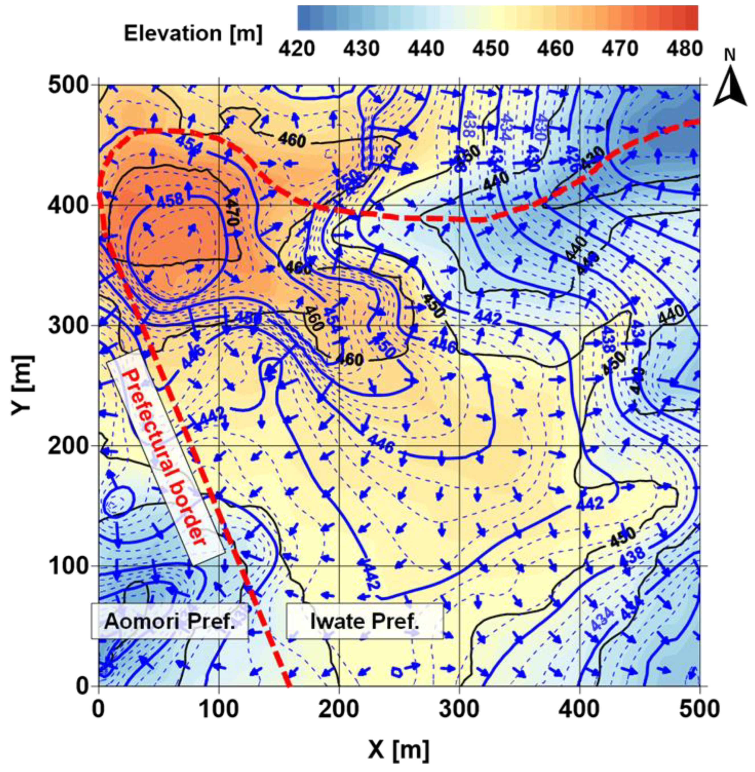
(1) The spread of the contamination plumes through December 2006 is due to the initial distribution of groundwater levels. Groundwater flows primarily in two directions: to the southwest and to the northeast, bounded by a watershed that crosses the site from northwest to southeast. Accordingly, plumes spread to the southwest in Areas A, D, and E; to the northeast in Area G; and to the southeast in Area O. Furthermore, since Area E is downstream of Area D, the plume originating from Area D overlaps with that of Area E. In Areas B, J, and N, however, the plume spreads in two different directions, depending on the local distribution of flow direction within the areas: to the north and east in Area B, to the northeast and southeast in Area J, and to the southwest and southeast in Area N.

(2) The May 2009 distribution shows that with the construction of the impermeable wall and that the start of pumping near the wall, the groundwater flow direction along the impermeable wall in areas D, E, and M changed from southwest to south. The contamination plumes originating from Areas D, E, M, and N overlap near the boundary between Areas M and N. In contrast, the effect of the impermeable wall and pumping on the flow direction in Areas B, G, J, and O is relatively small. Thus, the spreading direction of the contamination plume did not change significantly. In Area A, the plume continued to spread to the southeast because the impermeable wall had not been extended.

(3) In December 2009, when the pumping and aeration treatment was conducted in the N area, a hydraulic gradient toward the inside of the site was generated from the southern boundary of the N area, and the spreading direction of the plume was shifting toward the north. In addition, the influx of groundwater from the outside is expected to have a dilution effect on the 1,4-dioxane concentration at the site. On the other hand, no significant change was observed in the distribution of flow direction or spread of contamination across the site, compared to (2).

(4) In June 2014, after water pumping in the entire area had started, the hydraulic gradient near the boundary between the M and N areas increased with the increase in pumping near the impermeable wall, and the extent of the plume tended to increase in that direction.

(5) In January 2018, after the extension of the impermeable wall, the distribution shows that the flow direction in Area A has changed and the plume has partially spread along the impermeable wall toward the southeast. In addition, in Area O, which is downstream of Area N, the plume originating from Area N partially overlaps with the plume in Area O.

Although the 1,4-dioxane concentrations in Areas F and H were above the standard in May 2010, each well is outside the area where the contamination plume is spreading, as shown in Figure 3. Based on the flow direction distribution as of December 2009, it is difficult to explain why F-2 ($\mathit{x}$ = 255 m and $\mathit{y}$ = 265 m) exceeded the standard, as the range for remediation in area F is $\mathit{x}$ = 190–220 m and $\mathit{y}$ = 230–250 m, as shown in Figure 2. In area F, groundwater flows from the northwest and discharges mainly in the south direction, with some discharging to the northeast. Since the possibility of contamination spreading from private land located north of area F is extremely low, the exceedance of the standard in F-2 can be interpreted to be due to surface contamination in its vicinity, and the contamination plume originating from area F is expected to overlap downstream of area G. In addition, area H exceeded the standard, which is located downstream of both area B and private land. Thus, the possibility of contamination spreading from private land is extremely low. Furthermore, depending on the location of the contamination source in area B, there is a possibility that the contamination plume could reach area H. However, H-1 ($\mathit{x}$ = 295 m, $\mathit{y}$ = 380 m), the most upstream well on the streamline from area B, has maintained below-standard concentrations throughout 2013–2021, unlike other wells in the same area. Therefore, as in Area F, the exceedance of the standard may be due to surface soil contamination in this area, although no implementation of remediation measures was reported in November 2012.

It is usually necessary to consider the spreading of the contamination plume across areas in the matching of 1,4-dioxane concentration changes. However, based on the observed site-wide plume spreading behavior, conducting matching based on the area-specific interpretation of contamination is possible because there is a low possibility of inflow from another area for areas A, F, H, and J. In other areas, however, a gradual matching process is required, taking into account the concentration changes due to the influx of 1,4-dioxane from upstream, for instance, from area A to D and from area D to E. In particular, for areas M and N, the spread of the contamination plume from several directions in the surrounding area must be taken into account.

3.2. History Matching of Spatial-Temporal 1,4-Dioxane Concentration Changes for Area A

We use Area A here as an example to show the progression of changes in 1,4-dioxane concentration in this study because for Area A, the possibility of influx of the 1,4-dioxane from other areas is very low, and the effects of spreading contamination from other areas can be virtually ignored. To establish the boundary conditions for the inflow of 1,4-dioxane into the aquifer, the correlation between the change in the distribution of groundwater flow direction and the effects of the remedial action was first interpreted based on the monitoring results of 1,4-dioxane concentration for each pumping well in Area A and the calculated groundwater level distribution shown in Figure S6.

In A-4 ($\mathit{x}$ = 35 m, $\mathit{y}$ = 340 m), the concentration had been above ten times higher than the environmental standard (0.05 mg/L) for more than three years since the start of monitoring in April 2013. Nevertheless, after the excavation and removal of the contaminated soil near the western boundary in December 2016, a significant decrease in the concentration was confirmed. Therefore, the inflow of 1,4-dioxane into the aquifer after this date is interpreted as a converging trend. Corresponding to this actual result of the remedial action, the area around the western boundary, including A-4, can be considered a source of contamination (source of inflow to the aquifer), which is referred to below as CSA-1. In Area A, an extension of the impermeable wall was constructed in July 2014 to prevent contamination on the side of Aomori Prefecture. The groundwater level distribution shows that before the extension of the impermeable wall in January 2014, groundwater flowed mainly in the southwest direction around A-4 while turning to the A-6 side ($\mathit{x}$ = 5 m, $\mathit{y}$ = 335 m) in the west direction after the extension (January 2015). The concentration at A-6 was 0.018 mg/L in August 2014 but has since increased to above the standard, which could be interpreted because of the change in the flow direction caused by the extension of the impermeable wall, and the contamination plume that spread in the direction of A-6 originated from CSA-1.

On the other hand, the increase in concentration at A-2 ($\mathit{x}$ = 25 m, $\mathit{y}$ = 355 m) after April 2013 is unlikely to have originated from CSA-1, considering its locational relationship with A-4 and the difference in contamination levels between them, in addition to the groundwater flow direction in January 2014, suggesting the existence of another contamination source just near A-2. This contamination source is referred to as CSA-2. In CSA-2, the inflow into the aquifer can be considered to have started around April 2013, corresponding to the trend of an increase in concentration at A-2. In addition, remediation measures by pumping began in August 2015 at A-5 ($\mathit{x}$ = 35 m, $\mathit{y}$ = 355 m), which is located immediately adjacent to A-2. The distribution of groundwater levels since pumping began shows the formation of a hydraulic gradient from the surrounding area toward A-5 (January 2016). The decrease in concentration in A-2 since November 2015 is interpreted mainly as a result of remediation measures by pumping. After that, the decrease has become remarkable since January 2017, suggesting that the inflow from CSA-2 has been a converging trend since then.

In A-1 ($\mathit{x}$ = 70 m, $\mathit{y}$ = 380 m), which is the only well located across the watershed in area A. The concentration had already exceeded the standard in April 2013, and although it showed a slight downward trend after 2016, the concentration level remained above the standard. In May 2020, a chemical treatment method was applied in the central area of area A, and a significant decrease in concentration was confirmed after this period. According to the actual results of these remediation measures, the area near the center of area A could be regarded as the third contamination source, referred to as CSA-3. Based on the concentration change in A-1, it is interpreted that the inflow from CSA-3 into the aquifer ceased after May 2020. The distribution of groundwater levels shows that the water level is highest near the center of this area, and the streamlines radiate to the directions of A-2~A-5 in addition to the direction of A-1 on the north side. A-2 is located on the streamline westward from the center. However, the concentration at A-2 was 0.29 mg/L in October 2014, while that at A-1 was 0.12 mg/L. A-2, located downstream of A-1, according to the locational relationship with the central area, showed a higher concentration. Therefore, the presence of CSA-3 is expected to have little effect on the increase in the concentration of A-2. In addition, CSA-3 is expected to be located slightly on the side of A-1 across the watershed, where the spreading of the contamination plume toward A-2 and A-5 will have little effect. In addition, in A-3 ($\mathit{x}$ = 55 m, $\mathit{y}$ = 305 m), a concentration of around 0.01 mg/L although below the environmental standards, has continued to be detected until 2022, possibly due to the spreading of the contamination plume to the south, which originated from CSA-3.

Based on the above discussion, for area A, history matching of 1,4-dioxane concentrations will be performed by placing three contamination sources: CSA-1 (near the western boundary), CSA-2 (just near A-2), and CSA-3 (near the central area). In the matching process, in addition to the locational relationship of the pumping well to each contamination source, the amount of 1,4-dioxane inflow ${\mathit{Q}}_{nwi,\mathbf{1}}$ [kg], area of the contamination source ${\mathit{A}}_{\mathit{c}\mathit{s}}$ [m²], inflow start time $\mathit{S}\mathit{T}$ [years after], and inflow end time $\mathit{E}\mathit{T}$ [years after] described in Equation (3) are treated as parameters. For the inflow end time $\mathit{E}\mathit{T}$, the values could be set based on concentration changes and actual results of the remediation measures, namely, December 2016 for CSA-1 and CSA-2, and May 2020 for CSA-3. The inflow start time $\mathit{S}\mathit{T}$ of CSA-2 was set in April 2013, at which the concentration of A-2 increased. As for CSA-1 and CSA-3, the $\mathit{S}\mathit{T}$ should be set to an earlier time because the concentrations of A-1 and A-4, which are in the vicinity of CSA-1 and CSA-3, had already increased in April 2013. However, it was difficult to determine $\mathit{S}\mathit{T}$ only from the changes in concentrations. On the other hand, a survey conducted in 2009 for the entire site, when 4-dioxane was included as a new environmental criterion, did not detect contamination in Area A. Therefore, the spreading of contamination into the aquifer originating from CSA-1 and CSA-3 could be regarded as occurring after 2009, and $\mathit{S}\mathit{T}$ was assumed to be January 2013 for CSA-1 and January 2012 for CSA-3, respectively. Multiple repeated preliminary analyses were conducted to determine the detailed condition setting of the contamination source area ${\mathit{A}}_{\mathit{c}\mathit{s}}$and its locational relationship with the pumping wells; however, these analyses will not be described here for space limitations. The calculation conditions for this matching process are shown in Table S1. The matching process consists of three steps: Step.1: CSA-1, Step.2: CSA-2, and Step.3: CSA-3, in which the amount of 1,4-dioxane, ${\mathit{Q}}_{nwi,\mathbf{1}}$, at each contamination source is appropriately changed in that order. The details of the history-matching process are described below.

3.2.1. Step 1: Placement of Contamination Source CSA-1 near the Western Boundary of Area A

In the first step, the contamination source CSA-1 was placed near the western boundary of area A. Then, the monitoring results were compared with the calculation results using the concentration changes at A-4 and A-6 as indicators. CSA-1 was placed in the range of $\mathit{x}$ = 25 to 40 m and $\mathit{y}$ = 325 to 340 m, including A-4, with an area ${\mathit{A}}_{\mathit{c}\mathit{s}}$ of 225 m², so as to locate A-6 on the west side of CSA-1, because the flow direction to the southwest near A-4 turned to the west toward A-6 after the impermeable wall was installed. The period of inflow of 1,4-dioxane into the aquifer in CSA-1 was set to four years, from January 2013 to December 2016, when a significant decrease in concentration was observed in A-4 due to excavation removal. The analysis was conducted by changing the amount of 1,4-dioxane inflow, ${\mathit{Q}}_{nwi,\mathbf{1}}$, in four cases: Case-01: 5.00 kg, Case-02: 10.0 kg, Case-03: 20.0 kg, and Case-04: 40.0 kg.

As representative calculation results, Figure 4a shows that the 1,4-dioxane concentration and groundwater level distribution change over time for Case-02, where ${\mathit{Q}}_{nwi,\mathbf{1}}$is 10.0 kg. The location of CSA-1 is shown in the red box in the figure. The July 2013 and January 2014 distributions show that prior to the extension of the impermeable wall, the contamination plume originating from CSA-1 spread in the same direction as groundwater flow in the region, including CSA-1 and its downstream side. After the extension of the impermeable wall, the direction of the plume spreading turned to the west, as shown for January 2015, which corresponds with the westward shift of the flow direction near CSA-1, and an increase in the concentration near A-6 was observed. In addition, the distributions in January 2016 and 2017 show that the plume spread toward A-2 and A-5 north of CSA-1 after pumping at A-5, as a hydraulic gradient formed toward A-5. Between CSA-1 and A-6, the trends of plume spreading to the west are stronger, and the concentration near A-6 remains at a high level. Because the CSA-1 site also includes A-4, the concentration near A-4 will remain high as long as inflow from CSA-1 into the aquifer continues. However, by January 2018, the inflow to the aquifer had ceased; as a result, a significant decrease in concentration near A-4 was recognized. A general downward trend was observed at A-5 due to the dilution effect from groundwater flow in addition to pumping remediation.

Figure 4b compares the calculated concentration changes over time at each pump well determined for cases-01 through 04 with the monitoring results. Corresponding to the changes in concentration distribution shown in Figure 4a, the concentrations in A-4 remained beyond the environmental standard for four years after January 2013 and decreased significantly with the end of the inflow in December 2016, while the concentrations in A-6 increased after 2013 and decreased after 2018. These calculations reflect well the trend of concentration change shown in the monitoring results. Furthermore, in Case-02, where ${\mathit{Q}}_{nwi,\mathbf{1}}$ is set to 10.0 kg, the concentration in A-4 and A-6 are the closest to the monitoring results. Based on the results of Case-02, to validate the above interpretation that the increase in concentration at A-6 was due to the spreading of the contamination plume originating from CSA-1, we conducted a series of analyses by varying the placement of CSA-1, the inflow period, and the adsorption coefficients.

As shown in Figure 5a, the source placement varied from $\mathit{x}$ = 25 to 40 m and $\mathit{y}$ = 325 to 340 m in Case-02, to $\mathit{x}$ = 20 to 35 m and $\mathit{y}$ = 340 to 355 m on the north side along the district boundary in Case-05, and $\mathit{x}$ = 30 to 45 m and $\mathit{y}$ = 310 to 325 m on the south side along the area boundary in Case-06, finally to $\mathit{x}$ = 35 to 50 m and $\mathit{y}$ = 325 to 340 m further inside the area boundary in Case-07. The analysis was conducted with ${\mathit{Q}}_{nwi,\mathbf{1}}$ and the inflow period set equal to those in Case-02, and the results were compared with the monitoring results using A-4 and A-6 as indicators, as shown in Figure 5b.

In Case 05, the contamination plume reached the site of A-6 earlier due to the southwestern groundwater flow before the extension of the impermeable wall, and the trend of the concentration increase after 2013 is significant; with the change of the dispersion direction of the plume due to the change of the flow direction after the extension, the concentration decrease occurred as early as the second half of 2015, resulting in a significant difference from the monitoring results. In case 06, the concentration increase in A-4 cannot be reproduced because A-4 is not included within the range of CSA-1. In addition, the spreading direction of the contamination plume was different, and the concentration in A-6 remained more than an order of magnitude lower than the monitoring results. In Case-07, the distance between CSA-1 and A-6 was greater than in Case-02, and the timing of the concentration increase was delayed due to the delay in the arrival of the contamination plume at the position of A-6. Based on the above results from Case-05 to Case-07, the placement of CSA-1 in Case-02 is considered appropriate. This supports the interpretation that the increase in concentration at A-6 is due to the spread of the contamination plume originating from CSA-1.

To verify the inflow period, Cases 08~10 were tested with CSA-1 and ${\mathit{Q}}_{nwi,\mathbf{1}}$ equal to those in Case-02. In Case-08, Case-09, and Case-10, the period of inflow was set from January 2011 to December 2016 (6 years), from January 2015 to December 2018 (4 years), and from January 2013 to December 2014 (2 years), respectively. Case-08 assumes an early spreading of contamination, Case-09 assumes a later spreading, and Case-10 assumes an early excavation removal compared to Case-02 (January 2013 to December 2016). The obtained results in the different cases of the period of inflow are shown in Figure 6 and are compared with the monitoring data using A-4 and A-6 as indicators.

In Case-08, the concentration of A-6 had already exceeded the standard in early 2012, which is different from the monitoring results. In Case-09, the concentration changes to exceed the standard in the two years by 2015 could not be well reproduced in either well. In addition, because the inflow of 1,4-dioxane to the aquifer continued after December 2016, there was a delay in the decrease in concentration, resulting in a significant difference from the monitoring results. In Case 10, since the inflow to the aquifer stopped after January 2016 due to excavation and removal, it is impossible to reproduce the concentration changes that have been above the standard since 2016. Based on the above results for Cases 08 through 10, under the assumption that the placement of CSA-1 is appropriate, the condition of four years of inflow from January 2013 through December 2016 can be considered appropriate, indicating that the spread of contamination into the aquifer originating from CSA-1 occurred relatively recently.

Furthermore, as described in Section 2.2 (2), considering the relatively low adsorptive of 1,4-dioxane in the sandy soil, the adsorption coefficient ${\mathit{K}}_{\mathit{d},\mathbf{1}}$ for a series of numerical analyses was set to 1.00 × 10⁴ m³/kg instead of 7.88 × 10⁴ m³/kg that were obtained experimentally. A validation of this ${\mathit{K}}_{\mathit{d},\mathbf{1}}$ value was also conducted using the same 1,4-dioxane inflow condition of Case-02, and the ${\mathit{K}}_{\mathit{d},\mathbf{1}}$ values were changed in four steps, Case-11: 7.88 × 10⁴ m³/kg (corresponding to the experimental value), Case-12: 5.00 × 10⁴ m³/kg, Case-13: 5.00 × 10³ m³/kg and Case-14: 0.00 × 10⁰ m³/kg (without consideration of adsorption) with respect to 1.00 × 10⁴ m³/kg for Case-02, respectively. The results obtained and the comparison with the monitoring results are shown in Figure 7. In cases 11 and 12, 1,4-dioxane had a higher absorption capacity than in case 02, and the amount of 1,4-dioxane retained on the surface of soil particles as the adsorbent increased, resulting in delayed advection and dispersion in the aquifer. As a result, the concentration at A-4 after excavation and removal in January 2017 is declining slowly, and the timing of the concentration increase at A-6 is also delayed. In contrast, in Cases 13 and 14, the amount of 1,4-dioxane absorbed was lower, and the mobility of 1,4-dioxane due to advection and dispersion in the aquifer increased, resulting in a significant decrease in concentration in both wells compared to the monitoring results. The above results suggest that the adsorptive of 1,4-dioxane to the soil is low but has a certain level of adsorptive and that the use of a ${\mathit{K}}_{\mathit{d},\mathbf{1}}$ value of around 1.00 × 10⁴ m³/kg best reproduced the plume spreading behavior caused by advection and dispersion.

Based on the above validity verification of the placement of CSA-1, the inflow period, and the adsorption treatment, a comparison of the calculated and monitored concentration changes at A-1, A-2, A-3, and A-5 is made in Figure 4. Since A-1 and A-3 are independent of changes in groundwater flow direction and are outside the range of contamination plume spreading originating from CSA-1, it is difficult to reproduce the concentration changes in these wells. On the other hand, A-2 and A-5 are not located in the main direction of spreading the contamination plume, so the increase in concentration in these wells can be interpreted as due to pumping at A-5. In particular, at A-2, the difference between the calculated results and the monitoring results in terms of the concentration level and the timing of the concentration increase is so large that the effect of CSA-1 on the concentration increase at A-2 is very small. This result provides a basis for considering CSA-2 as a separate source of contamination from CSA-1 to reproduce the concentration change in A-2. In addition, based on the results of the study in Step 1, the conditions in Case-02 that best reproduce the concentration changes in A-4 and A-6 are used in subsequent Steps 2 and 3 for the conditions related to CSA-1.

3.2.2. Step 2: Placement of Contamination Source CSA-2 to the Vicinity of A-2

In Step 2, CSA-2 is newly placed in addition to CSA-1 in Step 1, using the changes in the concentrations of A-2 and A-5 as indicators to reproduce the monitoring results. A-2 and A-5 are only 10 m apart in the $\mathit{x}$ direction, and both wells were located almost on the same streamline to the west direction with A-5 upstream with respect to A-2 before the start of pumping at A-5. Concentration levels were generally higher in A-2, which was located downstream. Therefore, we performed a series of preliminary analyses to determine the placement of CSA-2 under the condition that CSA-2 should have little effect on the concentration increase of A-5 and should be located just near A-2. As a result, the contamination source area ${\mathit{A}}_{\mathit{c}\mathit{s}}$ is set as 100 m² (10 × 10 m) and is placed in the range of $\mathit{x}$ = 20 to 30 m and $\mathit{y}$ = 360 to 370 m to the north of the vicinity of A-4. The period of inflow of the 1,4-dioxane from CSA-2 into the aquifer was defined as 3.75 years, from April 2013, when the concentration in A-2 started to increase, to December 2016, when a significant decrease in concentration was observed, according to the monitoring results. The analysis was conducted by changing the amount of the 1,4-dioxane inflow ${\mathit{Q}}_{nwi,\mathbf{1}}$ during this period in four steps: Case-15: 1.00 kg, Case-16: 2.00 kg, Case-17: 5.00 kg, and Case-18: 10.0 kg.

As an example of the calculation result, the changes of 1,4-dioxane concentration and groundwater level distributions with time obtained for Case-16 when ${\mathit{Q}}_{nwi,\mathbf{1}}$ was set to 2.00 kg, is shown in Figure 8a. The distributions in July 2013, January 2014, and January 2015 show that before the start of pumping at A-5 in August 2015, there was no significant change in the flow direction near A-2 and A-5 before and after the extension of the impermeable wall; the contamination plume spread mainly toward the southwest side. According to the positional relationship with CSA-2, A-5 is outside the main spreading direction of the plume, and the increase in concentration at A-5 is probably mainly due to dispersion. From the January 2016 distribution, after the start of pumping at A-5, a hydraulic gradient developed from A-2 toward A-5, and the further spreading of the plume was controlled by pumping. Since January 2017, since the inflow from CSA-2 into the aquifer has stopped, concentrations near A-2 and A-5 will decrease over time as pumping continues at A-5. A-1 and A-3 are outside the area where the contamination plume from CSA-2 is spreading, regardless of the change in groundwater flow direction.

Figure 8b compares the monitoring results with the concentration changes over time in each pumping well obtained in Case-15–18. The results from Case-02 are also shown in this figure. Prior to pumping in April 2015, concentrations in A-2 had been gradually increasing since April 2013 and were beyond environmental standards, while concentrations in A-5 remained below standard, although a slight increase was observed. The change in concentration in A-5 during this phase is consistent with the interpretation of the concentration distribution shown in Figure 8a, which is due to the lateral spread of the contamination plume. A significant increase in the concentration in A-5 was observed with the start of pumping, and the concentration in A-4 also increased once, depending on the spatial relationship with CSA-2.

After that, with the end of 1,4-dioxane inflow from CSA-2 to the aquifer in December 2016, the concentrations in both wells showed a decrease. This trend of concentration changes is regardless of ${\mathit{Q}}_{nwi,\mathbf{1}}$, and indicate that the monitoring results have been well reproduced. Especially for Case-16, with ${\mathit{Q}}_{nwi,\mathbf{1}}$ of 2.00 kg, the calculated results show that concentration levels in A-2 and A-5 are closest to the monitoring results. It also confirms that the spreading of the contamination plume originating from CSA-2 has little effect on the concentration change in A-6, which is located downstream. Based on the above results in Step 2, in addition to the conditions obtained in Case-02 for CSA-1, the conditions obtained in Case-16, which best reflect the concentration changes in A-2 and A-5, are adopted in Step 3 for the set of conditions for CSA-2.

3.2.3. Step 3: Placement of Contamination Source CSA-3 near the Center of Area A

In step 3, we performed the analyses with the newly placed CSA-3 in addition to CSA-1 in step 1 and CSA-2, using the concentration changes in A-1 and A-3 as indicators as well. From the monitoring results, after the chemical treatment in the central part of Area A corresponding to CSA-3 was conducted in May 2020, a significant decrease in the concentration in A-1, which is close to CSA-3, was observed. According to the monitoring results and groundwater level distribution shown in Figure S6, based on the interpretation that the presence of CSA-3 has little effect on the concentration change at A-2 and A-5, and the increase in concentration at A-3 is caused by the southward advection and dispersion originating from CSA-3, through multiple repeated preliminary analyses, the CSA-3 area ${\mathit{A}}_{\mathit{c}\mathit{s}}$was set to 400 m² (20 × 20 m) and placed in the range of $\mathit{x}$ = 65 to 85 m and$\mathit{y}$ = 355 to 375 m across the watershed just near A-1. The period of 1,4-dioxane inflow from CSA-3 to the aquifer was assumed to be 8.4 years, from January 2012 to May 2020, when a significant decrease in concentration at A-1 was confirmed by the application of the chemical method. The analyses were conducted by changing the amount of 1,4-dioxane inflow ${\mathit{Q}}_{nwi,\mathbf{1}}$ in four steps: Case-19: 3.00 kg, Case-20: 6.00 kg, Case-21: 12.0 kg, and Case-22: 24.0 kg.

As a representative result, Figure 9a shows the changes in the 1,4-dioxane concentration and groundwater level distribution over time obtained for Case-20 when ${\mathit{Q}}_{nwi,\mathbf{1}}$ is set to 6.00 kg. Before and after the extension of the impermeable wall in July 2014 and the startup of pumping at A-5 in April 2015, the distribution of radial groundwater flow directly from the center of Area A did not change significantly. Accordingly, the area where 1,4-dioxane concentrations increased spread over time. Both A-1 and A-3 were contained in this area in January 2013. This is especially true since the concentration on the north side of CSA-3 is higher, indicating that the contamination plume originating from CSA-3 spreads mainly toward A-1 on the north side.

Figure 9b compares the monitoring results with the concentration changes over time in each of the pump wells obtained in Cases 19 through 22. This figure shows that the concentration in A-1 was beyond environmental standards for eight years beginning in January 2012, and then decreased significantly with the end of inflow to the aquifer in May 2020. In addition, an increase in concentration was observed in A-3 due to the advection and dispersion of 1,4-dioxane over a large area in Area A (see Figure 9a). Compared to Case 16, the increase in A-5 occurred earlier in Cases 19 through 22, and the decrease in concentration in each well after the cessation of 1,4-dioxane inflow from each contamination source was relatively slower. However, the concentrations change at a lower level than the standard. Thus, the effect of advection/dispersion from CSA-3 on the concentration changes in A-2, A-4, A-5, and A-6 can be considered relatively small. These whole behaviors are common regardless of the ${\mathit{Q}}_{nwi,\mathbf{1}}$, and the trend of concentration change obtained from monitoring results is well reproduced. The results of Case-20, with ${\mathit{Q}}_{nwi,\mathbf{1}}$ value of 6.00 kg, showed the best matching with monitoring results for concentration levels in A-1 and A-3.

Based on the results of Steps 1 to 3, the final matching of spatial-temporal changes in 1,4-dioxane concentrations in the aquifer for area A was made based on the calculation conditions of Case-20 slightly by adjusting the amount of 1,4-dioxane inflow ${\mathit{Q}}_{nwi,\mathbf{1}}$ and the inflow period for better reproducing. In the series of analyses, the boundary conditions for the termination of inflow into the aquifer were given based on the actual results of remediation measures. However, since the decrease in concentration in the monitoring results is slower compared to the results of Case-20, it is supposed that the inflow into the aquifer may continue, although only slightly. Therefore, the boundary condition should be newly defined for subsequent inflow. In addition, the distribution of ${\mathit{Q}}_{nwi,\mathbf{1}}$ within each contamination source, and its time variation was also partially considered to better reproduce the concentration changes at each pumping well. Moreover, to reproduce the rapid decrease in concentration just after April 2013 at A-3, CSA-4 was placed as an additional contamination source at $\mathit{x}$ = 55–65 m and $\mathit{y}$ = 305–315 m upstream of A-3. The conditions for the inflow of 1,4-dioxane into the aquifer at each contamination source are shown in

Table 4. The conditions for the inflow of 1,4-dioxane into the aquifer at each contamination source.

Source	Period	${\mathit{Q}}_{nwi,1}$ (kg)
CSA-1	2013.1~2014.12	1.00 (x = 25~40 m, y = 325~335 m)
		4.00 (x = 25~40 m, y = 335~340 m)
	2015.1~2016.12	2.50
	2017.1~2020.12	0.66
CSA-2	2013.7~2016.6	1.50
	2016.7~2022.12	0.30
CSA-3	2012.1~2015.12	4.00
	2016.1~2020.4	2.00
CSA-4	2012.11	0.25

.

Furthermore, we interpreted that the remediation measure to the aquifer, in addition to surface soil by application of chemical treatment, had also been achieved based on the rapid decrease in concentration after May 2020 in A-1 and introduced the attenuation rate by Equation (17) within the range of CSA-3 for better reproducing of concentration change in A-1. The final matching results for area A are shown in Figure 10.

3.3. Validity of the Simulation Results and Evaluation of the Effectiveness of the Impermeable Wall and Pumping

According to the history matching process described in the previous sections and taking into account the major remediation activities conducted since 2014 at the boundaries of Areas A and B, the history matching for the changes in 1,4-dioxane concentrations throughout the area was also conducted by defining the surface contamination sources in other areas. The changes in the 1,4-dioxane concentration, the distribution of groundwater levels, and the results of the history matching for each pumping well are also shown in Figure 11. The contamination plume spread behavior in each area follows the interpretation of Figure 3. Even for the location where multiple contamination plumes occur, such as M-2 ($\mathit{x}$ = 150 m, $\mathit{y}$ = 110 m) and N-1 ($\mathit{x}$ = 150 m, $\mathit{y}$ = 65 m), the changes in the concentrations can be well reproduced.

The measured and calculated amounts of total 1,4-dioxane recovery for the period from April 2013 to March 2014, when total 1,4-dioxane recovery by pumping was recorded, are compared in Figure S7. The measured total recovery in February 2014 was 7.37 kg, while the calculated total recovery was estimated to be 8.64 kg, which generally reflected the trend of increased recovery of 1,4-dioxane by pumping. The calculated results of the distribution of 1,4-dioxane concentrations at the site, at least in April 2013, when pumping began throughout the area, reflect the actual contamination situation, both temporally and spatially. Thus, the reliability of the historical matching was confirmed, and the calculated results were considered fully applicable for quantitative assessment of remedial actions, as well as for prediction of future contamination levels. The amount of 1,4-dioxane inflow ${\mathit{Q}}_{nwi,\mathbf{1}}$ [kg], contamination source area ${\mathit{A}}_{\mathit{c}\mathit{s}}$ [m²], the start time of inflow $\mathit{S}\mathit{T}$ [years after], and the end time of inflow $\mathit{E}\mathit{T}$ [years after] for each contamination source obtained from the history matching for the whole area are listed in Table S2. Based on the specified contamination source parameters listed in Table S2, additional analyses were conducted under the following conditions: (1) no remediation (no installation of an impermeable wall and no pumping) and (2) installation of an impermeable wall only (no pumping). The effectiveness of the impermeable wall in preventing the spread of contamination and pumping out water as a remediation measure is then verified by comparing it to the case with the remediation measures shown in Figure 11. Figure 12 shows the changes over time in 1,4-dioxane inflow and recovery by pumping, 1,4-dioxane remaining in the area, 1,4-dioxane discharged from the boundary, and the area in which the environmental standard is exceeded.

Based on the inflow conditions shown in Table S2, the amount of 1,4-dioxane flowing into the aquifer at the end of 2022 was 174 kg, while the amount recovered by pumping was 85.3 kg, with a recovery ratio of about 49.0%. The remaining amount in the aquifer decreased from a peak of 92.7 kg in September 2014 to 27.4 kg at the end of 2022 due to pumping measures. The area above the standard (0.05 mg/L) was correspondingly reduced from 64,400 m² to 29,150 m², less than half due to remediation measures. 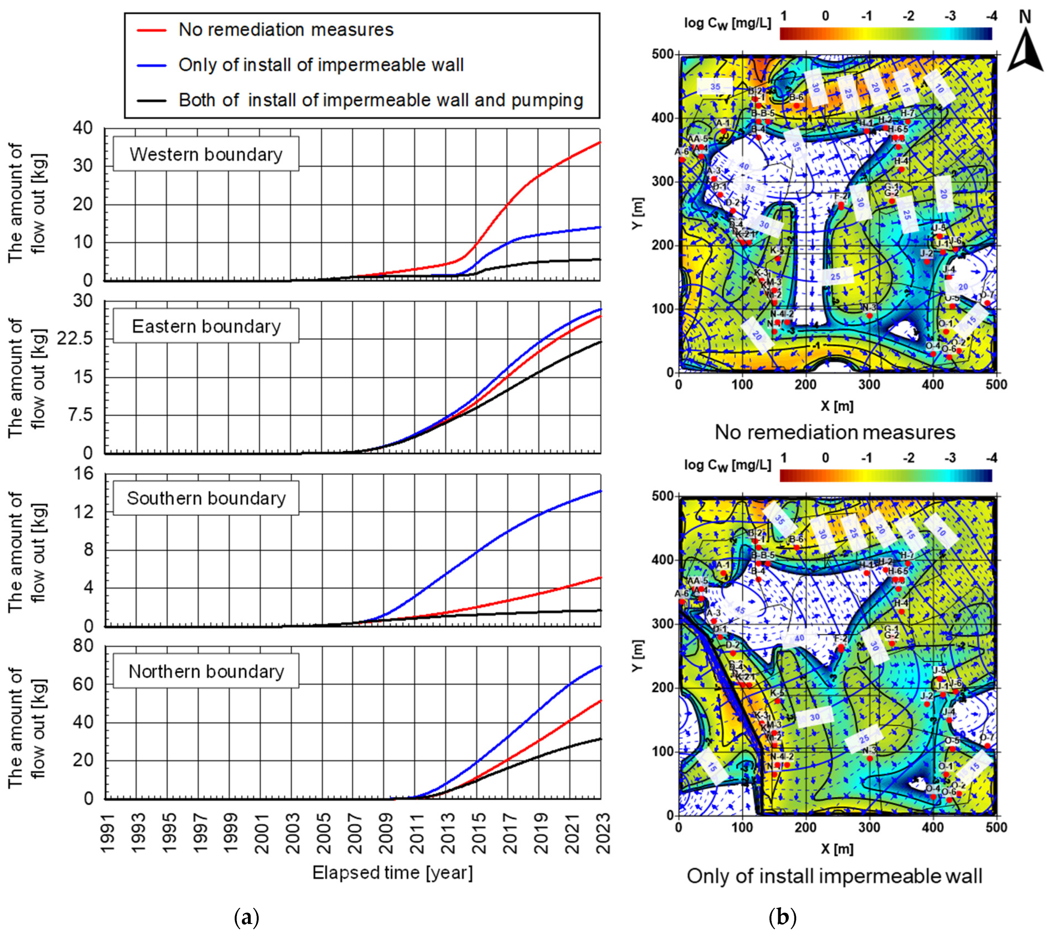In the case without remediation measures, the remaining amount of 1,4-dioxane at the end of 2022 was 56.2 kg, and the area above the standard was 55,650 m². Thus, it was confirmed that the remediation measures have a twice effect on the decrease in the concentration of 1,4-dioxane. However, comparing the case without remediation measures with the case where only the impermeable wall was constructed, the amount of 1,4-dioxane flowing out of the site at the end of 2022 was estimated to be 120 kg and 126 kg, respectively, showing that the construction of the impermeable wall unexpectedly promoted the spreading of 1,4-dioxane and its runoff from the site.

Figure 13a compares the outflow amount at each boundary over time. The amount of runoff on the western boundary decreased from 36.2 kg to 13.8 kg at the end of 2022 due to the installation of an impermeable wall, indicating that the wall was very effective in preventing the spread of contamination to the Aomori Prefecture side. However, at the same time, the discharge on the south side increased from 5.12 kg to 14.2 kg, and on the north side from 51.4 kg to 69.5 kg. The changes in groundwater direction shown in Figure 13b indicate that the installation of the impermeable wall also caused a steep hydraulic gradient in the north and south directions. The installation of an impermeable wall without appropriate pumping measures would unexpectedly accelerate the spread of contamination.

Figure 14 shows the areas that exceed the standard and pose a health risk at the end of 2022 in the case of remediation measures. For health risk determination, groundwater was assumed to be consumed as drinking water, and the daily exposure [mg/kg/day] was calculated by dividing the cumulative exposure $\mathit{E}{\mathit{C}}_{w,\mathbf{1}}$ [mg] by the exposure time, 32 years ($\mathit{E}\mathit{T}\mathit{i}\mathit{m}\mathit{e}$ = 11,680 days), and body weight $\mathit{B}\mathit{W}\mathit{e}\mathit{i}\mathit{g}\mathit{h}\mathit{t}$ [kg]. In Japan, there is no standard value for chronic toxicity, and 0.05 mg/L corresponding to the environmental standard is taken as a temporary reference value. Therefore, the daily exposure amount per 1 kg of body weight is divided by the oral reference dose ($\mathit{O}\mathit{R}\mathit{f}{\mathit{D}}_{\mathbf{1}}$ [mg/kg/day]) according to the U.S. EPA [33], which is defined as the risk level, and when the risk level exceeds 1, it is judged as risky according to the following formula.

$$\mathrm{Risk} \mathrm{level}=\frac{E{C}_{\mathrm{w},1}}{BWeight\times ETime}/ORf{D}_1$$

(17)

Here, the $\mathit{O}\mathit{R}\mathit{f}{\mathit{D}}_{\mathbf{1}}$ value of 1,4-dioxane is 1.60 × 10⁻² mg/kg/day, and the $\mathit{B}\mathit{W}\mathit{e}\mathit{i}\mathit{g}\mathit{h}\mathit{t}$ and daily water intake are set to 50 kg and 2 L/day, respectively, according to the Ministry of Health, Labor and Welfare and Environment Agency (Japan) [34]. As the figure shows, almost the entire area within the site has been remediated below the environmental standard by the end of 2022. In addition, it has been reported by Iwate Prefecture that the areas on the north side of Areas A and B and the off-site areas on the east side of Areas I and J have also exceeded the standard. Although not included in this analysis, Iwate Prefecture has taken additional measures to promote remediation. In addition, the area identified as having risk was limited to Area B and its north side, and even for areas exceeding the standard, the health risk was judged to be generally low, confirming the fact that the remediation measures taken by Iwate Prefecture were sufficient.

The history matching results using the developed model show good agreement with monitoring results, indicating this modeling process can be applied for the prediction of contaminant transport phenomena in groundwater at the site with multiple sources, and the source conditions change with remediation measures, which is a more realistic condition for most illegal dumping sites. This modeling process can also be used in the assessment of the effect of remediation measures and the planning of effective remediation. Furthermore, we supposed that the detailed process provided in this study would be effective for other researchers to follow when dealing with similar illegal dumping sites elsewhere.

4. Conclusions

In this study, an effective numerical model for predicting contamination was developed based on a review of groundwater flow direction distributions caused by remedial actions, that is, the construction of impermeable walls and pumping operations. The simulation first identified the most likely multiple sources of contamination, including the location, inflow volume, and period of each contamination source in the illicit waste site, as well as the adsorption coefficients. Based on this, the historically monitored spatial-temporal 1,4-dioxane concentration changes in the aquifer of the site from the past to the present (1991–2022) were precisely reproduced through historical matching.

Using this model, based on the reproduced contamination situation, future contamination was predicted, and remediation measures were quantitatively evaluated. The construction of impermeable walls and the pumping measures implemented by Iwate Prefecture have been shown to have a two-fold effect on the decrease of 1,4-dioxane concentrations, so the health risk to the target area at the end of 2022 is generally low. However, the study also showed that the installation of the impermeable wall, while having some effect on suppressing the dispersion of 1,4-dioxane in a particular direction, may result in a change in the hydraulic gradient and likely accelerate the overall spreading of 1,4-dioxane from the site if not properly pumped. The development modeling process is also expected to be applicable to another illegal dump site.

References

1. Niyobuhungiro, R.V.; Schenck, C.J. The dynamics of indiscriminate/ illegal dumping of waste in Fisantekraal, Cape Town, South Africa. J. Environ. Manag. 2021, 293, 112954. [Google Scholar] [CrossRef]
2. Otwong, A.; Jongmeewasin, S.; Phenrat, T. Legal obstacles for the circular economy in Thailand: Illegal dumping of recyclable hazardous industrial waste. J. Clean. Prod. 2021, 302, 126969. [Google Scholar] [CrossRef]
3. da Paz, D.H.F.; Lafayette, K.P.V.; de Oliveira Holanda, M.J.; do Carmo Martins Sobral, M.; do Carmo Martins Sobral, L.A.R. Assessment of environmental impact risks arising from the illegal dumping of construction waste in Brazil. Environ. Dev. Sustain. 2020, 22, 2289–2304. [Google Scholar] [CrossRef]
4. Vitali, M.; Castellani, F.; Fragassi, G.; Mascitelli, A.; Martellucci, C.; Diletti, G.; Scamosci, E.; Astolfi, M.L.; Fabiani, L.; Mastrantonio, R.; et al. Environmental status of an Italian site highly polluted by illegal dumping of industrial wastes: The situation 15 years after the judicial intervention. Sci. Total Environ. 2021, 762, 144100. [Google Scholar] [CrossRef] [PubMed]
5. Di Fiore, V.; Cavuoto, G.; Punzo, M.; Tarallo, D.; Casazza, M.; Guarriello, S.M.; Lega, M. Integrated hierarchical geo-environmental survey strategy applied to the detection and investigation of an illegal landfill: A case study in the Campania Region (Southern Italy). For. Sci. Int. 2017, 279, 96–105. [Google Scholar] [CrossRef]
6. Vrijheid, M. Health effects of residence near hazardous waste landfill sites: A review of epidemiologic literature. Environ. Health Perspect. 2000, 108 (Suppl. S1), 101–112. [Google Scholar] [CrossRef] [PubMed] [Green Version]
7. Allen, A. Containment landfills: The myth of sustainability. Eng. Geol. 2001, 60, 3–19. [Google Scholar] [CrossRef]
8. Ritter, L.; Solomon, K.; Sibley, P.; Hall, K.; Keen, P.; Mattu, G.; Linton, B. Sources, Pathways, and Relative Risks of Contaminants in Surface Water and Groundwater: A Perspective Prepared for the Walkerton Inquiry. J. Toxicol. Environ. Health 2002, 65, 1–142. [Google Scholar] [CrossRef]
9. Navarro, J.; Grémillet, D.; Afán, I.; Ramirez, F.; Bouten, W.; Forero, M. Feathered Detectives: Real-Time GPS Tracking of Scavenging Gulls Pinpoints Illegal Waste Dumping. PLoS ONE 2016, 11, e0159974. [Google Scholar] [CrossRef] [Green Version]
10. Đidelija, M.; Kulo, N.; Mulahusić, A.; Tuno, N.; Topoljak, J. Segmentation scale parameter influence on the accuracy of detecting illegal landfills on satellite imagery. A case study for Novo Sarajevo. Ecol. Inform. 2022, 70, 101755. [Google Scholar] [CrossRef]
11. Karimi, N.; Ng, K.T.W.; Richter, A. Development and application of an analytical framework for mapping probable illegal dumping sites using nighttime light imagery and various remote sensing indices. Waste Manag. 2022, 143, 195–205. [Google Scholar] [CrossRef] [PubMed]
12. U.S. EPA. Engineering Issue Paper: In-Situ Chemical Oxidation. 2006. Available online: https://clu-in.org/download/contaminantfocus/pcb/ISCO-600R06072.pdf (accessed on 26 December 2022).
13. U.S. EPA. Remedial Technology Fact Sheet-Activated Carbon-Based Technology for In-Situ Remediation. 2018. Available online: https://semspub.epa.gov/work/HQ/100001159.pdf (accessed on 1 February 2023).
14. O’Connor, D.; Müller-Grabherr, D.; Hou, D. Strengthening social-environmental management at contaminated sites to bolster Green and Sustainable Remediation via a survey. Chemosphere 2019, 225, 295–303. [Google Scholar] [CrossRef] [PubMed]
15. Smith, L.M.; Collins, B. Sustainable remediation column–Experts’ perspectives on the past and future of the practice. Rem. J. 2021, 31, 123–125. [Google Scholar] [CrossRef]
16. Atlabachew, A.; Shu, L.; Wu, P.; Zhang, Y.; Xu, Y. Numerical modeling of solute transport in a sand tank physical model under varying hydraulic gradient and hydrological stresses. Hydrogeol. J. 2018, 26, 2089–2113. [Google Scholar] [CrossRef]
17. Hem, R.; Furuichi, T.; Ishii, K.; Weng, Y.-C. A New Approach for Prediction of 1,4-Dioxane Distribution in Groundwater at an Illegal Dumping Site in Japan. J. Jpn. Soc. Civ. Eng. 2013, 69, II_247–II_258. [Google Scholar] [CrossRef] [Green Version]
18. Banejad, H.; Mohebzadeh, H.; Ghobadi, M.H.; Heydari, M. Numerical simulation of groundwater flow and contamination transport in Nahavand plain aquifer, west of Iran. J. Geol. Soc. India 2014, 83, 83–92. [Google Scholar] [CrossRef]
19. Usoh, A.G.; Ahaneku, I.E.; Horsfall, I.T.; Uwadiegwu Alaneme, G.; Hogan Itam, D. Numerical modeling and simulation of leachate transport in MSW contaminated soil: Impact on seasonal changes. Clean. Mater. 2022, 4, 100089. [Google Scholar] [CrossRef]
20. Xu, T.; Gómez-Hernández, J.J.; Chen, Z.; Lu, C. A comparison between ES-MDA and restart EnKF for the purpose of the simultaneous identification of a contaminant source and hydraulic conductivity. J. Hydrol. 2021, 595, 125681. [Google Scholar] [CrossRef]
21. Xing, Z.; Qu, R.; Zhao, Y.; Fu, Q.; Ji, Y.; Lu, W. Identifying the release history of a groundwater contaminant source based on an ensemble surrogate model. J. Hydrol. 2019, 572, 501–516. [Google Scholar] [CrossRef]
22. Iguro, C.; Furuichi, T.; Ishii, K.; Kim, S. Prediction of 1,4-Dioxane Dispersion Based on Change in Groundwater Flow After Remedial Measures by Three-Dimensional Numerical Simulation—Toward a Permanent Measure for Aomori-Iwate Illegal Dumping Site. J. Jpn. Soc. Civ. Eng. 2012, 68, II_265–II_272. [Google Scholar] [CrossRef]
23. Inoue, D.; Tsunoda, T.; Sawada, K.; Yamamoto, N.; Saito, Y.; Sei, K.; Ike, M. 1,4-Dioxane degradation potential of members of the genera Pseudonocardia and Rhodococcus. Biodegradation 2016, 27, 277–286. [Google Scholar] [CrossRef] [PubMed]
24. Pugazhendi, A.; Rajesh Banu, J.; Dhavamani, J.; Yeom, I.T. Biodegradation of 1,4-dioxane by Rhodanobacter AYS5 and the role of additional substrates. Ann. Microbiol. 2015, 65, 2201–2208. [Google Scholar] [CrossRef]
25. Pongritsakda, T.; Nakamura, K.; Wang, J.; Watanabe, N.; Komai, T. Prediction and Remediation of Groundwater Pollution in a Dynamic and Complex Hydrologic Environment of an Illegal Waste Dumping Site. Appl. Sci. 2021, 11, 9229. [Google Scholar] [CrossRef]
26. Kondo, M.; Sakamoto, Y.; Kawabe, Y.; Nakamura, K.; Watanabe, N.; Komai, T. Development of a Model for Predicting the Volatilization Flux from Unsaturated Soil Contaminated by Volatile Chemical Substances. Environ. Model. Assess. 2022, 27, 251–273. [Google Scholar] [CrossRef]
27. Nakamura, K.; Ito, H.; Kawabe, Y.; Komai, T. Study on Partitioning and Distribution in soil-water phases for 1,4-Dioxane in Geo-Environment. JSCE Trans. G Environ. 2018, 74, 59–66. [Google Scholar] [CrossRef] [Green Version]
28. U.S. EPA. Technical Fact Sheet-1,4-Dioxane. 2017. Available online: https://www.epa.gov/sites/default/files/2014-03/documents/ffrro_factsheet_contaminant_14-dioxane_january2014_final.pdf (accessed on 1 February 2023).
29. Otto, M.; Nagaraja, S. Treatment technologies for 1,4-Dioxane: Fundamentals and field applications. Rem. J. 2007, 17, 81–88. [Google Scholar] [CrossRef]
30. Bruand, A.; Hartmann, C.; Lesturgez, G. Physical Properties of Tropical Sandy Soils: A Large Range of Behaviours. 2005. Available online: https://www.semanticscholar.org/paper/Physical-properties-of-tropical-sandy-soils-%3A-a-of-Bruand-Hartmann/6cdfb65669f9ba1a140d16e9a1b3231b7fc2af6c (accessed on 1 February 2023).
31. Huang, J.; Hartemink, A.E. Soil and environmental issues in sandy soils. Earth-Sci. Rev. 2020, 208, 103295. [Google Scholar] [CrossRef]
32. Koizumi, T.; Shinto, A.; Tsuchida, T.; Yamamoto, S.; Ozasa, H.; Yamada, K.; Kohisa, Y. Experiments and Discussion on Permeability at Steel Sheet Pile Joints. In Proceedings of the The 56th Annual Academic Conference of Japan Society of Civil Engineers, VII-019, Kumamoto, Japan, 2 October 2001. [Google Scholar]
33. U.S. EPA. Risk Assessment Guidance for Superfund Volume I- Human Health Evaluation Manual (Part B Development of Risk-based Preliminary Remediation Goals). 1991. Available online: https://semspub.epa.gov/work/HQ/156739.pdf (accessed on 1 February 2023).
34. Ministry of Health Labour and Welfare. Japan. Safety Data Sheet of 1,4-Dioxane. 2002. Available online: https://anzeninfo.mhlw.go.jp/anzen/gmsds/123-91-1.html (accessed on 1 February 2023).
Figure 1. Elevation contour of dumping site and potential groundwater flow; red dashed line shows the boundary between two prefectures, black line shows the elevation contour, blue line shows the reproduced groundwater distribution based on the survey from 2001 to 2002.
Sustainability 15 03930 g001
Figure 2. Areas where VOC concentrations exceeded soil and groundwater standards in July 2010 and areas where remediation measures were implemented until November 2012.
Sustainability 15 03930 g002
Figure 3. The potential distribution of contamination sources (shown as red boxes) at the site from 1999–2022. The distributions of contaminants from different contamination sources are shown in different colors, and the blue arrows show groundwater flow directions.
Sustainability 15 03930 g003
Figure 4. (a) 1,4-dioxane concentration and groundwater level distribution changes over time for Case-02; (b) comparison of the calculated concentration changes over time at each pumping well with the monitoring results (Cases-01, 02, 03, and 04).
Sustainability 15 03930 g004
Figure 5. (a) The placement of contamination sources in the A-area and (b) the verification of the placement of contamination source by comparing the calculation results with monitoring results (Cases-02, 05, 06, and 07).
Sustainability 15 03930 g005
Figure 6. Comparison of calculated and monitored results for verification of the discharge period from contamination source in the A-area (Cases-02, 08, 09, and 10).
Sustainability 15 03930 g006
Figure 7. Comparison of calculated and monitored results for verification of adsorption coefficient 1,4-dioxine in the A-area (Cases-02, 11–14).
Sustainability 15 03930 g007
Figure 8. Verification of the second source. (a) 1,4-dioxane concentration and groundwater level distribution changes over time for Case–16; (b) comparison of the calculated concentration changes over time at each pumping well with the monitoring results (Cases–01, 15–18).
Sustainability 15 03930 g008
Figure 9. Verification of the third source. (a) 1,4-dioxane concentration and groundwater level distribution changes over time for Case-16; (b) comparison of the calculated concentration changes over time at each pumping well with the monitoring results (Cases-01, 15–18).
Sustainability 15 03930 g009
Figure 10. The final matching results for area A. Comparison of the calculated concentration changes over time at each pumping well for Case 20 with the monitoring results.
Sustainability 15 03930 g010
Figure 11. Comprehensive reproduction results of Iwate site and simulation of contaminated situation from 2010 to 2022. (a) simulation of distribution of 1,4-dioxane in groundwater (2003–2022); (b)The final matching results of whole area of the dumping site between simulation results and remediation measures.
Sustainability 15 03930 g011
Figure 12. (a) The changes in the amounts of 1,4-dioxane inflow and recovery by pumping over time, (b) the remaining 1,4-dioxane in the area, (c) discharged 1,4-dioxane from the boundary, and (d) area exceeding the environmental standard over time, calculated using the source parameters shown in Table S2.
Sustainability 15 03930 g012
Figure 13. (a) Comparison of the outflow 1,4-dioxane amount at each boundary over time, and (b) the groundwater direction and 1,4-dioxane distributions over time.
Sustainability 15 03930 g013
Figure 14. The areas that exceed the standard and pose health risk at the end of 2022 in the case of remediation measures. Red points refer to pumping wells, yellow area is where 1,4-dioxane exceeds the standard (0.05 mg/L) and red area is the high-risk area.
Sustainability 15 03930 g014