Research on Logistics Path Optimization for a Two-Stage Collaborative Delivery System Using Vehicles and UAVs

Abstract

A two-stage planning model for the carrier–vehicle problem with drone (CVP-D) is established in this paper, with the objective of minimizing the delivery time of the drone and the distance traveled by the truck while considering the impact of payload on the drone flight distance. Firstly, based on the customer coordinates, an improved K-Means ++ clustering algorithm is designed to plan the vehicle stopping points, and the vehicle departs from the warehouse to traverse all stopping points in order. Based on the vehicle stopping points, a multi-chromosome genetic algorithm is designed to optimize the vehicle driving path. Then, the drone route is optimized without considering the no-fly zone. Finally, the real data of Jiangsu Province are introduced as a case study to calculate the cost and total time required before and after improvement. The results showed an approximate savings of 16% in time and 19% in cost.

1. Introduction

With the improvement of technology and the widespread use of 5G networks, UAVs (Unmanned Aerial Vehicles) have been applied in various fields. This paper takes vehicle–drone collaborative participation in terminal logistics distribution as the research object, focusing on the hybrid distribution mode route optimization problem. When calculating a group of customer points to be distributed, how to plan the distribution order and distribution path of customer points, how much distribution time can be reduced or how much distribution cost can be reduced are the problems to be solved in vehicle–drone collaborative distribution route schemes faced by logistics enterprises and provide a certain reference basis for subsequent scientific research. The joint distribution diagram of “vehicle + drone” is shown in Figure 1.

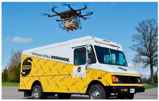
Figure 1. Schematic diagram of joint distribution of “vehicle + drone”.

First, the problem can be divided into two categories according to whether vehicles participate in the distribution process, and then the above two categories can be divided into four categories according to the form of vehicle–drone distribution: First, traveling salesman problem with drones (TSP-D); Second, the vehicle routing problems associated with drones (VRP-D); Third, drone delivery problem (DDP); Fourth, vehicle support drone delivery problem (CVP-D). The classification diagram is shown in Figure 2.

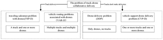
Figure 2. Types of truck–drone collaborative distribution modes.

Murray and Chu introduced the vehicle routing problem of a combination of trucks and drones. In this paper, the authors proposed two new variants of the traditional Traveling Salesman Problem (TSP), named the Flying Partner Traveling Salesman Problem (FSTSP) and the Parallel UAV Dispatch Vehicle Routing Problem (PDSTSP) [1]. Agatz et al. proposed two heuristic algorithms based on local search and dynamic programming for solving the TSP-D problem, which is very similar to the FSTSP proposed by Murray and Chu [2]. These authors confirmed the findings of Ferandez et al., that drones must be twice as fast as trucks [3]. Several authors have proposed algorithms to address the problems raised by Murray and Chu [1] and Agatz et al. [2]. These two papers serve as the basis for several TSP-D variant questions. Yurek and Ozmutlu [4], Ponzal [5], Freitas and Penna [6], Mbiadou Saleu et al. [7] and Bouman et al. [8] proposed several algorithms for these problems. Carlsson and Song analyzed the benefits of using single-truck and single-drone delivery systems and described how much improvement can be achieved by introducing drones to deliver packages. In their model, drones can take off from various points, not limited to the customer’s location [9]. Poikonen et al. [10] proposed four branch- and-bound based heuristics for the TSP-D variant of Agatz et al. [2]. In their computational study, they compared the effectiveness and efficiency of four heuristic methods, analyzing the tradeoff between the target value and the computation time. Phan et al. [11] extended the work of Ha et al. [12] by considering a modified version of their GRASP to address a variant of TSP-D called multi-drone TSP. Salama and Srinivas proposed a mathematical planning model to jointly optimize customer clustering and truck and drone routing [13]. Moshref-Javadi et al. [14,15], Chang and Lee [16] and Muray and Raj also considered the path planning problem of multiple UAVs. Anees Abu-Monshar [17,18] by considering different start/end locations, capacities, as well as shifts in the Time Window variant, proposed to capture the uniqueness of vehicles by modelling them as agents while governing the search with centralized agent cooperation. In summary, the advantages and disadvantages of the heuristic algorithms mentioned above are shown in Table 1.

Table 1. Algorithm summary.

Algorithm Type	Algorithm Name	Advantage	Disadvantage
Deterministic algorithm	Dijkstra	Strong seeking ability	Slow solving speed
	A*	Fast solving speed	High computational complexity
	D*	① Good real-time ② Dynamic obstacle avoidance	Not adapted to complex maps
	Jump search algorithm	① Fast solving speed ② Algorithm has simple structure	Applies only to maps with no grid weight differences
Stochastic algorithm	Genetic algorithm	① Wide applicability ② Multi-population co-evolution	Not adapted to complex maps
	Ant colony algorithm	① Simple and easy to implement ② Multi-population co-evolution	Slow solving speed

The research on collaborative distribution between vehicles and UAVs is now in its early stages, and the following issues still exist. The challenge of vehicle–UAV collaborative distribution is a new problem distinct from the conventional vehicle routing problem, and there are few research achievements in the direction of vehicle–UAV combined distribution mode. The truck–drone cooperative distribution mode cannot be solved using the vehicle routing problem algorithm. The results of the current research lack a comparison analysis and validity verification of various algorithms.

In conclusion, this study optimizes the routes of UAVs and automobiles using the K-Means algorithm and the genetic algorithm, respectively, and compares the revised method with the original approach based on the CVP-D issue. Actual data to implement a realistic and scientific distribution of the two distribution techniques, a city in Jiangsu Province was introduced. The findings of the solution demonstrate that the enhanced algorithm can swiftly plan a realistic vehicle–UAV cooperative distribution path and raise the vehicle–UAV’s operational efficacy.

2. Problem Description and Model Construction

2.1. Problem Description

As shown in Figure 3, the traditional vehicle transport mode sets out with all the customers’ parcels, distributes them in turn according to the set route and finally returns to the warehouse. However, traditional vehicles find it challenging to move or arrive in locations with traffic jams and challenging terrain; hence, the UAV is chosen for distribution. Due to power and load limitations, UAV cannot handle all distribution jobs even if all regions implement UAV distribution. To cut down on vehicle wait times and maximize the effectiveness of vehicle UAV distribution, joint vehicle and UAV distribution is used. The specific distribution mode is shown in Figure 4. The drone starts delivering the cargo to adjacent clients as soon as the vehicle pulls up to the secondary distribution facility.

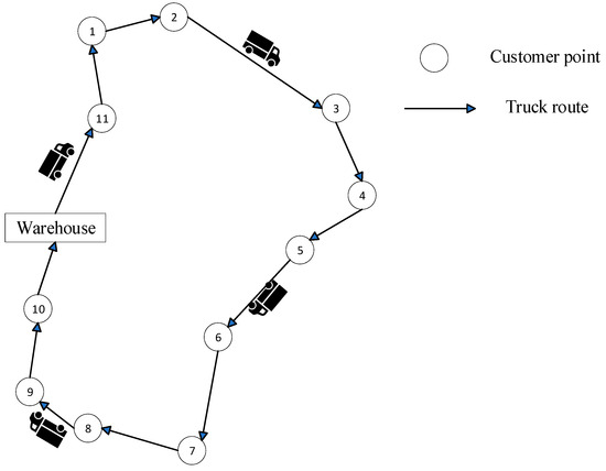
Figure 3. Traditional logistics vehicle distribution organization flow chart.

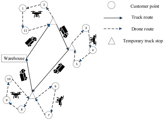
Figure 4. Flow chart of vehicle–drone cooperative distribution organization.

2.2. Model Assumptions

To ensure the generalization and solvability of the model, it is necessary to simplify the model. Relevant assumptions are as follows:

(1)

Only one vehicle and one drone are used in the delivery process;

(2)

All customer points need to be delivered only once;

(3)

Consider the time it takes for the UAV to load and unload packages on the vehicle and change batteries;

(4)

The duration of the UAV staying at the customer’s point is not considered;

(5)

The flying speed of the UAV is constant;

(6)

The UAV can only take off and land when the vehicle arrives at the docking point and shall not take off while the vehicle is in operation;

(7)

Vehicles can only park at temporary parking points, not at customer parking points.

2.3. Model Building

2.3.1. Model Notion

The notation involved in this model is shown in Table 2.

Table 2. Model notation description table.

Notation	Notation Description
$\mathrm{D}=\left\{0\right\}$	Warehouse collection
$\mathrm{S}=\left\{\mathrm{1,2},3\cdots \mathrm{n}\right\}$	Set of n service points
$\mathrm{V}=\left\{1+\mathrm{n},2+\mathrm{n},3+\mathrm{n}\cdots \mathrm{m}+\mathrm{n}\right\}$	m + n vehicle temporary stopping point
$\mathrm{K}$	The set of arcs traveled by all vehicle paths
$\mathrm{U}$	The set of arcs traveled by all drone paths
$\mathrm{T}$	Total time
${\mathrm{q}}_{\mathrm{i}}$	Parcel weight of customer i point
${\mathrm{d}}_{\mathrm{i}\mathrm{j}}$	Distance of the vehicle travels from the vehicle temporary stopping point i to j
${\mathrm{x}}_{\mathrm{i}\mathrm{j}}$	Distance of the drone from point i to j
${\mathrm{v}}_{\mathrm{u}}$	Drone speed
${\mathrm{v}}_{\mathrm{v}}$	Truck speed
${\mathrm{D}}_{\mathrm{m}\mathrm{a}\mathrm{x}}$	The longest flight distance of the UAV
${\mathrm{Q}}_{\mathrm{m}\mathrm{a}\mathrm{x}}$	The maximum payload of the drone
${\mathrm{Q}}_{\mathrm{i}\mathrm{j}}$	The drone’s payload leaves from i to j
$\mathsf{\beta }$	Impact factor of drone power consumption
${\mathrm{t}}_{\mathrm{R}}$	Time required for the drone to land on the vehicle and replace the battery
${\mathrm{t}}_{\mathrm{F}}$	Time required for the drone to load on the vehicle and take off from a vehicle
${\mathrm{t}}_{\mathrm{i}}$	The moment the vehicle arrives at point i
${\mathrm{t}}_{\mathrm{i}}^{\prime }$	The moment the vehicle leaves from point i
$\widehat{{\mathrm{t}}_{\mathrm{i}}}$	The moment the drone lands at point i
${\mathrm{e}}_{\mathrm{i}}$	The location of point i in the path of the vehicle
${\mathsf{\epsilon }}_{\mathrm{i}}$	The location of point i in the path of the drone
${\mathrm{B}}_{\mathrm{i}\mathrm{j}}$	The remaining distance the drone can fly from point i to point j
$\mathrm{M}$	An infinite number

To construct a decision, variables ${\mathrm{C}}_{\mathrm{i}\mathrm{j}}$, ${\mathrm{y}}_{\mathrm{i}\mathrm{j}\mathrm{k}}$, ${\mathrm{Z}}_{\mathrm{i}\mathrm{j}\mathrm{k}}$, ${\mathrm{a}}_{\mathrm{i}\mathrm{j}}$ are defined as follows:

$${\mathrm{C}}_{\mathrm{i}\mathrm{j}}=\{\begin{array}{l}1,\mathrm{V}\mathrm{ehicle} \mathrm{travels} \mathrm{from} \mathrm{truck} \mathrm{stop} \mathrm{point} \mathrm{i} \mathrm{to} \mathrm{truck} \mathrm{stop} \mathrm{point} \mathrm{j}\\ 0,\forall \mathrm{i},\mathrm{j}\in \mathrm{V}\end{array}$$

$${\mathrm{y}}_{\mathrm{i}\mathrm{j}\mathrm{k}}=\{\begin{array}{l}1,\mathrm{The} \mathrm{drone} \mathrm{that} \mathrm{takes} \mathrm{off} \mathrm{from} \mathrm{truck} \mathrm{stop} \mathrm{i} \mathrm{flies} \mathrm{to} \mathrm{customer} \mathrm{point} \mathrm{j} \mathrm{and} \\ \mathrm{then} \mathrm{to} \mathrm{customer} \mathrm{point} \mathrm{k}\\ 0,\forall \mathrm{i}\in \mathrm{V},\forall \mathrm{j},\mathrm{k}\in \mathrm{s}\end{array}$$

$${\mathrm{Z}}_{\mathrm{i}\mathrm{j}\mathrm{k}}=\{\begin{array}{l}1,\mathrm{The} \mathrm{drone} \mathrm{flies} \mathrm{from} \mathrm{customer} \mathrm{point} \mathrm{s} \mathrm{back} \mathrm{to} \mathrm{truck} \mathrm{stop} \mathrm{j} \mathrm{and}\\ \mathrm{then} \mathrm{to} \mathrm{customer} \mathrm{point} \mathrm{m}\\ 0,\forall \mathrm{i},\mathrm{k}\in \mathrm{s},\forall \mathrm{j}\in \mathrm{V}\end{array}$$

$${\mathrm{a}}_{\mathrm{i}\mathrm{j}}=\{\begin{array}{l}1,\mathrm{The} \mathrm{trucks} \mathrm{visit} \mathrm{truck} \mathrm{stop} \mathrm{i} \mathrm{and} \mathrm{then} \mathrm{visit} \mathrm{truck} \mathrm{stop} \mathrm{j}\\ 0,\forall \mathrm{i},\mathrm{j}\in \mathrm{D}\cup \mathrm{V}\end{array}$$

The flight distance of UAV has a linear relationship with its load, as shown in Formula (1):

$$d=d_0-\beta \cdot q$$

(1)

2.3.2. Constraint Conditions

The objective function T is established according to the above problem description and symbol description. T represents the total time of vehicle–drone cooperation in delivering packages to all customer points and returning to the warehouse. The time includes three parts, namely, vehicle traveling time, UAV flight time and vehicle waiting time, and the goal is to minimize the total time. The function expression is shown in (2):

$$\min \mathrm{T}={\displaystyle \sum _{\mathrm{i}\in \mathrm{D}\cup \mathrm{V}}{\displaystyle \sum _{\mathrm{j}\in \mathrm{D}\cup \mathrm{V}}\frac{{\mathrm{d}}_{\mathrm{i}\mathrm{j}}}{{\mathrm{V}}_{\mathrm{v}}}}}+{\displaystyle \sum _{\mathrm{i}\in \mathrm{S}}{\displaystyle \sum _{\mathrm{j}\in \mathrm{S}}\frac{x_{\mathrm{i}\mathrm{j}}}{{\mathrm{V}}_{\mathrm{u}}}}}+{\displaystyle \sum _{\mathrm{i}\in \mathrm{V}}{\displaystyle \sum _{\mathrm{j}\in \mathrm{S}}{\displaystyle \sum _{\mathrm{k}\in \mathrm{V}}{\mathrm{Z}}_{\mathrm{i}\mathrm{j}\mathrm{k}}}}}({\mathrm{t}}_{\mathrm{R}}+{\mathrm{t}}_{\mathrm{F}})$$

(2)

The constraints are as follows:

$${\displaystyle \sum _{\mathrm{i}\in \mathrm{V}}{\mathrm{C}}_{\mathrm{i}0}}={\displaystyle \sum _{\mathrm{i}\in \mathrm{V}}{\mathrm{C}}_{0\mathrm{i}}}=1$$

(3)

$$\sum _{\mathrm{i}\in \mathrm{D}\cup \mathrm{V},\mathrm{j}\in \mathrm{D}\cup \mathrm{V}}{\mathrm{C}}_{\mathrm{i}\mathrm{j}}=\sum _{\mathrm{i}\in \mathrm{D}\cup \mathrm{V},\mathrm{j}\in \mathrm{D}\cup \mathrm{V}}{\mathrm{C}}_{\mathrm{j}\mathrm{i}}$$

(4)

$${\displaystyle \sum _{\mathrm{i}\in \mathrm{V}}{\mathrm{C}}_{\mathrm{i}\mathrm{j}}}=1,\forall \mathrm{j}\in \mathrm{V}\mathrm{a}\mathrm{n}\mathrm{d}\mathrm{i}\ne \mathrm{j}$$

(5)

$${\mathrm{e}}_{\mathrm{j}}-{\mathrm{e}}_{\mathrm{i}}+1\le (\mathrm{m}+2)(1-x_{\mathrm{i}\mathrm{j}}),\forall \mathrm{i},\mathrm{j}\in \mathrm{V}$$

(6)

$$1\le \mathrm{e}\mathrm{i}\le \mathrm{m}+2,\forall \mathrm{i}\in \mathrm{V}$$

(7)

$${\mathrm{e}}_{\mathrm{j}}-{\mathrm{e}}_{\mathrm{i}}\le \mathrm{M}\cdot {\mathrm{a}}_{\mathrm{i}\mathrm{j}},\forall \mathrm{i},\mathrm{j}\in \mathrm{V}$$

(8)

$${\mathrm{e}}_{\mathrm{j}}-{\mathrm{e}}_{\mathrm{i}}\ge \mathrm{M}\cdot ({\mathrm{a}}_{\mathrm{i}\mathrm{j}}-1)+1,\forall \mathrm{i},\mathrm{j}\in \mathrm{V}$$

(9)

$${\displaystyle \sum _{\mathrm{i}\in \mathrm{V}}{\displaystyle \sum _{\mathrm{j}\in \mathrm{S}}{\displaystyle \sum _{\mathrm{k}\in \mathrm{V}\cup \mathrm{S}}{\mathrm{y}}_{\mathrm{i}\mathrm{j}\mathrm{k}}=1}}}$$

(10)

$${\displaystyle \sum _{\mathrm{i}\in \mathrm{V}}{\displaystyle \sum _{\mathrm{j}\in \mathrm{S}}{\displaystyle \sum _{\mathrm{k}\in \mathrm{V}\cup \mathrm{S}}{\mathrm{y}}_{\mathrm{i}\mathrm{k}\mathrm{j}}=1}}}$$

(11)

$${\displaystyle \sum _{\mathrm{i}\in \mathrm{V}}{\displaystyle \sum _{\mathrm{j}\in \mathrm{S}}{\displaystyle \sum _{\mathrm{k}\in \mathrm{V}\cup \mathrm{S}}{\mathrm{y}}_{\mathrm{i}\mathrm{j}\mathrm{k}}=}}}{\displaystyle \sum _{\mathrm{i}\in \mathrm{V}}{\displaystyle \sum _{\mathrm{j}\in \mathrm{S}}{\displaystyle \sum _{\mathrm{k}\in \mathrm{V}\cup \mathrm{S}}{\mathrm{y}}_{\mathrm{i}\mathrm{k}\mathrm{j}}}}}$$

(12)

$${\displaystyle \sum _{\mathrm{j}\in \mathrm{S}}{\mathrm{y}}_{\mathrm{i}\mathrm{j}\mathrm{i}}}\ge {\displaystyle \sum _{\mathrm{h}\in \mathrm{V}}{\mathrm{C}}_{\mathrm{i}\mathrm{h}}},\forall \mathrm{i}\in \mathrm{V}$$

(13)

$$\mathrm{M}\cdot {\displaystyle \sum _{\mathrm{i}\in \mathrm{V}}{\mathrm{C}}_{\mathrm{i}\mathrm{h}}}\ge {\displaystyle \sum _{\mathrm{i}\in \mathrm{V}\cup \mathrm{S}}{\displaystyle \sum _{\mathrm{j}\in \mathrm{S}}{\mathrm{y}}_{\mathrm{i}\mathrm{j}\mathrm{h}}}},\forall \mathrm{h}\in \mathrm{V}$$

(14)

$${\mathrm{\epsilon }}_{\mathrm{i}}-{\mathrm{\epsilon }}_{\mathrm{j}}+1\le (\mathrm{n}+2)(1-{\mathrm{y}}_{\mathrm{i}\mathrm{k}\mathrm{j}}),\forall \mathrm{i}\in \mathrm{V},\forall \mathrm{k},\mathrm{j}\in \mathrm{S}$$

(15)

$$1\le {\mathrm{\epsilon }}_{\mathrm{j}}\le \mathrm{n}+2,\forall \mathrm{j}\in \mathrm{S}$$

(16)

Constraint (3) represents that the vehicle starts from the warehouse and returns to the warehouse. Constraint (4) represents the flow balance constraint of the vehicle. Constraint (5) ensures that the vehicle traverses all vehicle stops. Constraints (6) and (7) represent that the Miller–Tucker–Zemlin (MTZ) method of the vehicle eliminates the subloop constraint. Constraints (8) and (9) restrict the sequence of vehicles accessing vehicle parking points. Constraints (10) and (11) represent that all customer points need to be served. Constraint (12) is the flow balance constraints on UAV. Constraints (13) and (14) represent that the UAV can only take off or land from vehicle parking points. Constraints (14)–(16) are the removal of subloop constraints by the Miller–Tucker–Zemlin (MTZ) method for UAVs.

$${\mathrm{Q}}_{\mathrm{i}\mathrm{j}}\le {\mathrm{Q}}_{\mathrm{i}\mathrm{i}}-{\mathrm{q}}_{\mathrm{j}}\cdot {\mathrm{y}}_{\mathrm{i}\mathrm{j}\mathrm{i}}+{\mathrm{Q}}_{\max }(1-{\mathrm{y}}_{\mathrm{i}\mathrm{j}\mathrm{i}}),\forall \mathrm{i}\in \mathrm{V},\forall \mathrm{j}\in \mathrm{S}$$

(17)

$${\mathrm{Q}}_{\mathrm{i}\mathrm{j}}\ge {\mathrm{Q}}_{\mathrm{i}\mathrm{i}}-{\mathrm{q}}_{\mathrm{j}}\cdot {\mathrm{y}}_{\mathrm{i}\mathrm{j}\mathrm{i}}+{\mathrm{Q}}_{\max }(1-{\mathrm{y}}_{\mathrm{i}\mathrm{j}\mathrm{i}}),\forall \mathrm{i}\in \mathrm{V},\forall \mathrm{j}\in \mathrm{S}$$

(18)

$${\mathrm{Q}}_{\mathrm{j}\mathrm{k}}\le {\mathrm{Q}}_{\mathrm{i}\mathrm{j}}-{\mathrm{q}}_{\mathrm{j}}\cdot {\mathrm{y}}_{\mathrm{i}\mathrm{j}\mathrm{k}}+{\mathrm{Q}}_{\max }(1-{\mathrm{y}}_{\mathrm{i}\mathrm{j}\mathrm{k}}),\forall \mathrm{i}\in \mathrm{V},\forall \mathrm{j},\mathrm{k}\in \mathrm{S}$$

(19)

$${\mathrm{Q}}_{\mathrm{j}\mathrm{k}}\ge {\mathrm{Q}}_{\mathrm{i}\mathrm{j}}-{\mathrm{q}}_{\mathrm{j}}\cdot {\mathrm{y}}_{\mathrm{i}\mathrm{j}\mathrm{k}}+{\mathrm{Q}}_{\max }(1-{\mathrm{y}}_{\mathrm{i}\mathrm{j}\mathrm{k}}),\forall \mathrm{i}\in \mathrm{V},\forall \mathrm{j},\mathrm{k}\in \mathrm{S}$$

(20)

$$B_{\mathrm{i}\mathrm{i}}={\mathrm{D}}_{\max },\forall \mathrm{i}\in \mathrm{V}$$

(21)

$$B_{\mathrm{i}\mathrm{j}}={\mathrm{D}}_{\max },\forall \mathrm{i}\in \mathrm{S},\forall \mathrm{j}\in \mathrm{V}$$

(22)

$$x_{\mathrm{i}\mathrm{j}}\le B_{\mathrm{i}\mathrm{j}},\forall \mathrm{i},\mathrm{j}\in \mathrm{S}\cup \mathrm{V}$$

(23)

$$B_{\mathrm{i}\mathrm{j}}\le B_{\mathrm{i}\mathrm{i}}+\mathrm{\beta }\cdot {\mathrm{q}}_{\mathrm{j}}\cdot {\mathrm{D}}_{\max }(1-{\mathrm{y}}_{\mathrm{i}\mathrm{j}\mathrm{i}}),\forall \mathrm{i}\in \mathrm{V},\forall \mathrm{j}\in \mathrm{S}$$

(24)

$$B_{\mathrm{i}\mathrm{j}}\ge B_{\mathrm{i}\mathrm{i}}-\mathrm{\beta }\cdot {\mathrm{q}}_{\mathrm{j}}\cdot {\mathrm{D}}_{\max }(1-{\mathrm{y}}_{\mathrm{i}\mathrm{j}\mathrm{i}}),\forall \mathrm{i}\in \mathrm{V},\forall \mathrm{j}\in \mathrm{S}$$

(25)

$$B_{\mathrm{i}\mathrm{k}}\le B_{\mathrm{i}\mathrm{j}}+\mathrm{\beta }\cdot {\mathrm{q}}_{\mathrm{k}}\cdot {\mathrm{D}}_{\max }(1-{\mathrm{y}}_{\mathrm{i}\mathrm{j}\mathrm{k}}),\forall \mathrm{i}\in \mathrm{V},\forall \mathrm{j},\mathrm{k}\in \mathrm{S}$$

(26)

$$B_{\mathrm{i}\mathrm{k}}\ge B_{\mathrm{i}\mathrm{j}}-\mathrm{\beta }\cdot {\mathrm{q}}_{\mathrm{k}}\cdot {\mathrm{D}}_{\max }(1-{\mathrm{y}}_{\mathrm{i}\mathrm{j}\mathrm{k}}),\forall \mathrm{i}\in \mathrm{V},\forall \mathrm{j},\mathrm{k}\in \mathrm{S}$$

(27)

$${\displaystyle \sum _{\mathrm{i}\in \mathrm{S}}{\mathrm{Z}}_{\mathrm{i}\mathrm{j}\mathrm{k}}\le {\displaystyle \sum _{\mathrm{i}\in \mathrm{S}}{\mathrm{y}}_{\mathrm{i}\mathrm{j}\mathrm{k}},\forall \mathrm{j}\in \mathrm{S},\forall \mathrm{k}\in \mathrm{V}}}$$

(28)

$${\displaystyle \sum _{\mathrm{i}\in \mathrm{S}}{\mathrm{Z}}_{\mathrm{j}\mathrm{i}\mathrm{k}}\le {\displaystyle \sum _{\mathrm{i}\in \mathrm{S}}{\mathrm{y}}_{\mathrm{k}\mathrm{j}\mathrm{k}},\forall \mathrm{j}\in \mathrm{S},\forall \mathrm{k}\in \mathrm{V}}}$$

(29)

$${\displaystyle \sum _{\mathrm{i}\in \mathrm{S}}{\mathrm{y}}_{\mathrm{i}\mathrm{j}\mathrm{i}}}=0,\forall \mathrm{j}\in \mathrm{V}$$

(30)

Constraints (17)–(20) indicates that one or more packages carried by the drone do not exceed the maximum load of the drone. Constraint (21) represents that the remaining flying distance of the UAV after charging the vehicle is the longest flying distance of the UAV. Constraint (22) represents the longest flight distance of the UAV when it returns to the vehicle with no load after serving the customer point. Constraints (23) ensures that the remaining flying distance of the UAV is sufficient to fly back to the vehicle. Constraints (24)–(27) indicate that the remaining flying distance of the UAV carrying one or more packages is enough to fly back to the vehicle. Constraints (28) and (29) ensure that the UAV can continue to take off to serve the next customer point after returning to the vehicle docking point. Constraint (30) ensures that the UAV cannot visit the same customer point twice.

$${\mathrm{t}}_{\mathrm{j}}\ge {\mathrm{t}}_{\mathrm{i}}\prime +\frac{x_{\mathrm{i}\mathrm{j}}}{{\mathrm{V}}_{\mathrm{v}}}-\mathrm{M}\cdot (1-x_{\mathrm{i}\mathrm{j}}),\forall \mathrm{i}\in \mathrm{D}\cup \mathrm{V}$$

(31)

$${\mathrm{t}}_{\mathrm{j}}\ge {\stackrel{⌢}{\mathrm{t}}}_{\mathrm{i}}+\frac{x_{\mathrm{i}\mathrm{j}}}{{\mathrm{V}}_{\mathrm{u}}}-\mathrm{M}\cdot (1-{\mathrm{y}}_{\mathrm{i}\mathrm{j}\mathrm{i}}),\forall \mathrm{i}\in \mathrm{V},\forall \mathrm{j}\in \mathrm{S}$$

(32)

$${\mathrm{t}}_{\mathrm{k}}\ge {\mathrm{t}}_{\mathrm{j}}+\frac{x_{\mathrm{j}\mathrm{k}}}{{\mathrm{V}}_{\mathrm{u}}}-\mathrm{M}\cdot (1-{\mathrm{y}}_{\mathrm{i}\mathrm{j}\mathrm{k}}),\forall \mathrm{i}\in \mathrm{V},\forall \mathrm{j},\mathrm{k}\in \mathrm{S}$$

(33)

$${\mathrm{t}}_{\mathrm{j}}\prime \ge {\mathrm{t}}_{\mathrm{j}}+({\mathrm{t}}_{\mathrm{R}}+{\mathrm{t}}_{\mathrm{F}})\cdot {\displaystyle \sum _{\mathrm{k}\in \mathrm{S}}{\mathrm{Z}}_{\mathrm{i}\mathrm{j}\mathrm{k}}+\frac{{\mathrm{d}}_{\mathrm{i}\mathrm{j}}+{\mathrm{d}}_{\mathrm{j}\mathrm{k}}}{{\mathrm{V}}_{\mathrm{u}}}}\cdot {\displaystyle \sum _{\mathrm{k}\in \mathrm{S}}{\mathrm{y}}_{\mathrm{i}\mathrm{j}\mathrm{k}}-\mathrm{M}\cdot (1-{\displaystyle \sum _{\mathrm{k}\in \mathrm{S}}{\mathrm{Z}}_{\mathrm{i}\mathrm{j}\mathrm{k}}),\forall \mathrm{i}\in \mathrm{S},\forall \mathrm{j}\in \mathrm{V}}}$$

(34)

$${\mathrm{t}}_{\mathrm{i}}\prime \ge {\stackrel{⌢}{\mathrm{t}}}_{\mathrm{i}}-\mathrm{M}\cdot (1-{\displaystyle \sum _{\mathrm{j}\in \mathrm{S}}{\mathrm{y}}_{\mathrm{i}\mathrm{j}\mathrm{i}}),\forall \mathrm{i}\in \mathrm{V}}$$

(35)

$${\stackrel{⌢}{\mathrm{t}}}_{\mathrm{i}}\ge {\mathrm{t}}_{\mathrm{i}}+2\cdot \frac{x_{\mathrm{i}\mathrm{j}}}{{\mathrm{V}}_{\mathrm{u}}}-\mathrm{M}\cdot (1-{\mathrm{y}}_{\mathrm{i}\mathrm{j}\mathrm{i}}),\forall \mathrm{i}\in \mathrm{V},\forall \mathrm{j}\in \mathrm{S}$$

(36)

$${\mathrm{t}}_{\mathrm{k}}\prime \ge {\mathrm{t}}_{\mathrm{j}}+\frac{x_{\mathrm{j}\mathrm{k}}}{{\mathrm{V}}_{\mathrm{u}}}+{\mathrm{t}}_{\mathrm{R}}-\mathrm{M}\cdot (1-{\displaystyle \sum _{\mathrm{i}\in \mathrm{V}}{\mathrm{y}}_{\mathrm{i}\mathrm{j}\mathrm{k}}),\forall \mathrm{j}\in \mathrm{S},\forall \mathrm{k}\in \mathrm{V}}$$

(37)

$${\mathrm{t}}_{\mathrm{i}}\le {\stackrel{⌢}{\mathrm{t}}}_{\mathrm{i}}+\mathrm{M}\cdot (1-{\displaystyle \sum _{\mathrm{j}\in \mathrm{S}}{\mathrm{y}}_{\mathrm{i}\mathrm{j}\mathrm{k}}),\forall \mathrm{j}\in \mathrm{S},\forall \mathrm{k}\in \mathrm{V}}$$

(38)

$${\mathrm{t}}_{\mathrm{i}}\ge 0,\forall \mathrm{i}\in \mathrm{D}\cup \mathrm{V}$$

(39)

$${\mathrm{t}}_{\mathrm{i}}\prime \ge 0,\forall \mathrm{i}\in \mathrm{D}\cup \mathrm{V}$$

(40)

$${\mathrm{t}}_0\prime =0$$

(41)

Constraint (31) controls the sequence of vehicles arriving at the next stop and leaving the last stop. Constraints (32) and (33) set the sequence of time when the UAV arrives at the customer point and leaves the vehicle parking point or the last customer point. Constraint (34) represents the waiting time for vehicles. Constraints (35)–(37) ensure that the vehicle cannot take off without the UAV landing on the vehicle, and constraint (38) ensures that the UAV cannot take off without the vehicle arriving at the vehicle parking point. The constraints (39)–(41) state the allowable range of variables.

3. Algorithm

3.1. Planned Vehicle Stops

Before optimizing the route of vehicle–UAV collaborative distribution, the number and location of vehicle docking points should be determined first. The number and location of vehicle parking points are determined by the location of customer points and a load of customer parcels, so the clustering algorithm can be used. The K value in the K-Means ++ algorithm is a fixed value inferred from personal experience. If the K value is improperly selected, the running time and clustering results of the algorithm will be directly affected, and the subsequent optimization effect of vehicle and UAV routes will be greatly reduced. Meanwhile, the K-Means ++ algorithm is also difficult to adapt to the reality of the vehicle–drone collaborative distribution problem. Therefore, the K-means ++ algorithm is improved to make it more suitable for the actual situation of vehicle–UAV collaborative distribution. The improved K-means++ algorithm can determine the number of K values adaptively and improve the transportation efficiency of vehicle–UAV while ensuring the feasibility of vehicle–UAV cooperative distribution.

The specific steps to improve the K-Means ++ algorithm to determine the vehicle parking point of vehicle–UAV collaborative distribution are as follows:

Step1: Randomly select 1 point from all customer points as the first clustering center;

Step2: For each customer point in the sample set, calculate their distance from the first clustering center;

Step3: Select the customer points with a larger distance calculated in Step2 as the second clustering center, where the distance is inversely proportional to the probability of being selected;

Step4: Repeat Step2 and Step3 until the number of clustering centers reaches the initial set K value;

Step5: Calculate the distance between each customer point and K clustering centers, and assign the customer points with close distances to the same cluster to form K clusters;

Step6: Calculate the centroid of each cluster, and take K centroid as a new clustering center;

Step7: Calculate the distance between the customer points in each cluster and the clustering center. If the distance meets the requirement of the flying distance of the UAV, go to Step11; otherwise, go to Step8;

Step8: Take the customer points that do not meet the requirements of the payload flight distance of UAV as a new cluster, and set K = K + 1;

Step9: Randomly select a customer point that does not meet the requirements as the clustering center, calculate the distance between all customer points and the clustering center and take the center of mass as the new clustering center;

Step10: Repeat Step7;

Step11: Output the final result.

The specific formulas involved are as follows:

$$\mathrm{d}\mathrm{i}\mathrm{s}({\mathrm{S}}_{\mathrm{i}},{\mathrm{\mu }}_{\mathrm{j}})=\sqrt{{\displaystyle \sum _{\mathrm{i}=1}^{\mathrm{n}}{\displaystyle \sum _{\mathrm{j}=1}^{\mathrm{k}}{({\mathrm{S}}_{\mathrm{i}}-{\mathrm{\mu }}_{\mathrm{i}})}^2}}}$$

(42)

$${\mathrm{\mu }}_{\mathrm{j}}=\frac{{\sum }_{\mathrm{i}=1}^{\mathrm{n}}{\mathrm{q}}_{\mathrm{i}}·{\mathrm{S}}_{\mathrm{i}}}{{\sum }_{\mathrm{i}=1}^{\mathrm{n}}{\mathrm{q}}_{\mathrm{i}}}$$

(43)

$${\mathrm{m}}_{\mathrm{i}}=\arg \min {\Vert {\mathrm{S}}_{\mathrm{i}}-{\mathrm{\mu }}_{\mathrm{j}}\Vert }^2$$

(44)

$$\mathrm{\beta }\cdot {\mathrm{q}}_{\mathrm{i}}\cdot {\mathrm{D}}_{\max }>\mathrm{d}\mathrm{i}\mathrm{s}({\mathrm{S}}_{\mathrm{i}},{\mathrm{\mu }}_{\mathrm{j}})$$

(45)

Formula (42) is the calculation formula of the distance between each customer point and the clustering center, where ${\mathsf{\mu }}_{\mathrm{j}}$ represents the $\mathrm{j}$ clustering center and ${\mathrm{S}}_{\mathrm{i}}$ represents each customer point. In Formula (43), ${\mathsf{\mu }}_{\mathrm{j}}$ represents the mean vector of the $\mathrm{j}$ cluster, namely, the Centroid calculation formula. Formula (44) is used to calculate that customer point $\mathrm{i}$ belongs to the $\mathrm{j}$ cluster. Formula (45) indicates that the flying distance of the UAV should not exceed the maximum flying distance of the UAV.

3.2. Optimization of Vehicle Running Path

After determining the number and location of the vehicle parking points, as well as the customer points near each parking point, the route of the vehicle should be determined.

The optimization problem of the vehicle running path is a classic traveling salesman problem, that is, the vehicle starts from the warehouse, traverses all vehicle stopping points and finally returns to the warehouse to find the shortest path. In this paper, a genetic algorithm is selected to plan the vehicle running path. Genetic algorithms are widely used in solving vehicle routing problems because of their powerful searching ability. Genetic algorithms search from a string set of problem solutions, rather than from a single solution. This is the great difference between genetic algorithms and traditional algorithms. The traditional optimization algorithm obtains the optimal solution iteratively from a single initial value. It is easy to stray into local optimal solutions. Genetic algorithm searches from a string set, has a large coverage and is conducive to global optimization. The single-chromosome coding method of the universal genetic algorithm has a good effect on solving the basic problem of vehicle routing in a single track. The specific operation flow of the genetic algorithm is as follows:

Step1: First, encode and construct chromosomes;

Step2: Generate the initial population randomly or according to certain rules;

Step3: Determine the fitness function;

Step4: Select the individual in the current population as the parent through the selection function;

Step5: Perform crossover operations;

Step6: Perform the mutation operation;

Step7: Check whether the end of the loop condition is reached. If the end condition is met, output the current solution directly; otherwise, return to Step 4.

However, with the in-depth research and expansion of the vehicle routing problem, the single-chromosome coding method has gradually failed to solve the problem. At the same time, this paper considers two different means of transport, vehicle and UAV, and the traditional single-chromosome coding cannot reflect the “vehicle–drone” collaborative path planning well. Therefore, this paper proposes a different multi-chromosome genetic algorithm.

The multi-chromosome genetic algorithm is used to solve the problem of the vehicle–drone collaborative distribution route. The chromosome coding mode selected affects crossover and mutation operations. In this paper, the natural number coding mode is selected. Firstly, the clustering algorithm is used to calculate the vehicle parking point, and each chromosome corresponds to a distribution scheme. The coding mode is shown in Figure 5, which includes three parts, namely, vehicle parking point, vehicle distribution path and UAV distribution path. The UAV distribution path is represented by a three-line matrix. The first line in the matrix is the take-off point of UAV task execution, and the second line in the matrix is the service point of UAV task execution. The third row in the matrix represents the landing point of the UAV during the execution of the task, and the one with the same color is the flight path of the same UAV. A complete distribution route includes vehicle and drone paths.

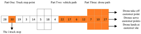
Figure 5. Schematic diagram of path coding.

A genetic algorithm increases population diversity through cross-operation to improve global search ability. In this paper, two methods of overall chromosome cross and partial chromosome cross are proposed, as shown in Figure 6 and Figure 7. Specific steps are as follows:

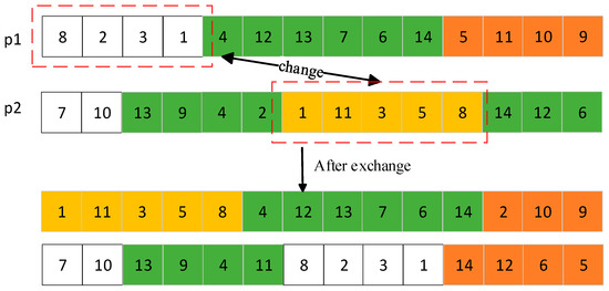
Figure 6. Global crossover operation of chromosomes.

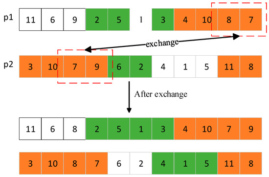
Figure 7. Chromosome partial cross operation.

Firstly, individual p1 decides whether to operate according to the crossover probability pc.

Secondly, the number of crossings is randomly determined according to the length of the two individuals.

Then, pick a random crossover. Two random numbers are generated by the overall crossover to determine the selected chromosomes a and b in individuals p1 and p2. Different genes of chromosomes a and b are stored in the gene banks Fa and Fb, respectively. At the same time, chromosomes a and b are exchanged in individuals p1 and p2 and their gene order remains unchanged. In partial crossover, gene fragments a (8,7) and b (7,9) are randomly selected from individuals p1 and p2, and different genes are stored in gene banks Fa (8) and Fb (9); two gene fragments a and b are exchanged and connected with previous chromosomes.

Finally, the chromosomes in individual p1 (except chromosome a) are compared with gene bank Fb one by one. If the genes of the chromosomes in individual p1 are duplicated with the genes in gene bank Fb, and the gene bank Fa does not contain any genes, the duplicate genes are directly deleted from individual p1. Otherwise, duplicate genes in individual p1 are successively replaced with genes in gene bank Fa, while the replaced genes are deleted in gene bank Fa. If there are still genes in Fa gene bank after the comparison of genes in individual p1, the remaining genes in Fa gene bank will be added to the last chromosome. Subsequently, perform a similar operation for individual p2.

The local searchability of the genetic algorithm is improved by mutation operation to generate new individuals. In this paper, two multiple transformation and mutation operations are proposed, namely, intra-chromosome and inter-chromosome mutation operations, as shown in Figure 8 and Figure 9. The specific steps are as follows:

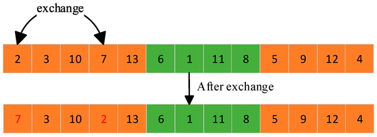
Figure 8. Intra-chromosome variation.

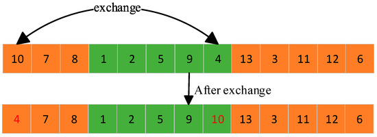
Figure 9. Inter-chromosome variation.

Step 1: Individual p chooses whether to operate according to the mutation probability pm;

Step 2: Determine the number of variations randomly according to the length of the individual;

Step 3: Select one of the two methods, intra-chromosome variation or inter-chromosome variation, at random. Intra-chromosome variation: a chromosome is randomly selected in individual p and placed on that chromosome. Two mutation points are randomly selected. Inter-chromosome variation: two chromosomes are randomly selected from individual p, the number of variations is determined according to the shortest length of chromosomes and a mutation point is selected from the two chromosomes;

Step 4: Exchange two genes;

3.3. UAV Operation Path Optimization

In the two-level path planning problem, the first-level vehicle path planning problem is solved, and the next step is to plan the second-level UAV path. The purpose of optimizing the operating path of UAV is to make the route of UAV travel path shortest and reduce the flight distance cost of UAV. Because the UAV is affected by load and power, it cannot start from the vehicle stopping point and then return to the vehicle stopping point.

The steps to optimize the operation path of UAV are as follows:

Step 1: Take the UAV directly from the docking point to a single customer point as the original distribution path;

Step 2: Calculate the distance between each customer point and the stopping point, and the distance between each customer point;

Step 3: Select a customer point as the starting point of the distribution path;

Step 4: Select the customer points around a selected customer point that are the shortest distance from the endpoint of the sub-distribution path and are not included in other sub-distribution path, then judge whether the total distance of the sub-distribution path after it is included in the sub-distribution path meets the maximum distance of UAV distribution. If so, go to Step5; otherwise, go to Step7;

Step 5: Take the customer points that are the shortest distance from the endpoint of the sub-distribution path and are not included in other sub-distribution paths as the next points of the sub-distribution path;

Step 6: Repeat Step4;

Step 7: Select a customer point that is not included in other sub-distribution paths as the starting point of the next sub-distribution path, and repeat Step3 until all customer points have been included in the sub-distribution path or optimized as the starting point of the sub-distribution path;

Step 8: Select the next customer point as the starting point of the distribution path and repeat Step2 until all customer points have been optimized as the starting point of the distribution path;

Step 9: Calculate the total distance of each distribution path and select the distribution path with the shortest distance;

Step 10: Output results.

The pseudo-code of a UAV running path optimization is shown in Algorithm 1.

Algorithm 1. UAV path optimization pseudo-code

INPUT Vehicle docking point set $V$$, \mathrm{Sample} \mathrm{set} \mathrm{of} \mathrm{customer} \mathrm{points} \left\{S_1,S_2,\cdots S_m\right\}$

$\mathrm{OUTPUT} \mathrm{Shortest} \mathrm{flight} \mathrm{path} \mathrm{of} \mathrm{UAV}\left\{x_1,x_2,\cdots x_n\right\}=\left\{\left[S_i,\cdots \right],\left[S_j,\cdots \right],\cdots \right\}$

1. $\mathrm{for} i\leftarrow 1$ to m do

2. $\mathrm{Calculate} \mathrm{the} \mathrm{distance} \mathrm{between} \mathrm{the} \mathrm{customer} \mathrm{point} \mathrm{and} \mathrm{the} \mathrm{bus} \mathrm{stopping} \mathrm{point} d_{i0}=\left|S_i-V\right|$

3. $\mathrm{Calculate} \mathrm{the} \mathrm{distance} \mathrm{between} \mathrm{this} \mathrm{customer} \mathrm{point} \mathrm{and} \mathrm{other} \mathrm{customer} \mathrm{points} dij=\left|S_i-S_j\right|$

4.  end for

5. $\mathrm{When} \mathrm{the} \mathrm{UAV} \mathrm{delivers} \mathrm{according} \mathrm{to} \mathrm{arrangement} xi=\left[S_{\alpha },S_{\beta },\cdots S_{\gamma }\right]$$, \mathrm{the} \mathrm{delivery} \mathrm{distance} \mathrm{is} d_i=d_{\alpha 0}+d_{\alpha \beta }+\cdots d_{\alpha \gamma }$

6. $\mathrm{The} \mathrm{total} \mathrm{distance} \mathrm{of} \mathrm{UAV} \mathrm{delivery} \mathrm{according} \mathrm{to} \mathrm{distribution} \mathrm{path} x_r=\left\{x_1,x_2,\cdots ,x_t\right\}$$\mathrm{is} D_r={\displaystyle \sum _{i=1}^t{d}_i}$

7. $X_0=\left\{x_1,x_2,\cdots ,x_m\right\}=\left\{\left[S_1\right],\left[S_2\right],\cdots \left[S_m\right]\right\}$

8. $D_0=2{\displaystyle \sum _{i=1}^m{d}_{i0}}$

9. $\mathrm{for} r\leftarrow 1$ to m do

10. $i\leftarrow r$

11. $x_r=X_0$

12.     repeat

13. $\eta =\arg {\min }_{j\in \left\{0,1,2\cdots m\right\}}{d}_{\omega j}$

14. $\mathrm{if} d_i-d_{\omega 0}+d_{\omega \eta }+d_{\eta 0}\le D_{\max }$ then

15. $x_i\leftarrow \left[S_{\alpha },S_{\beta },\cdots S_{\omega },S_{\eta }\right]$$// \mathrm{Let} S_{\eta }$$\mathrm{be} \mathrm{the} \mathrm{next} \mathrm{point} \mathrm{in} x_i$

16. $x_r\leftarrow x_r-\left[S_{\eta }\right]$

17. $\mathrm{else} i\leftarrow 1$

18. $\mathrm{until} i\leftarrow 1$

19. $\mathrm{Calculate} \mathrm{the} \mathrm{UAV} \mathrm{distribution} \mathrm{distance} D_r={\displaystyle {\sum }_{i=1}^t{d}_i}$$\mathrm{according} \mathrm{to} \mathrm{the} \mathrm{distribution} \mathrm{path} xr=\left\{x_1,x_2,\cdots x_t\right\}$

20. end for

21. $\lambda =\arg {\min }_{r\in \left\{0,1,2,\cdots m\right\}}{D}_r$

4. Example Verification and Analysis

4.1. K-Means ++ Clustering Algorithm Verification

In order to verify the effectiveness of the model and algorithm, the two-stage vehicle–UAV collaborative distribution algorithm designed in this chapter is compared with the single-vehicle distribution. Examples of different data scales in standard examples are used as analysis objects. The speed of the truck is set at 60 km/h and the speed of the drone is set at 80 km/h. The time for the UAV to load and take off from the truck is set to 120 s, the time for the UAV to land on the truck and change the battery is set to 120 s, the maximum flight distance of the UAV is 60 km, the maximum load of the UAV is 41 kg and the impact factor of the UAV power consumption is 0.25.

This chapter attempts to compare the improved K-means ++ clustering algorithm with the traditional K-Means clustering algorithm, in order to prove the effectiveness of the improved algorithm. However, the traditional K-means clustering algorithm does not have K value adaptability, that is to say, it cannot be solved when the K value is not selected. Therefore, this paper only studies the comparison between the vehicle UAV collaborative distribution model and the single-vehicle distribution model.

In the process of model establishment and algorithm design in this paper, it is assumed that only single-vehicle–single-UAV is used for distribution, but, in real life, multiple UAVs are often used to coordinate with each other to improve distribution efficiency and reduce distribution costs. Therefore, the concept of single-vehicle–multi-UAV distribution is introduced in this section, with no upper limit for the number of UAVs. The waiting time of the vehicle, that is, the delivery time of the drone, is reduced to the ratio of the furthest delivery distance of the drone to the flight speed of the drone. Drone takeoffs and landings are also not included in the total delivery time. The distribution time expression of single-vehicle–multiple-UAVs is shown in Equation (46):

$$T^{mCV}=\sum _{i\in V\cup S}\sum _{j\in V\cup S}\frac{x_{ij}}{V_v}+{\displaystyle \sum _{i\in S}}{\displaystyle \sum _{j\in S}}\frac{{x_{ij}}^{\max }}{V_u}$$

(46)

$T^{cv}$ represents the shortest delivery time obtained by the improved K-Means ++ clustering algorithm for single-vehicular and single-UAV cooperative distribution, and $T^{mcv}$ represents the shortest delivery time obtained by the improved K-Means ++ clustering algorithm for single-vehicular and multi-UAV cooperative distribution. $T^{GA}$ represents the shortest delivery time obtained by single vehicle distribution genetic algorithm, $T^{T\mathrm{s}}$ represents the shortest delivery time obtained by single vehicle distribution tabu search algorithm, $T^{AS}$ represents the shortest delivery time obtained by single vehicle delivery ant colony algorithm. $t_1$ is the running time of K-means++ clustering algorithm improved by vehicle–UAV cooperative distribution under each calculation example, and the running results of single-vehicle–UAV and single-vehicle–multiple UAVs can be obtained simultaneously. $t_2$ is the average running time of the three classical meta-heuristic algorithms for single-order vehicle delivery for each example. We define $GA{P}_1=(T^{op}-T^{cv})/T^{cv}\times 100\%$, that is, the percentage gap between the target value of the improved K-Means ++ clustering algorithm and the optimal value of the three classical meta-heuristic algorithms in each example; $GA{P}_2=(T^{op}-T^{mcv})/T^{mcv}\times 100\%$, which refers to the percentage gap between the target value of the improved K-Means ++ clustering algorithm and the optimal value of the three classical meta-heuristic algorithms in each example. The specific results are shown in Table 3.

Table 3. Model algorithm and validity test.

Example	Customer Point	${\mathit{T}}^{\mathit{c}\mathit{v}}\left(\mathbf{h}\right)$	${\mathit{T}}^{\mathit{m}\mathit{c}\mathit{v}}\left(\mathbf{h}\right)$	Single-Vehicle Distribution			${\mathit{t}}_1\left(\mathbf{s}\right)$	${\mathit{t}}_2\left(\mathbf{s}\right)$	$\mathit{G}\mathit{a}{\mathit{p}}_1\left(\mathit{\%}\right)$	$\mathit{G}\mathit{a}{\mathit{p}}_2\left(\mathit{\%}\right)$
				${\mathit{T}}^{\mathit{G}\mathit{A}}\left(\mathbf{h}\right)$	${\mathit{T}}^{\mathit{T}\mathit{S}}\left(\mathbf{h}\right)$	${\mathit{T}}^{\mathit{A}\mathit{S}}\left(\mathbf{h}\right)$
A-n32-k5	31	13.61	9.20	9.02	8.85	7.15	2.0	14.1	−47.5	−22.3
A-n39-k6	38	17.18	7.96	11.04	10.05	8.07	2.1	21.5	−53.0	1.4
A-n48-k7	47	19.53	8.75	13.53	11.24	8.97	2.1	29.8	−54.1	2.5
A-n55-k9	54	22.61	7.35	16.49	11.39	8.76	2.3	30.8	−61.3	19.1
A-n65-k9	64	18.29	9.30	19.60	15.26	9.86	2.5	41.8	−46.4	6.0
A-n80-k10	79	22.53	14.02	25.78	16.84	12.35	3.0	43.9	−45.2	−11.9
B-n31-k5	30	6.73	5.65	5.74	5.80	3.26	2.0	20.8	−51.6	−42.3
B-n34-k5	33	6.95	6.63	7.47	7.37	4.12	2.0	20.9	−40.7	−37.8
B-n38-k6	37	8.84	5.07	8.89	8.63	5.14	2.0	22.1	−41.8	1.3
B-n43-k6	42	12.24	4.63	8.31	7.64	5.00	2.1	25.1	−59.1	29.6
B-n45-k6	44	11.80	5.92	7.23	6.68	4.56	2.9	23.8	−61.3	−22.9
B-n51-k7	50	12.62	8.45	12.24	10.53	6.15	3.0	30.1	−51.3	−27.2
B-n67-k10	66	13.44	7.99	16.58	16.58	6.74	3.0	40.9	−49.8	−15.6
P-n16-k8	15	4.04	3.52	2.57	2.57	2.28	2.0	2.4	−43.6	−35.2
P-n20-k2	19	4.73	3.66	2.98	2.98	2.64	2.0	2.4	−44.1	−27.8
P-n23-k8	22	5.33	5.34	3.43	3.43	2.82	2.0	2.8	−47.0	−22.9
P-n45-k5	44	13.61	5.11	9.14	9.14	6.60	2.8	27.6	−51.5	23.6
P-n50-k8	49	13.62	5.36	8.51	8.51	6.34	2.8	27.9	−53.4	24.0
P-n60-k10	59	15.68	7.61	11.81	11.81	7.41	3.0	29.6	−52.7	38.3
P-n101-k4	100	21.89	3.66	21.26	21.26	10.71	3.0	57.6	−51.1	40.7

As can be seen from the above table:

(1) Under ideal conditions, that is, when the vehicle capacity is infinite, the road network is dense (the distance between customer points and customer points can be regarded as Euclidean distance) and the road congestion is good, the distribution efficiency of vehicle–UAV collaborative distribution is inferior to that of single-vehicle distribution. Especially when there is only one vehicle and one UAV to carry out the delivery task, the delivery time is 50% to 60% longer than the single-vehicle delivery. Even if a single vehicle and multiple drones deliver at the same time, for some examples, the delivery time is extended by 20–30%. Therefore, it is more reasonable to use vehicles for logistics distribution in cities with dense road networks and good road conditions;

(2) For large-scale calculation cases with more than 37 customer points, the distribution efficiency of single-vehicle–multi-UAV collaborative distribution is higher than that of single-vehicle distribution. This is because, as the number of customer points increases, the number of drones used also increases, reducing delivery time. The three large-scale examples, B-n45-k6, B-n51-k7 and B-n67-k10, have a low total. At the same time, the customer points are relatively scattered. After clustering, the number of vehicle stops increases, and the flight distance of UAV is relatively long. Therefore, the distribution time is correspondingly extended, which is longer than that of single-vehicle distribution. It can be seen that vehicle–UAV collaborative distribution is more suitable for areas with relatively concentrated customer points and clustered distribution between customer points.

4.2. Multi-Chromosome Genetic Algorithm Verification

This section verifies the superiority of the improved algorithm in terms of performance and solvability in the optimization of vehicle running path compared with the traditional genetic algorithm. The parameters involved in the multi-chromosome genetic algorithm and the traditional genetic algorithm are the same in terms of setting, and the vehicle path search process is the same. The specific parameter values are shown in Table 4.

Table 4. Parameters of genetic algorithm.

Population Number	Number of Iterations	Crossover Probability	Probability of Variation
500	2000	0.9	0.095

The proposed poly staining was performed using the standard MDVRP test case set publicly available on the International NEO website Volume genetic algorithm for testing, and the p02, p03, p12, pr01 and pr07 cases in the case set were selected. The results of the two algorithms run independently 10 times were recorded. Best refers to the best result of the algorithm run 10 times. The error calculation formula is shown in Formula (47), and the experimental results are shown in Table 5.

$$\frac{be\mathrm{s}t-known \mathrm{to} \mathrm{the} \mathrm{optimal} \mathrm{solution}}{known \mathrm{to} \mathrm{the} \mathrm{optimal} \mathrm{solution}}\times 100\%$$

(47)

Table 5. Experimental results of algorithm comparison.

Data Set	Known to the Optimal Solution	Poly Chromosome Genetic Algorithm		Traditional Genetic Algorithm
		Best	Error	Best	Error
P02	473.53	474.66	0.24%	575.61	21.56%
P03	641.19	651.82	1.75%	784.77	22.39%
P12	1318.95	1357.23	2.90%	1701.68	29.02%
Pr01	861.32	866.5	0.60%	1070.94	24.34%
Pr07	1089.56	1102.61	1.19%	1371.19	25.85%
average			1.34%		24.63%

As can be seen from Table 5, the multi-chromosome genetic algorithm proposed in this paper has a strong ability to process the data set within a certain period of time. However, with the increase in the number of customers and distribution centers in the data set, the error between the optimal solution obtained within a certain period of time and the known optimal solution becomes larger and larger. The error of the poly chromosome genetic algorithm and the known optimal solution is smaller than that of the traditional genetic algorithm. Meanwhile, the error value of the poly chromosome genetic algorithm is less than 3.5%, and the average error value is 1.75%. The error value of a traditional genetic algorithm is more than 20%, and its average error value is 24.63%. It can be concluded that the multi-chromosome genetic algorithm proposed in this paper can greatly improve the quality of solving vehicle routing problems.

5. Case Analysis

This paper uses MATLAB2019b for programming. The model is run on a Windows 10 64-bit operating system; the computer is configured with 2.6 GHz, 16 GB memory and an i7 processor. Because the actual situation is different from the ideal state, the parameters set in this chapter are slightly different from the analysis in the previous example. From the practical level, in order to comprehensively analyze the truck–drone collaborative distribution mode, this chapter not only studies the total distribution time of the two distribution modes, but also adds the calculation of distribution cost c. The distribution cost calculation formula is shown in Formula (48):

$$C=C_V+C_u+C_w+C_f$$

(48)

Among them, $C_v$ represents the vehicle driving cost, $C_u$ represents the UAV driving cost, ${\mathrm{C}}_w$ represents the vehicle waiting cost, and ${\mathrm{C}}_f$ represents the battery replacement cost for each takeoff and landing of the UAV. The basic parameters of the improved truck and UAV are shown in Table 6. UAV parameters refer to the content published by Mobs. The relationship between UAV flight distance and load is shown in Figure 10.

Table 6. Basic parameters of vehicle and UAV.

	Vehicle	UAV
Travel/flight speed (km/h)	50	80
Maximum load (kg)	Unlimited	40
The longest drive/flight distance (km)	Unlimited	40
Battery replacement time (h)	---	0.1
Influence factors of UAV power consumption	---	0.25
Driving cost (CNY/min)	1	0.5
Waiting cost (CNY/min)	0.3	---
Battery replacement cost (CNY/time)	---	1

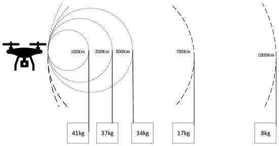
Figure 10. Relation between flight distance and load of UAV.

This chapter chooses a county (named County A) in Jiangsu Province as a case for analysis, regards the center of the county as a warehouse, selects 20 representative villages and towns around the county as customer points and each distribution point has its own different parcel demand. The location diagram of County A and each customer point is shown in Figure 11.

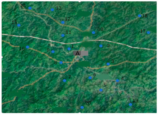
Figure 11. Location diagram of distribution center and customer point in County A, Jiangsu Province.

The demands of customer points on a certain day are shown in Table 7.

Table 7. Customer point demand.

Customer Point	Demand (kg)	Customer Point	Demand (kg)
1	9	11	7
2	2	12	11
3	5	13	39
4	8	14	3
5	4	15	10
6	4	16	5
7	29	17	9
8	38	18	23
9	17	19	8
10	4	20	12

Since the truck route is not a straight-line distance between the two places, this paper obtains the shortest road distance between the warehouse and 20 customer points and each customer point through the shortest driving route between the two places in the AutoNavi map APP, and the specific data are shown in Table 8.

Table 8. The shortest road distance between the warehouse and the customer point.

Position	Distribution Station	1	2	3	4	5	6	7	8	9	10	11	12	13	14	15	16	17	18	19	20
warehouse	---	10	24	31	48	50	30	57	32	22	29	27	34	56	63	59	54	65	67	77	58
1	10	---	30	38	55	52	73	41	18	16	28	17	29	45	57	51	47	73	74	80	64
2	24	30	---	21	41	46	37	51	40	44	18	38	42	55	75	76	65	46	47	68	57
3	31	38	21	---	20	30	22	43	42	51	38	50	59	77	89	87	74	48	57	45	52
4	48	55	41	20	---	18	26	49	55	63	55	68	78	99	95	92	86	58	72	28	44
5	50	52	46	30	18	---	18	38	46	60	59	66	78	97	92	97	80	75	94	33	28
6	30	73	37	22	26	18	---	25	31	45	48	51	63	78	88	82	62	71	78	47	32
7	57	41	51	43	49	38	25	---	19	34	57	49	61	75	82	70	49	89	92	67	35
8	32	18	40	42	55	46	31	19	---	16	48	29	43	56	64	57	36	84	86	77	50
9	22	16	44	51	63	60	45	34	16	---	42	19	34	45	49	31	24	85	87	89	68
10	29	28	18	38	55	59	48	57	44	42	---	28	29	44	60	68	61	50	45	82	78
11	27	17	38	50	68	66	51	49	29	19	28	---	14	34	42	40	37	78	72	91	88
12	34	29	42	59	78	78	63	61	43	34	29	14	---	88	34	47	32	77	69	96	98
13	56	45	57	77	99	91	78	75	56	45	44	31	18	---	21	36	46	87	78	99	91
14	63	57	75	89	98	94	88	82	64	49	60	42	34	21	---	21	50	93	95	56	98
15	59	51	76	87	95	97	82	70	57	31	68	41	40	36	21	---	52	96	76	96	92
16	54	47	65	74	86	80	62	49	36	24	61	37	32	46	40	52	---	66	93	76	79
17	65	73	46	48	58	75	71	89	84	85	50	78	77	87	93	66	95	---	20	89	95
18	67	74	47	57	72	94	78	99	86	87	45	72	69	78	95	76	93	20	---	76	93
19	77	80	68	45	28	33	47	67	77	89	85	97	60	96	98	56	96	76	89	---	45
20	58	64	67	52	44	28	32	35	50	68	78	88	99	91	98	92	79	95	93	45	---

The shortest route distance of the UAV is the linear distance between the two places. The direct linear distance data of the two places are obtained according to the linear distance measurement function of the AutoNavi map APP, as shown in Table 9.

Table 9. The distance between the distribution station and the distribution point, and the UAV route between each distribution point.

Position	Distribution Station	1	2	3	4	5	6	7	8	9	10	11	12	13	14	15	16	17	18	19	20
warehouse	---	6	14	18	28	29	17	33	19	13	17	16	20	32	37	34	31	38	39	45	34
1	6	---	18	22	32	31	43	24	11	9	17	16	20	27	34	30	28	43	44	47	38
2	14	18	---	25	25	28	22	31	24	26	11	10	17	34	45	46	39	28	28	41	40
3	18	22	13	---	11	17	13	25	24	29	22	23	25	44	51	50	42	27	32	26	30
4	28	31	25	11	---	11	16	30	34	38	34	29	48	62	64	62	52	35	44	17	27
5	29	32	28	17	11	---	11	22	27	35	35	41	46	53	60	57	47	44	55	19	16
6	17	43	22	13	16	11	---	15	18	27	29	39	37	46	52	49	37	42	42	21	19
7	33	24	31	25	30	27	15	---	12	21	35	30	25	46	50	43	30	54	62	28	21
8	19	11	24	24	34	22	18	21	---	9	24	30	19	32	37	33	21	48	49	44	29
9	13	9	26	29	38	35	27	35	9	---	25	17	18	25	27	17	13	48	49	50	38
10	17	17	11	22	34	35	29	30	25	11	---	11	8	17	37	41	37	31	27	50	48
11	16	10	23	29	41	39	30	37	17	29	17	---	10	19	25	25	22	47	43	55	53
12	20	27	25	34	48	46	37	46	25	25	18	8	---	10	19	23	18	44	39	58	56
13	32	34	34	44	62	53	46	50	32	27	27	19	10	---	12	21	27	51	46	69	66
14	37	30	45	51	64	60	52	43	37	17	37	25	19	12	---	13	25	70	65	79	67
15	34	28	46	50	62	57	39	30	33	13	41	25	23	21	13	---	35	40	46	34	62
16	31	43	39	47	52	47	47	54	21	48	37	22	18	27	25	32	---	60	59	61	45
17	38	44	28	22	35	44	42	62	48	49	21	47	44	51	70	40	60	---	12	46	58
18	39	47	28	26	44	55	46	61	49	44	27	43	39	46	65	46	59	12	---	55	64
19	45	38	41	30	17	19	28	21	44	59	50	55	58	69	79	34	61	46	55	---	27
20	34	26	40	27	27	16	19	41	29	38	48	53	56	66	67	62	45	58	64	27	---

The total delivery time of the improved truck–drone CVP-D delivery scheme and the improved former truck–drone CVP-D delivery scheme were calculated, and the results of the three schemes were compared to verify the feasibility of truck–drone collaborative delivery in real life.

In order to prevent too much error, this paper does not establish a coordinate system to visually project the position of the warehouse and the customer point in the figure, but this does not have any impact on the final result.

According to the parameter Settings in Table 7, simulation experiments were conducted on the two distribution modes respectively to obtain the total distribution time and total distribution cost, as shown in Table 10 and Table 11.

Table 10. Order of UAV visits and delivery time before improvement.

Vehicle Parking Point	Order of UAV Visits to Customer Points		Delivery Time (h)	Delivery Cost (CNY)
1	1:	1→9→11	10.92	665.2
	2:	13
	3:	14
	4:	15→16
2	1:	8
	2:	7
3	1:	5→20
	2:	3→6→4
	3:	5→19
4	1:	2→10
	2:	17→18

Table 11. The order of UAV visit and delivery time after improvement.

Vehicle Parking Point	Order of UAV Visits to Customer Points		Delivery Time (h)	Delivery Cost (CNY)
1	1:	1→11→12	9.16	534.4
	2:	13
	3:	14
	4:	15→16→9
2	1:	8
	2:	7
3	1:	20
	2:	3→4
	3:	6→5
	4:	19
4	1:	2→10
	2:	17→18

This section applies the truck–drone collaborative distribution mode to real life, selects rural areas in Jiangsu Province as the research object and calculates the real highway distance and linear distance between County A and 20 surrounding villages and towns as the distance matrix for trucks and drones to obtain the total distribution time and total distribution cost of the improved distribution mode. According to the data in the table, it can be seen that the improved truck–drone CVP-D distribution scheme is significantly optimized compared with the former one in terms of both time and cost, with a time saving of 16% and cost saving of 19%.

6. Conclusions

This paper studies the problem of route planning in the case of truck–drone cooperative distribution. Since this distribution mode is a new logistics distribution mode proposed in recent years, this paper first clarified the definition of the collocation mode of drones and trucks, that is, CVP-D. For this distribution mode, a mixed integer programming model is established, the constraints are clearly defined, and a suitable improved algorithm is designed to solve it. The effectiveness of the model and algorithm is verified by a standard calculation example. Finally, the scenarios applicable to the two distribution modes are analyzed by a real case, which has certain practical significance.

In this paper, an improved K-Means++ clustering algorithm is designed according to the characteristics of the CVP-D combination pattern, and the standard example is solved. By comparing the delivery time of single-truck and single-drone coordinated delivery, single-truck–multiple-drone coordinated delivery and single-truck delivery, it is found that the delivery time of single-truck–single-drone coordinated delivery is increased by 30–40% compared with that of single truck delivery, and the time of single-truck–multiple-drone coordinated delivery is shortened by 10% compared with that of single truck delivery in the calculation example with more concentrated customer points. In terms of solving speed, the efficiency of the improved K-Means++ clustering algorithm is much higher than that of the classical meta-heuristic algorithm. Then, the driving path of the vehicle is optimized, and a multi-chromosome genetic algorithm is designed based on the genetic algorithm. The standard example shows that the chromosome genetic algorithm proposed in this paper has a strong ability to process the data set in a certain period of time, but with an increase in the number of customers and distribution centers in the data set, the error between the obtained optimal solution and the known optimal solution in a certain period of time also increases. The errors in the multi-chromosome genetic algorithm and the known optimal solutions are smaller than those in the traditional genetic algorithm and the simulated annealing algorithm. Meanwhile, the error values in the multi-chromosome genetic algorithm are less than 3.5%, and the average error value is 1.75%.

The real data for County A in Jiangsu Province were introduced as a case study to calculate the distribution scheme before and after the algorithm improvement and their respective distribution time and distribution cost. It was found that the improved truck–drone CVP-D distribution scheme was significantly optimized in terms of both time and cost compared with the pre-improved one; the time saving was roughly 16%, and the cost savings were roughly 19%.

Due to limited time and energy, there are still many shortcomings in this paper. Although this paper has tried its best to proceed from reality and consider the limitations of realistic conditions as much as possible, the interference caused by other influencing factors in the course of UAV flight is still outside the scope of this paper. For example, the influence of wind conditions, urban no-fly zones, weather factors on UAV flight and the three-dimensional path design of UAV. We hope that, in future studies, we can take these factors into account within the model.

References

- Murray, C.C.; Chu, A. The flying sidekick traveling salesman problem: Optimization of drone-assisted parcel delivery. Transp. Res. Part C-Emerg. Technol. 2015, 54, 86–109. [Google Scholar] [CrossRef]
- Agatz, N.; Bouman, P.; Schmidt, M. Optimization Approaches for the Traveling Salesman Problem with Drone. Transp. Sci. 2018, 52, 965–981. [Google Scholar] [CrossRef]
- Ferrandez, M.; Harbison, T.; Weber, T.; Sturges, R.; Rich, R. Optimization of a truck-drone in tandem delivery network using k-means and genetic algorithm. J. Ind. Eng. Manag. 2016, 9, 374–388. [Google Scholar] [CrossRef]
- Yurek, E.E.; Ozmutlu, H.C. A decomposition-based iterative optimization algorithm for traveling salesman problem with drone. Transp. Res. Part C Emerg. Technol. 2018, 91, 249–262. [Google Scholar] [CrossRef]
- Ponza, A. Optimization of Drone-Assisted Parcel Delivery; University of Padova: Padua, Italy, 2016. [Google Scholar]
- Freitas, J.C.; Penna, P.H.V. A variable neighborhood search for flying sidekick traveling salesman problem. Int. Trans. Oper. Res. 2020, 27, 267–290. [Google Scholar] [CrossRef]
- Mbiadou Saleu, R.G.; Deroussi, L.; Feillet, D.; Grangeon, N.; Quilliot, A. An iterative two-step heuristic for the parallel drone scheduling traveling salesman problem. Networks 2018, 72, 459–474. [Google Scholar] [CrossRef]
- Bouman, N.; Agatz, N.; Schmidt, M. Dynamic programming approaches for the traveling salesman problem with drone. Networks 2018, 72, 528–542. [Google Scholar] [CrossRef]
- Carlsson, J.G.; Song, S.Y. Coordinated logistics with a truck and a drone. Manag. Sci. 2018, 64, 4052–4069. [Google Scholar] [CrossRef]
- Poikonen, S.; Golden, B.L.; Wasil, E.A. A branch-and-bound approach to the traveling salesman problem with a drone. Inf. J. Comput. 2019, 31, 335–346. [Google Scholar] [CrossRef]
- Phan, A.T.; Nguyen, T.D.; Pham, Q.D. Traveling salesman problem with multiple drones. In Optimization and Decision Science: Methodologies and Appliations, SoICT 2018 Proceedings, Ninth International Symposium on Information and Communication Technology, Danang City, Vietnam, 6–7 December 2018; Association for Computing Machinery: New York, NY, USA, 2018; pp. 46–53. [Google Scholar]
- Ha, Q.M.; Deville, Y.; Pham, Q.D.; Ha, M. On the min-cost traveling salesman problem with drone. Transp. Res. Part C Emerg. Technol. 2018, 86, 597–621. [Google Scholar] [CrossRef]
- Salama, M.; Srinivas, S. Joint optimization of customer location clustering and drone-based routing for last mile deliveries. Transp. Res. Part C Emerg. Technol. 2020, 114, 620–642. [Google Scholar] [CrossRef]
- Moshref-Javadi, M.; Hemmati, A.; Winkenbach, M. A Truck and Drones Model for Last-mile Delivery: A Mathematical Model and Heuristic Approach. Appl. Math. Model. 2019, 80, 290–318. [Google Scholar] [CrossRef]
- Moshref-Javadi, M.; Lee, S.; Winkenbach, M. Design and evaluation of a multi-trip delivery model with truck and drones. Transp. Res. Part E Logist. Transp. Rev. 2020, 136, 101–887. [Google Scholar] [CrossRef]
- Chang, Y.S.; Lee, H.J. Optimal Delivery Routing with Wider Drone-Delivery Areas along a Shorter Truck-Route. Expert Syst. Appl. 2018, 104, 307–317. [Google Scholar] [CrossRef]
- Abu-Monshar, A.; Al-Bazi, A.; Palade, V. An Agent-Based Optimization Approach for Vehicle Routing Problem with Unique Vehicle Location and Depot. Expert Syst. Appl. 2022, 192, 192–116370. [Google Scholar] [CrossRef]
- Abu-Monshar, A.; Al-Bazi, A. A multi-objective centralized agent-based optimization approach for vehicle routing problem with unique vehicles. Soft Comput. 2022, 125, 125–109187. [Google Scholar]
Disclaimer/Publisher’s Note: The statements, opinions and data contained in all publications are solely those of the individual author(s) and contributor(s) and not of MDPI and/or the editor(s). MDPI and/or the editor(s) disclaim responsibility for any injury to people or property resulting from any ideas, methods, instructions or products referred to in the content. |
© 2023 by the authors. Licensee MDPI, Basel, Switzerland. This article is an open access article distributed under the terms and conditions of the Creative Commons Attribution (CC BY) license (https://creativecommons.org/licenses/by/4.0/).