Research on Spatial-Temporal Characteristics and Affecting Factors of Agricultural Green Total Factor Productivity in Jiangxi Province

Abstract

Increasing green total factor productivity is the key to achieving green development in agriculture. This study measured the green total factor productivity of Jiangxi’s agriculture, and its regional and temporal evolution characteristics were examined. The fixed-effects model was then used to investigate the model’s fundamental components empirically. The study’s findings reveal the following: During the period under review, technical change was the primary element driving the rise in the green total factor productivity of agriculture. A rising “U”-shaped trend with notable regional variances characterizes the spatial and temporal evolution. The primary factors that affect changes in green total factor productivity in agriculture include the ease of transportation, the per capita disposable income of rural residents, the level of agricultural mechanization, the degree of urbanization, the level of financial support for agriculture, and the percentage of workers in secondary industries, with the impact effect values of 0.581, 0.647, −0.126, −0.729, −0.326, and −0.559, respectively. As a result, it is suggested that in order to substantially increase agricultural green total factor productivity, agricultural green technological support should be strengthened, more fully developed, and promoted in a multi-pronged approach.

1. Introduction

Agriculture is the cornerstone of national economic development, and the green development of agriculture is a primary focus during the sustainable development of a rural economy and society [1]. The breadth and depth of agricultural exchanges between nations are at an all-time high in the modern world, where economic globalization and world integration are progressing at an unheard-of rate. However, the rapid development of agriculture still needs to improve, such as environmental pollution as a cost. According to some studies, the agriculture industry is responsible for 13% of the world’s carbon emissions [2]. Driven by the concept of sustainable development, green development has become a common choice for agricultural development and modernization worldwide [3]. Among them, China, a predominantly agricultural nation, struggles harder with the transition to green development while significantly contributing to global food security [4]. The Intergovernmental Panel on Climate Change (IPCC) of the United Nations emphasizes the complicated causal link between agricultural productivity and climate, and has stated that improper land use and management practices may increase global warming, eventually leading to a vicious cycle [5]. Additionally, 4 of the 17 Sustainable Development Goals (SDGs) of the United Nations are related to agriculture, fully illustrating the significance of greening agriculture and the necessity of promoting the transformation and upgrading of production methods, in order to ensure that agricultural production meets the 2030 Sustainable Development Goals and adapts to future development changes [6]. Agricultural Green Total Factor Productivity (AGTFP) incorporates environmental pollution into the measurement framework while using all input factors to obtain output in the agricultural production process, which not only assesses the level of agricultural economic development but also emphasizes the necessity of resource utilization and environmental protection, and is a crucial yardstick for assessing the extent of green agricultural development [7]. It is a modification of the conventional total factor productivity (TFP) concept of economic prioritization. What causes the increase in green total factor productivity in agriculture? What are its spatial and temporal qualities? What are the driving forces? The super-efficient EBM-GML model, ArcGIS 10.2 trend analysis software, and the fixed-effects model will each be used in this study to address the abovementioned problems and provide theoretical and practical references for enhancing AGTFP and examining the direction of green agricultural development.

The relationship between economic growth and resources, and environmental restrictions, has become a hotly debated subject. The three primary areas of the current discussions on green total factor productivity in agriculture are as follows. The first concerns the scope of study. There are few studies that have been undertaken on medium and microscopic scales, such as in municipalities, counties, and towns. The research primarily focuses on macro scales, such as nations, provinces, or economic areas, where data are more readily available [8]. Nevertheless, compared to the central and western parts of China, the AGTFP is often higher in the country’s more economically advanced eastern regions [9,10,11,12]. The measurement methods are the second area of concern. The two main techniques are stochastic frontier analysis (SFA) and data envelopment analysis (DEA), with DEA being more commonly used by academics. When calculating the green total factor productivity, the Malmquist index and DEA method are typically used as the base model and index. DEA has evolved to yield a variety of models; among them, the Epsilon-based Measure (EBM) model [13] is a good choice for measuring agricultural green total factor productivity because it not only satisfies the unexpected output but also resolves the issue whereby both inputs and outputs have radial and non-radial characteristics. The EBM model and the Global Malmquist–Luenberger (GML) index [14] are utilized to resolve the linear programming issue and the potential lack of workable alternatives to measure AGTFP more scientifically [15]. The influencing variables comprise the third issue. Is technological change (TC) or technical efficiency change (EC) the endogenous driver of AGTFP? The secret to AGTFP development lies herein. According to the majority of academics, technological change, not technical efficiency, is what drives increases in AGTFP. Hence, addressing the inefficiency of resource variables can significantly boost the AGTFP [16,17,18,19]. Few academics think that technical effectiveness is a significant motivation that can significantly boost AGTFP growth through improved technological innovation [20]. Some academics also contend that the “dynamic double drive” of technological change and technical efficacy is what is responsible for the expansion [21,22]. Furthermore, exogenous factors such as agricultural technology input [23], digital agriculture development [3], human capital structure optimization [24], environmental governance [12], economic growth pressure [25], agricultural fiscal expenditure [2], and the urban–rural income gap [26] all have varying degrees of effect on AGTFP changes.

In conclusion, there are many studies on AGTFP. However, some gaps still exist. Firstly, there needs to be more research undertaken on the municipal and county scales, with the majority of extant studies concentrating on the national, regional, or economic scales. Narrowing the study area and enhancing data precision is unavoidable due to the current state of substantial regional variation in AGTFP. Second, the majority of research measures currently in use still employ single radial (DEA) or single non-radial (SBM) models; however, the mixed distance function (EBM) model can successfully address the issue of both radial and non-radial input–output. Finally, there is an ongoing debate over the factors that cause AGTFP growth, and more research must be performed on these factors. In the southeast of China, Jiangxi Province is on the south bank of the middle and lower reaches of the Yangtze River. It is home to Poyang Lake, the largest freshwater lake in China, and is rich in water resources. With clear seasonal patterns and fertile soil, Jiangxi Province is dubbed “the land of fish and rice”. As the third largest producer of grain in China as of 2022, Jiangxi Province is one of the country’s major rice-producing regions. In addition, Jiangxi Province’s forest area in 2022 was 155 million mu, and its forest coverage rate was 63.35%, ranking it second in the nation. Furthermore, the national forest manager system assessment ranked it first in the nation, and this region has served as one of the first demonstration areas of national ecological civilization construction. Jiangxi Province, one of China’s “greenest” provinces, exemplifies China’s distinctive agriculture, and is a model of sustainable agricultural development. While Jiangxi Province has made a significant contribution to China’s food security, it also inevitably increases the use of chemical products such as pesticides and fertilizers, which increases the challenge to Jiangxi Province’s green agricultural development and serves as a helpful model for other less effective provinces to encourage their green agricultural development [27]. As a result, researching the green total factor productivity of agriculture in Jiangxi Province, examining its characteristics in terms of spatial and temporal evolution, and investigating its growth dynamics are beneficial in terms of addressing the shortcomings of green development, fostering agricultural transformation and upgrading, and enhancing AGTFP in other parts of China in a value-driven manner.

2. Research Methodology and Data Sources

2.1. Research Methodology

2.1.1. Super-Efficiency EBM Model

The EBM model combines radial and non-radial models, allowing for various distances to be defined for each input and output [13]. In order to measure AGTFP, it is necessary to extend the EMB model to a super-efficient EBM model that includes non-desired outputs, non-direction, and variable returns due to the complex relationships among resource factor inputs, economic outputs, and environmental outputs in the agricultural production process. These relationships include both desired and non-desired outputs and radial and non-radial relationships, given the complex relationships among resource factor inputs, economic outputs, and environmental outputs in the agricultural production process. The expansion model is as follows:

$$\begin{gathered} {\gamma }^{*}=\underset{\theta ,\lambda ,s^{-}}{\min }\frac{\theta -{\epsilon }_x{{\displaystyle \sum }}_{i=1}^m\frac{{\omega }_i^{-}{s}_i^{-}}{x_{io}}}{\phi +{\epsilon }_y{{\displaystyle \sum }}_{r=1}^s\frac{{\omega }_r^{+}{s}_r^{+}}{y_{ro}}+{\epsilon }_h{{\displaystyle \sum }}_{p=1}^q\frac{{\omega }_p^{h-}{s}_p^{h-}}{h_{po}}} \\ s.t.\{\begin{array}{c}\theta x_{io}-{\displaystyle \sum }_{j=1}^n{\lambda }_j{x}_{ij}-s_i^{-}=0,i=1,\dots ,m\\ \phi y_{ro}-{\displaystyle \sum }_{j=1}^n{\lambda }_j{y}_{rj}-s_r^{+}=0,r=1,\dots ,s\\ \phi h_{po}-{\displaystyle \sum }_{j=1}^n{\lambda }_j{y}_{pj}-s_p^{h-}=0,p=1,\dots ,q\\ s_i^{-}\ge 0,s_r^{+}\ge 0,s_p^{h-}\ge 0\\ {\lambda }_j\ge 0\end{array} \end{gathered}$$

(1)

In Equation (1) above, the decision-making unit (DMU) technique is effective when ${\gamma }^{*}$ = 1, which is the size of the ideal efficiency as determined by the super-efficient EBM model; $\mathsf{\theta }$ represents the efficiency value in the radial condition, $\mathsf{\lambda }$ represents the relative weights of the input factors; ${\mathrm{s}}_{\mathrm{i}}^{-}$ represents the amount of slack in the input factors of type i under the non-radial condition; ${\mathsf{\epsilon }}_{\mathrm{x}}$ is the core parameter satisfying $1\leqq {\mathsf{\epsilon }}_{\mathrm{x}}\leqq 1$, including the radial variation proportion and the non-radial relaxation vector; ${\mathrm{x}}_{\mathrm{io}}$ and ${\mathrm{y}}_{\mathrm{ro}}$ stand for the oth decision unit’s input–output vector, while ${\mathrm{h}}_{\mathrm{po}}$ stands for the pth decision unit’s undesired output. If the value of ${\mathrm{s}}_{\mathrm{r}}^{+}$ or ${\mathrm{s}}_{\mathrm{p}}^{\mathrm{h}-}$ is greater than 0, the actual inputs and outputs will be below the production frontier boundary level, and the production efficiency will need to be increased. For the rth desired output and the pth undesirable output, respectively, the slack vectors are denoted by ${\mathrm{s}}_{\mathrm{r}}^{+}$ and ${\mathrm{s}}_{\mathrm{p}}^{\mathrm{h}-}$. If the value is higher than 0, the production efficiency needs to be increased, because the inputs and outputs are below the production frontier border level. We here employ the MaxDEA ULTRA 9 software to give weights to the data, which can reflect the relevance of each input element and output more objectively, and thus avoid subjectivity in weight-setting.

2.1.2. Global Malmquist–Luenberger (GML) Index

The GML index, which reflects the stage of change in production efficiency, was utilized to better depict the dynamics of AGTFP. The GML index creates the production frontier surface using all DMU examination periods as benchmarks, or, more specifically, by enclosing all current period benchmarks into a single global production possibility set, acting as a standard reference set for all periods; this effectively overcomes the circular cumulative nature of linear programming and its non-solvability, and permits technical regression [28]. The precise formula is as follows:

$$GM{L}_t^{t+1}(x^t,y^t,b^t,x^{t+1},y^{t+1},b^{t+1})=\frac{1+D_G^T\left(x^t,y^t,b^t\right)}{1+D_G^T\left(x^{t+1},y^{t+1},b^{t+1}\right)}$$

(2)

The ratio of the current period’s AGTFP to that of the following period is reflected in the GML. The efficiency increases when the ${\mathrm{GML}}_{\mathrm{t}}^{\mathrm{t}+1}$ is more than 1, but the efficiency decreases when the ${\mathrm{GML}}_{\mathrm{t}}^{\mathrm{t}+1}$ is less than 1. The GML index can be further divided into technical change (TC) and technical efficiency change (EC), as follows:

$$\begin{gathered} GM{L}_t^{t+1}(x^t,y^t,b^t,x^{t+1},y^{t+1},b^{t+1})=\frac{1+D_G^T\left(x^t,y^t,b^t\right)}{1+D_G^T\left(x^{t+1},y^{t+1},b^{t+1}\right)} \\ =\frac{1+D_C^t\left(x^t,y^t,b^t\right)}{1+D_C^{t+1}\left(x^{t+1},y^{t+1},b^{t+1}\right)}\ast \left[\frac{\left(1+D_G^T\left(x^t,y^t,b^t\right)\right)/\left(1+D_C^t\left(x^t,y^t,b^t\right)\right)}{\left(1+D_G^T\left(x^{t+1},y^{t+1},b^{t+1}\right)\right)/\left(1+D_C^{t+1}\left(x^{t+1},y^{t+1},b^{t+1}\right)\right)}\right] \\ =\frac{T{E}^{t+1}}{T{E}^t}\ast \frac{P{G}_{t+1}^{t,t+1}}{P{G}_t^{t,t+1}}=E{C}^{t,t+1}\ast T{C}^{t,t+1} \end{gathered}$$

(3)

Per Zofio’s (2007) [29] methodology for the breakdown of the ML index, TC is further divided into pure technical change (PTC) and scale technical changes (STC). In contrast, EC is further divided into pure technical efficiency change (PEC) and scale efficiency change (SEC), as shown in Equation (4):

$${\mathrm{GML}}_{\mathrm{t}}^{\mathrm{t}+1}=\mathrm{EC}\ast \mathrm{TC}=\left(\mathrm{PEC}\ast \mathrm{SEC}\right)\ast \left(\mathrm{PTC}\ast \mathrm{STC}\right)$$

(4)

2.1.3. Entropy Value Method

The entropy technique is popular across many areas because it calculates index weights based on the degree of variation in the index values, rather than the bias introduced by subjective assignment [30]. Since the sources of agricultural surface pollution vary, this study uses the entropy value method to standardize each index of surface source pollution when measuring agricultural surface source pollution. Then, it integrates them into one comprehensive index, avoiding the measurement bias brought on by the scale’s inconsistency. The entropy approach is modified by including a time variable because this study uses panel data.

The first step is to set the metrics. ${\mathrm{X}}_{\mathsf{\theta }\mathrm{i}\mathrm{j}}$ denotes the value of the jth indicator for municipality i in year $\mathsf{\theta }$.

The second step is to standardize the processing approach. The extreme value method is used in this study to normalize this dimensionless step, which produces a value between 0 and 1.

The following standardizes positive indicators:

$${\mathrm{X}}_{\mathsf{\theta }\mathrm{i}\mathrm{j}}=\frac{{\mathrm{X}}_{\mathsf{\theta }\mathrm{i}\mathrm{j}}-{\mathrm{X}}_{\min }}{{\mathrm{X}}_{\max }-{\mathrm{X}}_{\min }}$$

(5)

The following standardizes negative indicators:

$${\mathrm{X}}_{\mathsf{\theta }\mathrm{i}\mathrm{j}}=\frac{{\mathrm{X}}_{\max }-{\mathrm{X}}_{\mathsf{\theta }\mathrm{i}\mathrm{j}}}{{\mathrm{X}}_{\max }-{\mathrm{X}}_{\min }}$$

(6)

The third step is to determine the weights, by:

$${\mathrm{Y}}_{\mathsf{\theta }\mathrm{i}\mathrm{j}}=\frac{{\mathrm{X}}_{\mathsf{\theta }\mathrm{i}\mathrm{j}}}{{{\displaystyle \sum }}_{\mathsf{\theta }}{{\displaystyle \sum }}_{\mathrm{i}}{\mathrm{X}}_{\mathsf{\theta }\mathrm{i}\mathrm{j}}}$$

(7)

The jth indicator’s entropy value is determined in the fourth stage.

$${\mathrm{S}}_{\mathrm{j}}=-\mathrm{r}{{\displaystyle \sum }}_{\mathsf{\theta }}{{\displaystyle \sum }}_{\mathrm{i}}{\mathrm{Y}}_{\mathrm{ij}}\ln \left({\mathrm{Y}}_{\mathsf{\theta }\mathrm{i}\mathrm{j}}\right),\mathrm{r}=\ln \left(\mathrm{kn}\right)$$

(8)

The jth indicator’s coefficient of variation is calculated in the fifth stage.

$${\mathrm{G}}_{\mathrm{j}}=1-{\mathrm{S}}_{\mathrm{j}}$$

(9)

Each of the indicators’ weights are calculated in the sixth stage.

$${\mathrm{W}}_{\mathrm{j}}=\frac{{\mathrm{G}}_{\mathrm{j}}}{{{\displaystyle \sum }}_{\mathrm{j}}{\mathrm{G}}_{\mathrm{j}}}$$

(10)

The composite score of factor inputs is determined in the seventh stage. There are typically two methods for computing the composite index. The first is multiplying the weights by the index’s standardized value (${\mathrm{X}}_{\mathsf{\theta }\mathrm{i}\mathrm{j}})$ to add them up; the second is multiplying them by the index’s standardized weight index (${\mathrm{Y}}_{\mathsf{\theta }\mathrm{i}\mathrm{j}})$ to do so. The first approach is utilized in this study.

$${\mathrm{H}}_{\mathsf{\theta }\mathrm{i}}={{\displaystyle \sum }}_{\mathrm{j}}\left({\mathrm{W}}_{\mathrm{j}}{\mathrm{X}}_{\mathsf{\theta }\mathrm{i}\mathrm{j}}\right)$$

(11)

2.2. Indicator Selection

A single standard for AGTFP measurement indicators has yet to be established. Most researchers agree that the main indicators of inputs include labor, land, fertilizer, pesticides, agricultural irrigation and agricultural film [3,31,32,33], and some scholars also include draught animals [34], capital [35], and agricultural electricity [36]. As environmental restrictions have become more severe, scientists have begun to include agricultural carbon emissions and surface source pollution to the measurement index system as undesirable outputs [6,15,37,38]. The following table describes this study’s green total factor productivity index system for agriculture (

Table 1. Measuring indicators of AGTFP.

Type of Variables		Variables and Descriptions	Unit
Input Indicators	Labor input	Primary industry employment × (total agricultural output value/total output value of forestry, animal husbandry, and fisheries)	10 thousand people
	Land input	Total area of crops sown	Hectares
	Capital input	Amount of converted agricultural chemical fertilizer applied	Ton
		Pesticide usage	Ton
		Agricultural film usage	Ton
		Total power of agricultural machinery	10 Kw
		Year-end headcount of large livestock	1 head
		Primary sector investment in fixed assets × (total agricultural output value/total output value of forestry, animal husbandry, and fisheries)	CNY 10 thousand
	Energy input	Agricultural electricity consumption	Kw·h
	Water input	Effective irrigated area	Hectares
Output Indicators	Desirable output	Total agricultural output	CNY 10 thousand
	Undesirable output	Agricultural carbon emissions	Ton
		Agricultural surface source pollution composite index	——

).

2.2.1. Input Indicators

Based on prior research and the current state of agricultural production in Jiangxi Province, five different input indicators, totaling ten measurement indicators, were chosen for this study to reflect the thoroughness and scientific nature of the indicator selection as effectively as possible. Narrowly specified agricultural workers are what define labor inputs. This indicator is calculated by multiplying the ratio of the production value of total agricultural, forestry, animal husbandry, and fishing by the total number of persons, since the statistics yearbook only contains the total number of people engaged in the primary industry. Land inputs are defined by the total area of crops sown. Fertilizer is distinguished by the amount of converted agricultural chemical fertilizer applied. The amount of agricultural chemical fertilizer used during application can be split into different types of fertilizer; the discounted amount is more uniform when compared to the amount of fertilizer applied, and the majority of studies utilize this kind. Agricultural machinery, a manifestation of agricultural modernization, has an overall power that is generally accepted. However, some scholars also use agricultural diesel fuel to characterize agricultural machinery. Considering the availability and completeness of data, this indicator is chosen to characterize the overall power of agricultural machinery. Pesticides can help avert disasters brought on by pests and diseases, but they are also the main cause of pollution and carbon emissions; this indicator was chosen to represent the level of pesticide use. Agricultural film is one of the critical components in the development of agriculture, and also contributes significantly to surface pollution and carbon emissions; the quantity of agricultural plastic film utilized defines this indication. For draft animals, the quantity of huge livestock heads at the year’s end serves as the defining characteristic. Under the funding indicator, increasing agricultural productivity starts with investments in infrastructure, including buildings, machinery, and transportation, and this statistic is calculated by multiplying the amount of fixed asset investment in the primary sector by the ratio of total agricultural output value to total agricultural, forestry, animal husbandry, and fishing output value. It is impossible to overlook agricultural water as a natural resource when producing food, and agricultural water supplies have historically had low per capita occupancy rates and low rates of usage. This indicator is characterized by the effective irrigated area. Electricity is the primary energy source used in agricultural production. At a time when energy security is prioritized, it is essential to reduce unnecessary energy consumption, and using various energy sources during agricultural production will result in significant carbon emissions; this indicator is characterized by agricultural electricity consumption.

2.2.2. Output Indicators

Desirable and undesirable outputs are included in the output indicators. The first indicator of desired output is gross agricultural output, which is deflated using 2006 as the base year to better reflect the trend in price levels. Second, the most broadly defined sources of agricultural carbon emissions include the following: carbon emissions from the production and use of contemporary production materials, such as fertilizers, pesticides, and agricultural films; carbon emissions from the direct or indirect consumption of fossil fuels by agricultural machinery; organic carbon loss caused by the destruction of soil organic carbon pools by agricultural tillage; greenhouse gas emissions caused directly or indirectly by energy consumption [31]. Pesticides, agricultural films, fertilizers, total agricultural machinery power, agricultural irrigation, and agricultural tillage are the six indicators we have chosen to measure agricultural carbon emissions. Agriculture’s overall carbon emissions are calculated via $\mathrm{E} = \sum {\mathrm{E}}_{\mathrm{i}} =\sum {\mathrm{T}}_{\mathrm{i}}{\ast \mathsf{\delta }}_{\mathrm{i}}$, where $\mathrm{E}$ stands for total agricultural carbon emissions, ${\mathrm{E}}_{\mathrm{i}}$ is each carbon source’s emission, ${\mathrm{T}}_{\mathrm{i}}$ is each source’s use, and ${\mathsf{\delta }}_{\mathrm{i}}$ is each source’s carbon emission coefficient. The respective carbon emission coefficients are fertilizer, 0.8956 kg/kg; pesticide, 4.9341 kg/kg; agricultural films, 5.18 kg/kg; tillage, 3.126 kg/hm²; and agricultural irrigation, 19.8575 kg/hm². Carbon emitted from the operation of agricultural machinery can be calculated using the following formula: ${\mathrm{E}}_{\mathrm{m}}={\mathrm{A}}_{\mathrm{m}}\ast \mathrm{B}+{\mathrm{W}}_{\mathrm{m}}\ast \mathrm{C}$, where ${\mathrm{A}}_{\mathrm{m}}$ is the total area of crops sown, ${\mathrm{W}}_{\mathrm{m}}$ is the total power of agricultural machinery, and $\mathrm{B}$ and $\mathrm{C}$ are conversion coefficients (B = 16.47 kg/hm², C = 0.18 kg/kW). Fertilizers and pesticides have been classified by the U.S. Oak Ridge National Laboratory (ORNL), the agricultural film reference of the Nanjing Agricultural University Institute of Resource, the Ecosystem and Environment of Agriculture (IREEA), the agricultural irrigation reference set out by Wang et al. [39], and the agricultural machinery reference established by Duan et al. [40]. Finally, agricultural surface source pollution is primarily caused by the underuse of modern agricultural productivity tools, such as chemical fertilizers, pesticides, and agricultural films. Accordingly, the amount of fertilizer (N and P) lost, agricultural film residues, and leftover pesticides were chosen in this study to quantify agricultural surface source pollution. The method of estimation involved the “First National Pollution Source Census Agricultural Surface Source Pollution Coefficient Manual” and Lai et al.’ s (2004) [41] inventory.

2.3. Data Source

Panel data from Jiangxi Province’s 11 prefecture-level cities from 2006 to 2021 were chosen for this study. The “Statistical Yearbook of Jiangxi Province,” the “Statistical Yearbook of China Urban and Rural Construction,” the “Statistical Yearbook of China Rural,” statistical bulletins on the national economic and social development of each district city, the EPS data platform, and statistical yearbooks of each prefecture-level city were the primary sources of data. Using Wang et al.’s [42] approach, the prior year’s growth was multiplied by the previous year’s value to compensate for aberrant or missing values.

3. Results Analysis and Discussion

3.1. Analysis of the Spatial and Temporal Properties of AGTFP

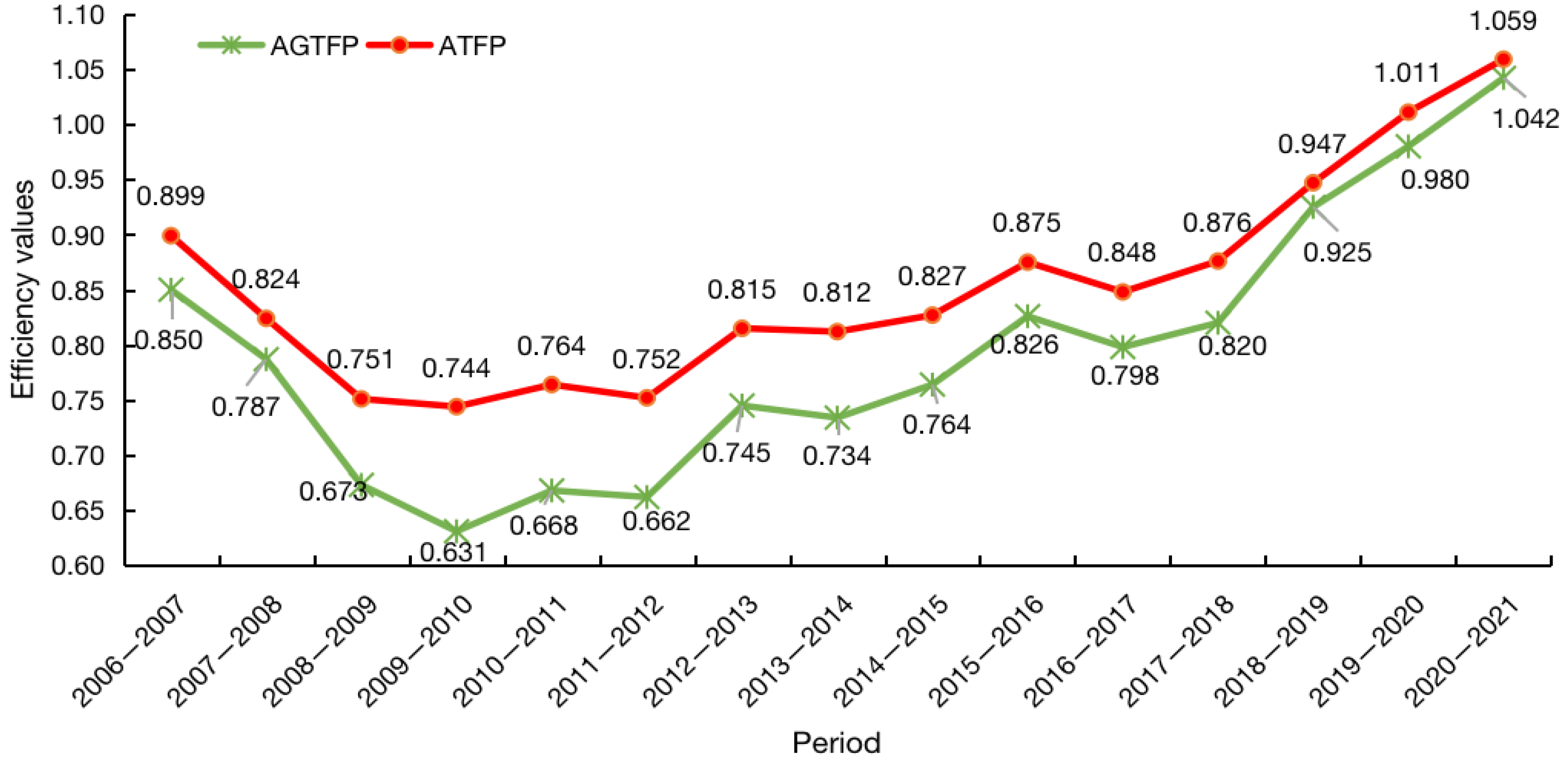
3.1.1. Comparison of AGTFP and ATFP

Agricultural total factor productivity (ATFP) without considering undesirable outputs, and agricultural green total factor productivity (AGTFP) considering carbon emissions and surface source pollution, were measured separately using the super-efficiency EBM model (Figure 1). The results show that the trends in AGTFP and ATFP were broadly similar, but AGTFP’s value was found to be much lower when it incorporated the undesirable output. Therefore, considering the effects of undesirable output when calculating agricultural production efficiency will make the results more accurate and applicable.

Overall, the trend of Jiangxi Province’s AGTFP exhibits a “U”-shaped curve, which indicates a decrease followed by an increase. The drop in food prices from 2006 to 2009 and the ongoing increases in the prices of agricultural production inputs and rural consumer goods directly impacted farmers’ returns, and ultimately resulted in less AGTFP [31]. In addition, Jiangxi Province was affected by natural disasters in 2008, including the nationwide mega-flood and uncommonly low temperatures, rain, and snow—which had a disastrous effect on agricultural productivity and may have also impaired AGTFP. However, the government quickly passed several measures that benefited the agricultural industry. Fiscal spending remained skewed in favor of agriculture, and the steps towards green development in agriculture were successful, as a result of which the AGTFP showed a general upward trend. Specifically, the average annual AGTFP values of Jiangxi Province from 2006–2010 to 2016–2020 were 0.735 and 0.870, respectively, with a growth rate of 18.37%; this demonstrates that while Jiangxi Province’s AGTFP has made some progress, there is still a gap between that situation and the current pace of agricultural development, and environmental pollution and resource utilization issues still need to be addressed.

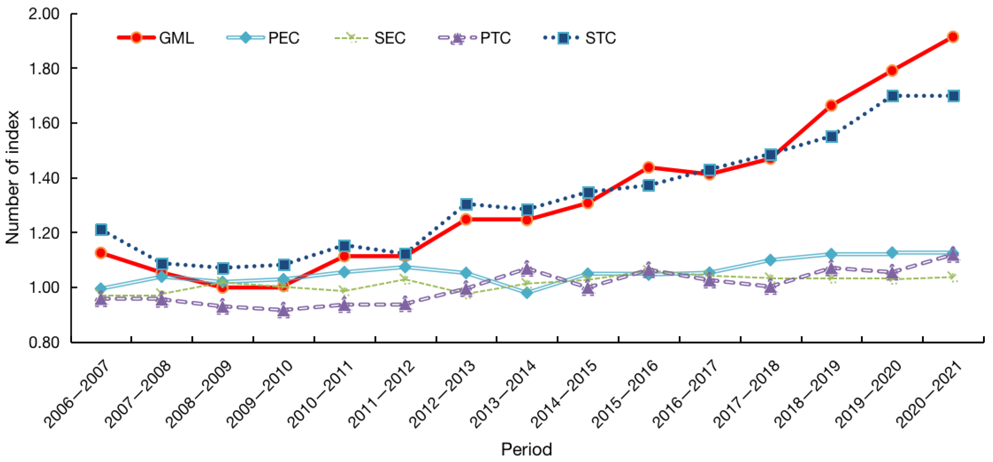
3.1.2. Characteristics of the AGTFP Time Series

The GML index can be further deconstructed to determine the AGTFP growth source (

Table 2. GML and the decomposition index.

Period	GML	EC	TC	PEC	SEC	PTC	STC
2006–2007	1.125	0.968	1.159	0.994	0.972	0.958	1.210
2007–2008	0.936	1.043	0.896	1.044	1.003	0.998	0.898
2008–2009	0.948	1.008	0.932	0.982	1.043	0.973	0.985
2009–2010	1.006	0.990	1.006	1.009	0.984	0.986	1.010
2010–2011	1.108	1.005	1.094	1.025	0.985	1.022	1.066
2011–2012	1.000	1.047	0.962	1.017	1.043	1.003	0.973
2012–2013	1.121	0.933	1.235	0.980	0.949	1.059	1.162
2013–2014	0.998	0.960	1.050	0.931	1.038	1.074	0.985
2014–2015	1.050	1.086	0.979	1.071	1.013	0.934	1.049
2015–2016	1.099	1.031	1.084	0.997	1.033	1.065	1.018
2016–2017	0.983	0.994	1.001	1.007	0.983	0.964	1.043
2017–2018	1.040	1.032	1.011	1.044	0.992	0.977	1.039
2018–2019	1.132	1.018	1.112	1.020	1.000	1.068	1.044
2019–2020	1.076	1.000	1.077	1.005	0.996	0.985	1.095
2020–2021	1.069	1.006	1.062	0.998	1.008	1.061	1.001
2006–2021	1.046	1.008	1.044	1.008	1.003	1.009	1.039

). Overall, the GML index in Jiangxi Province averaged 1.046 during the study period, which caused the AGTFP to increase. Decomposing the GML index using Equation (3) yields TC and EC indices, which have mean values of 1.044 and 1.008, respectively. This demonstrates that TC and EC contribute to the growth of AGTFP, although TC is the primary power source. Jiangxi Province has recently increased its investment in agricultural green production technology research and development, introduced high-quality and cutting-edge machinery, and strengthened its capacity to support science and technology, leading to clear results in terms of agricultural green development.

Specifically, throughout the period in question, Jiangxi Province’s GML index, TC index, and EC index all exhibit an oscillating tendency of alternating up and down. The GML and TC indices increased from 2006 to 2007, but the EC index decreased, indicating that technological change has enhanced the efficient use of resources, causing AGTFP to increase. The EC index had a value greater than 1 between 2007 and 2009. However, the AGTFP index and TC index were both below 1—as a result of the bias of technological change toward elements such as capital, labor, and natural resources—while the environment’s restricting influence was ignored, as a result of which non-green technologies developed quickly, which reduced the AGTFP. The GML index was more than 1 from 2009 to 2021, except for 2013–2014 and 2016–2017, and the TC and EC indices were also noticeably higher; technological change clearly drives AGTFP.

The GML index can be decomposed into four parts using Equation (4): SEC, STC, PTC, and PEC (Table 2). The annual average values of the decomposed indices’ PEC, SEC, PTC, and STC indices are 1.008, 1.003, 1.009, and 1.039. To more effectively visualize the development of each decomposition index and investigate the driving forces behind AGTFP growth, referring to the method of Li et al. [43], each index can be viewed as a cumulative change index, with a base year of 2006. Each index is the sum of the indices from the base year to the reporting year (Figure 2). Comparing the evolutionary tendencies of GML and STC, we found that they were very similar; this shows that the expansion of AGTFP in Jiangxi Province over the period is highly dependent on technical change (TC) and is “single-core driven” by scale technical change (STC). Green technology’s scaling up has modernized agriculture and altered the crude production paradigm, which has fueled AGTFP growth.

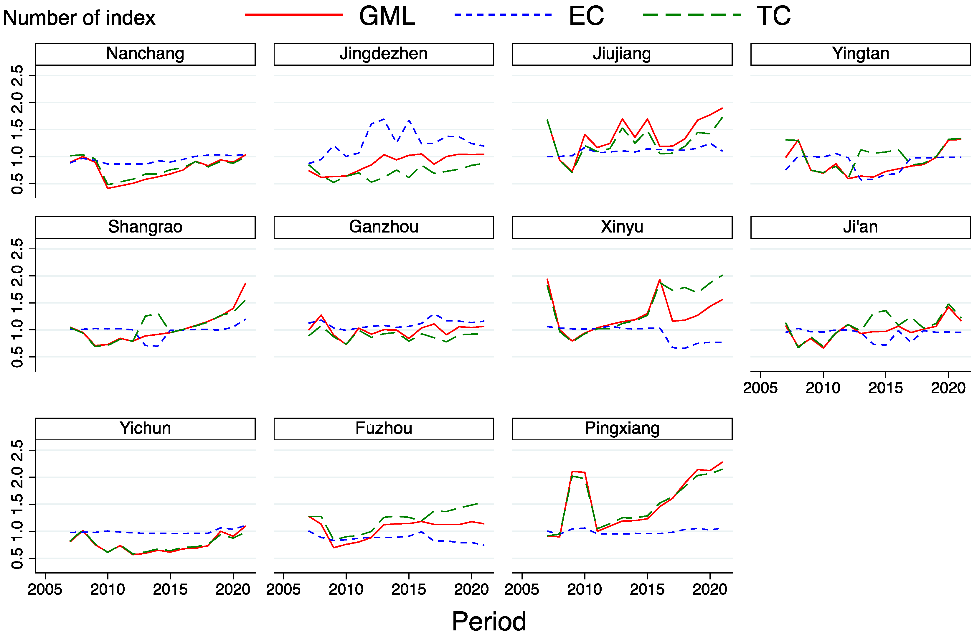
3.1.3. Characterization of the AGTFP Spatial

Spatial characterization of natural areas. Jiangxi Province can be divided into three main areas according to its geographical features: the South (Ganzhou), the Center (Fuzhou, Ji’an, Pingxiang, Yichun, and Xinyu), and the North (Nanchang, Jiujiang, Jingdezhen, Shangrao, and Yingtan) [44]. From 2006 to 2021, Jiangxi Province’s annual average AGTFP index measurement yielded the following findings (

Table 3. Natural area AGTFP index measurement results.

Period	North	Center	South
2006–2007	1.070	1.206	0.996
2007–2008	0.950	0.854	1.279
2008–2009	0.800	1.145	0.709
2009–2010	1.078	0.974	0.806
2010–2011	1.103	1.051	1.419
2011–2012	0.985	1.037	0.890
2012–2013	1.188	1.059	1.091
2013–2014	0.958	1.039	0.995
2014–2015	1.126	1.015	0.843
2015–2016	0.992	1.180	1.231
2016–2017	1.036	0.912	1.070
2017–2018	1.058	1.067	0.821
2018–2019	1.135	1.124	1.161
2019–2020	1.089	1.082	0.987
2020–2021	1.115	1.032	1.022

). The northern, central, and southern regions’ yearly average AGTFP indices all grew, with values of 1.045, 1.052, and 1.021, respectively. Among these, the average annual AGTFP of the northern area has been comparable to the province’s average annual AGTFP. The central region’s average yearly growth rate has exhibited the most pronounced tendency, and is higher than the province average, demonstrating that compared to other regions, the central region has better resource allocation and more environmentally friendly manufacturing methods, strengthening the momentum of AGTFP growth. The lowest average yearly growth rate has been seen in the South. However, in 2010–2011, the southern region’s average annual AGTFP reached 1.419, which is much higher than the province average. During this time, the southern region may have taken advantage of its abundant natural resources, such as its vast land, thus contributing to a significant increase in AGTFP. However, at the same time, it was also under pressure to optimize and improve the structure and production conditions of the agricultural industry, which ultimately resulted in a slow increase in the average annual growth rate of AGTFP in the southern region.

Spatial characterization of administrative areas. The GML, TC, and EC indices were similarly processed as cumulative change indices, using 2006 as the base period to more intuitively depict the trend of AGTFP progression in each region (Figure 3). Overall, all regions’ technological efficacy has been increasing slowly, but there are apparent regional variances in technical change, showing that this relationship differs significantly from the “dual-core drive” model. The AGTFP of each city specifically showed a declining or fluctuating trend from 2006 to 2009. From 2009 to 2021, Pingxiang, Jiujiang, Xinyu, Yingtan, and Shangrao all showed a more apparent upward trend, whereas Nanchang, Jingdezhen, Ganzhou, Ji’an, Yichun, and Fuzhou showed a less obvious upward trend, or their growth rates were still lower. Pingxiang City has shown the most extraordinary cumulative change index of them all (2.282). This is because Pingxiang City has recently undertaken the coordinated development of environmental protection and economical construction, giving full play to its advantages in terms of resources and location. Furthermore, its total energy consumption and “double control” target assessment ranked first in the province, and its agricultural green development momentum is strong.

3.1.4. Characterization of the AGTFP Spatial and Temporal Features

With the help of ArcGIS 10.2 software, trends in spatial patterns were analyzed by plotting the annual average AGTFP by region from 2006 to 2011, 2011 to 2016, and 2016 to 2021 [45]. Low-, comparatively low-, medium-, relatively high-, and high-efficiency areas are indicated by AGTFP annual average cumulative efficiency index values (p) of p < 0.7, 0.7 $\le$ p < 0.9, 0.9 $\le$ p < 1.1, 1.1 $\le$ p < 1.3, and p $\ge$ 1.3, respectively (Figure 4).

Overall, across the whole period, the AGTFP varied greatly by area; the AGTFP in Jiangxi Province has been developing gradually and moderately, as seen by the increase in high-efficiency areas, the steady decline in low-efficiency areas, and the year-over-year decline in the difference in AGTFP values within the region. The ratio of locations in Jiangxi Province showing low-, comparatively low-, medium-, comparatively high-, and high-efficiency AGTFP was 1:4:3:2:1 from 2006 to 2011; specifically, Jingdezhen, Yichun, Shangrao, Nanchang, and Ji’an showed lower efficiency and below. In contrast, Xinyu, Jiujiang, and Pingxiang showed higher efficiency and above; low inter-regional coordination, little agricultural development, and significant regional disparities were all evident in the AGTFP during this period. The ratio of the efficiency of regional AGTFP shifted to 3:0:5:1:2 between 2011 and 2016, and the proportion of regions with medium and higher efficiency levels increased significantly. Each region has shown a steady increase in its level of green agricultural development after considering local conditions and the benefits of resource endowments, under the direction of pertinent policies. The ratio of each level from 2016 to 2021 was 0:1:4:2:4, showing a continued increase in the proportion of regions with high efficiency following the increased application of green production technology inputs and the optimization of resource allocation. AGTFP growth has been promoted in regions pursuing “Poverty alleviation” and the “Rural Revitalization Strategy”.

3.2. Analysis of Influencing Factors of AGTFP

3.2.1. Indicator Selection and Data Sources

To explore the factors influencing the growth of AGTFP, taking into account the data’s accessibility and making use of pertinent studies [12,46,47,48], eight variables, including the structure of the agricultural industry, the accessibility of transportation, the per capita disposable income of rural residents, the degree of agricultural mechanization, the degree of openness to the outside world, the degree of urbanization, the amount of financial support given to agriculture, and the percentage of workers in secondary industry, were chosen.

Table 4. Calculation method and unit of each variable.

Variable	Calculation Method	Unit
AGTFP	Measured value	——
EC	GML index decomposition results in	——
TC	GML index decomposition results in	——
Agricultural industry structure (Str)	Food crop output value/Gross output value of agriculture, forestry, animal husbandry and fishery	%
Convenient transportation level (Tra)	Number of road miles reached at the end of the year	Kilometers
Per capita disposable income of rural residents (Inc)	Per capita disposable income of rural residents	CNY
Degree of agricultural mechanization (Mec)	Total power of agricultural machinery/total sown area of crops	10 kw/ha
Openness to the outside world (Open)	Total import and export (converted at current year’s exchange rate)/regional GDP	%
Urbanization level (Urb)	Urbanization rate	%
Level of financial support to agriculture (Sup)	Financial expenditure on agriculture, forestry and water affairs	CNY 10 thousand
Percentage of employees in secondary industry (Emp)	Employees in secondary industry/total employees	%

displays each index’s computation processes and units.

3.2.2. Model Construction

Before creating the model, the variables should be checked for multicollinearity. According to the stata17 software, the MAX-VIF is 3.89, which is significantly less than the benchmark value of 10, showing no multicollinearity. Then, the decision of whether to employ a mixed regression, fixed effects, or random effects model must be made. The fixed effects model (FE), which is preferable when using variables with significant individual impact (according to the findings of the Hausman test), was built as follows:

$$\begin{array}{ll}lnAGTF{P}_{i,t}={\beta }_0& +{\beta }_{1}lnSt{r}_{i,t}+{\beta }_{2}lnTr{a}_{i,t}+{\beta }_{3}lnIn{c}_{i,t}+{\beta }_{4}lnMe{c}_{i,t}\\ & +{\beta }_{5}lnOpe{n}_{i,t}+{\beta }_{6}lnUr{b}_{i,t}+{\beta }_{7}lnSu{p}_{i,t}+{\beta }_{8}lnEm{p}_{i,t}+{\mu }_i\\ & +{\epsilon }_{i,t}\end{array}$$

(12)

In Equation (12) i denotes the individual effect, and t represents the duration and satisfies i = 1, 2, …, 11. ${\mathsf{\mu }}_{\mathrm{i}}+{\mathsf{\epsilon }}_{\mathrm{i},\mathrm{t}}$ is the composite perturbation term, assuming that ${\mathsf{\epsilon }}_{\mathrm{i},\mathrm{t}}$ is not correlated with ${\mathsf{\mu }}_{\mathrm{i}}$ and is independently and identically distributed; ${\mathsf{\mu }}_{\mathrm{i}}$ represents the individual heterogeneous intercept term, and ${\mathsf{\epsilon }}_{\mathrm{i},\mathrm{t}}$ is the perturbation term, variation over time and individuals.

3.2.3. Descriptive Statistics

The variables were assessed in the logarithmic form to reduce the heteroskedasticity of the data in the model. Referring to Li et al. [43], 2006 was taken as the base year in the treatment of AGTFP as a cumulative change index. The descriptive statistics are shown in

Table 5. Descriptive statistics.

Variable	Mean	Std. Dev	Min	Max
lnAGTFP	0.0003	0.319	−0.882	0.825
lnEC	−0.013	0.163	−0.562	0.526
lnTC	0.013	0.324	−0.734	0.766
lnStr	3.034	0.259	2.070	3.497
lnTra	9.355	0.722	8.154	10.721
lnInc	9.181	0.508	8.093	10.039
lnMec	−0.659	0.304	−1.246	0.180
lnOpen	2.566	0.643	1.214	4.354
lnUrb	3.959	0.215	3.450	4.365
lnSup	12.430	0.907	10.126	14.088
lnEmp	3.459	0.170	3.014	3.775

.

3.2.4. Analysis of Empirical Results

We regressed the abovementioned variables on lnAGTFP, lnEC, and lnTC as fixed effects, respectively, and examined how various regions’ outcomes differ with the same influencing factors (

Table 6. Empirical regression results.

Variable	lnAGTFP	lnEC	lnTC	North	Center	South
lnStr	−0.038 (0.790)	−0.052 (0.569)	0.014 (0.918)	−0.064 (0.777)	−0.040 (0.883)	−0.016 (0.940)
lnTra	0.581 *** (0.005)	0.295 ** (0.026)	0.286 (0.149)	1.104 * (0.013)	0.690 * (0.019)	0.272 (0.563)
lnInc	0.647 *** (0.000)	0.027 (0.808)	0.620 *** (0.000)	0.873 *** (0.001)	0.447 (0.145)	−2.731 (0.113)
lnMec	−0.126 * (0.058)	0.050 (0.241)	0.176 *** (0.006)	−0.154 (0.120)	−0.113 (0.281)	−0.310 (0.125)
lnOpen	0.001 (0.983)	−0.007 (0.808)	0.008 (0.855)	0.117 (0.126)	−0.051 (0.474)	0.833 * (0.044)
lnUrb	−0.729 * (0.072)	−0.458 * (0.078)	−0.271 (0.484)	−1.716 * (0.013)	−0.343 (0.598)	8.136 (0.139)
lnSup	−0.326 *** (0.001)	0.037 (0.557)	−0.363 *** (0.000)	−0.308 * (0.031)	−0.351 * (0.046)	−0.107 (0.765)
lnEmp	−0.559 * (0.051)	−0.100 (0.584)	−0.459 * (0.096)	1.075 ** (0.003)	0.281 (0.703)	−0.596 (0.841)
Obs	165	165	165	75	75	15
R2	0.378	0.061	0.365	0.404	0.274	0.201

Note: Robust standard errors in parentheses; *** p < 0.01, ** p < 0.05, * p < 0.1.

).

The level of convenient transportation significantly improves AGTFP. Rural roads serve as a “nexus” of regional economic and social interactions; this nexus is advantageous to speeding up the dissemination of rural information, external exchanges, and the urbanization process, breaking the naturally closed-off structure of rural areas, facilitating rural transportation conditions and investment environments, and promoting the development of rural production. According to the index decomposition, increased traffic accessibility has a significant positive effect on technical efficiency; developing transportation infrastructure, for example, can effectively empower various elements, including labor, capital, land, and technology, fostering the advancement of agricultural technological efficiency. In regard to the regions, accessibility has a non-significant but favorable impact on AGTFP in the south, but a considerable positive impact in the north and central areas; this results from the superior transportation infrastructure and higher levels of AGTFP in the northern and central areas.

The per capita disposable income of rural residents significantly improves AGTFP. The per capita disposable income of rural residents significantly improves AGTFP. Generally speaking, the greater the net income of rural residents, the more resources and money are available for investment in agricultural output, and the greater the advantages to the growth of local agriculture in a sustainable manner [49]. According to the index decomposition, agricultural technical change is significantly influenced by the rural populations’ per capita disposable income. This may be because farmers, as rational economic agents, will adhere to the profit maximization principle when engaged in agricultural production and will take the initiative to select the appropriate cutting-edge agricultural technology, thereby preserving agricultural output and ultimately boosting market competitiveness. In regard to the region, in contrast to the others, the northern region’s disposable income per rural resident has contributed to significantly improving AGTFP. One explanation for this could be that the northern region is the area of greatest economic development in Jiangxi Province, which, along with the radiation-driven effect of Nanchang, the provincial capital city, means that farmers’ disposable income levels are relatively high, with a significant impact on AGTFP.

The degree of agricultural mechanization significantly inhibits AGTFP. Possible explanations include the following: On the one hand, the development of new ecological agriculture and the optimization of traditional farming practices are facilitated by the increase in agricultural mechanization [8,50,51]. On the other hand, because agricultural mechanization has the same characteristics as petroleum agriculture, its excessive use will result in the wasting of petroleum resources and an increase in carbon emissions [34,52]. This indicates that Jiangxi Province’s agricultural mechanization has yet to advance to a high level, which prevents the rise of AGTFP. According to the index decomposition, agriculture technological change is significantly favorably influenced by the degree of agricultural mechanization; the main reason is that the integrated application of agricultural technology plays an increasingly significant role. Agricultural mechanization offers necessary material support for the development of modern agriculture, playing an increasingly significant role not only in cost-saving and efficiency-enhancing, but also in aspects where human, animal, and other alternative forms of power play a prominent role. In regard to the region, each region’s level of agricultural mechanization has a negligible impact; Jiangxi Province shows some level of agricultural machinery resource waste, which needs to be urgently addressed.

The urbanization level significantly inhibits AGTFP. This may be because a lot of rural residents have moved to the cities and towns, leading to losses in the labor force both quantitatively and qualitatively, and eventually resulting in the ageing and feminization of the work force. Another issue is that Jiangxi Province exports much of its rural workforce to neighboring, more developed cities, which causes a “depression” in the labor force. Second, the urbanization process’ land acquisition activities will have a detrimental effect on AGTFP. Continuous land acquisition will result in declining agricultural yields, because most high-yielding farmlands are near towns. This decline in single production will eventually result in a decrease in AGTFP. However, the deep integration of rural labor and the three industries can be made possible by urbanization up to a certain level, which will support the environmentally friendly development of agriculture; this demonstrates that Jiangxi Province’s urbanization level needs to be further deepened [49]. According to the index decomposition, the level of urbanization has a significant negative effect on technical efficiency. This could be due to Jiangxi Province’s undeveloped level of rural urbanization, which results in an overallocation and underuse of agricultural resources and a deterioration in agricultural technological efficiency. Enhancing the feedback effect of urban support for rural communities is necessary. In regard to the region, the level of urbanization in the northern region has a significant negative effect on AGTFP; this is a result of the northern region’s rapid urban expansion and high level of urbanization. However, these factors also result in a lower level of agricultural labor in the northern region, which lowers AGTFP.

The level of financial support to agriculture significantly inhibits AGTFP. This demonstrates that Jiangxi’s economy, resources, and environment cannot develop in a coordinated manner under the current system of financial assistance for agriculture. On the one hand, financial support for agriculture can encourage the adoption of environmentally friendly technologies. On the other hand, direct or indirect non-reimbursable government transfers can easily disrupt the market’s competitive environment as it relates to agricultural development, leading to production practices that are harmful to the environment and ultimately impeding the growth of environmentally friendly agriculture. For instance, the overuse of fertilizers and pesticides in the production process has increased the amount of undesirable output, causing a “deviation” in the financial support for agriculture that limits the development of green agriculture. According to the index decomposition, the level of financial support for agriculture now significantly hinders technical change. This suggests that the structure of financial assistance for agriculture still needs to be refined and altered, because it now restricts agricultural technological innovation. In regard to the region, AGTFP is negatively impacted by financial support for agriculture in the northern and central areas. This suggests that the existing financial assistance provided to agriculture in the northern and central areas has reduced the effectiveness of green technology and increased the wasting of natural resources, which ultimately limits the growth of AGTFP.

The percentage of employees in secondary industry significantly inhibits AGTFP. The percentage of employees in the secondary sector reflects the degree of industrialization. A significant amount of production input derived from agricultural production, such as labor and capital, has been lost due to the current rise in the share of secondary-sector employees. However, the technological spillover effect is apparent. It also demonstrates that Jiangxi Province’s first and second industries require further improvements in their level of integration, and that the industrial structure requires additional optimization and adjustment. In regard to the index decomposition, the percentage of employees in the secondary industry significantly inhibits technical change. The secondary industry is still within its traditional rough production stage; a labor- and technology-intensive, less industrialized pattern is displayed within the secondary industry, which currently meets the demands of Jiangxi Province’s green agricultural development. In regard to the region, the percentage of employees in secondary industry in the northern region has manifested a significantly improved AGTFP. One explanation for this could be that the northern region has higher levels of industrial integration than other regions. This favors the creation of new agricultural production patterns and promotes the development of the green agricultural industry.

Agricultural industry structure has a non-significant negative effect on AGTFP. Modifying the structure of agricultural production directly impacts the intensity of application of chemical goods, such as fertilizers and pesticides. In recent years, the proportion of total agricultural, forestry, animal husbandry, and fishery output value contributed by Jiangxi Province’s grain output has decreased. In contrast, the proportion contributed by cash crops has increased. However, compared to food crops, the usage of chemicals such as pesticides and fertilizers on cash crops is now substantially higher. When the total area is planted under cash crops with increasing economic benefits, the intensity of chemical application will inevitably increase, which will ultimately limit the green development of agriculture [53].

Openness to the outside world has a non-significant positive effect on AGTFP. Possible explanations for this include the following: On the one hand, the degree of agricultural openness to the outside world has increased the intensity of market competition, forcing production operators to increase green production inputs to gain an advantage within the fierce market, thus offering an endogenous impetus for green agricultural development. On the other hand, by allowing for more significant international trade, agricultural green production inputs can be increased by utilizing foreign capital and introducing cutting-edge production techniques, materials, and management strategies from other countries, which will give the sector an exogenous boost. In regard to the region, the level of openness to the outside world in the southern region has significantly improved the AGTFP; this is probably because the southern region has an exceptional geographic advantage and is situated conveniently on the coast.

4. Conclusions and Policy Recommendations

4.1. Conclusions

This study uses panel data from 11 prefecture-level cities from 2006 to 2021 to calculate the AGTFP of Jiangxi Province. It then measures the AGTFP’s spatial and temporal evolution characteristics and growth dynamics using the GML index, using the fixed-effects model to explore its primary affecting factors. This study—which is a solid addition to the current research system of AGTFP in Jiangxi Province and to some extent fills in the gaps of previous studies and serves as a valuable guide for other regions to promote the development of green agriculture—engages in a deeper discussion of the power sources and influencing factors of AGTFP than previous studies have. The study’s main findings are as follows. First, the AGTFP in Jiangxi Province shows evident regional and temporal variations. During the study period, uneven development, poor resource utilization, and environmental damage negatively impacted some regions’ agricultural production. However, in recent years, AGTFP in Jiangxi Province has shown an increasing trend driven by technological change as the primary driving force and technical efficiency as the secondary driving force, and regional differences have gradually decreased. Second, the key factors influencing the change in AGTFP in Jiangxi Province are the ease of transportation, the per capita disposable income of rural residents, the degree of agricultural mechanization, the level of urbanization, the level of financial support for agriculture, and the proportion of employees in the secondary industry. However, the effects of the same factors on technical change, technical efficacy, and AFTGP in different regions vary dramatically. Each region should consider its unique circumstances, make up for developmental shortcomings, maximize resource allocation, and support sustainable agriculture development through various initiatives and channels.

4.2. Policy Recommendations

• Enhance the research into and technical backing for sustainable agriculture. First and foremost, we must broaden the scope and application of green agricultural technology, advance the standardization of an agricultural green technology promotion system by implementing comprehensive services, intensify the development and promotion of green technology, and conduct various forms of green agricultural technology research and development, with an emphasis on chemical reduction, the breeding of healthy seeds, and the restoration of the natural environment. In addition, in order to increase the growth of green total factor productivity in agriculture, it is also essential to promote the green technical efficiency of agriculture, raise the level of agricultural management, increase the scope of training for agricultural practitioners on planting and breeding techniques, speed up the construction of high-standard farmland, and optimize the allocation of each resource element;
• Promote all-encompassing green development in agriculture. Promoting changes in production practices is the key to advancing green agricultural development, which calls for improving top-level design and further emphasizing the significance of green agricultural development in Jiangxi Province. Jiangxi Province’s agricultural growth still has a way to go regarding sustainability. Agricultural production must be better organized and coordinated across all regions, and macro-regional development planning based on each region’s unique natural, geographical, and resource conditions and its advantages in terms of production must be developed. At the same time, in order to reduce regional differences, we should simultaneously focus on the fundamental tasks of green development, understand the characteristics of regional spatial and temporal differences, appropriately adjust and improve the pertinent policies and strategic objectives of green agricultural development, and encourage balanced and complementary regional development;
• A multi-pronged approach to promoting the green development of agriculture. We must increase rural infrastructure building, enhance rural road management and maintenance systems, increase public awareness of developing country transportation, and encourage the high-quality construction of “four good rural roads”. We must expand the avenues through which farmers can improve their income and become wealthy, guarantee the steady employment of farmers, boost investment in rural areas’ human capital, encourage the adoption of green technology in agriculture, and create new avenues for income growth per local conditions. We must increase the amount of green mechanization in agriculture, intensify the displaying and promotion of new, eco-friendly technology, encourage the ongoing industrialization of essential crops, hasten the improvement of agricultural mechanization infrastructure conditions, improve the demographic makeup of rural areas, entice highly qualified workers to start businesses and find work, create a two-way flow between urban and rural areas, and push for the deep integration of one, two, and three industries. Finally, we must improve the integration of financial support for agriculture, insist on moving agricultural subsidies to high-risk areas, create special funds for organic farming, follow market-oriented principles, and concentrate on fostering the growth of green production, ecological restoration, and environmentally friendly businesses.

References

1. Yu, F. An Analysis of the Reasons, Core and Countermeasures of Agricultural Green Development in the New Era. China Rural Econ. 2018, 5, 19–34. (In Chinese) [Google Scholar]
2. Zhou, X.; Chen, T.; Zhang, B. Research on the Impact of Digital Agriculture Development on Agricultural Green Total Factor Productivity. Land 2023, 12, 195. [Google Scholar] [CrossRef]
3. Yu, S.; Zhang, J. The Calculation and Convergence Analysis of Provincial Green Total Factor Productivity in the Yangtze River Economic Belt. Reform 2021, 4, 68–77. (In Chinese) [Google Scholar]
4. Wang, S.; Zhu, J.; Wang, L.; Zhong, S. The Inhibitory Effect of Agricultural Fiscal Expenditure on Agricultural Green Total Factor Productivity. Sci. Rep. 2022, 12, 20933. [Google Scholar] [CrossRef]
5. Biesbroek, R.; Wright, S.J.; Eguren, S.K.; Bonotto, A.; Athanasiadis, I.N. Policy Attention to Climate Change Impacts, Adaptation and Vulnerability: A Global Assessment of National Communications (1994–2019). Clim. Policy 2022, 22, 97–111. [Google Scholar] [CrossRef]
6. Shahmohamadloo, R.S.; Febria, C.M.; Fraser, E.D.G.; Sibley, P.K. The Sustainable Agriculture Imperative: A Perspective on the Need for an Agrosystem Approach to Meet the United Nations Sustainable Development Goals by 2030. Integr. Environ. Assess. Manag. 2022, 18, 1199–1205. [Google Scholar] [CrossRef]
7. Zhou, W.; Nie, Y. Dynamic Calculation and Regional Characteristic Decomposition of Green Total Factor Productivity. Stat. Decis. 2022, 38, 37–42. (In Chinese) [Google Scholar] [CrossRef]
8. Wu, C.; Song, Z. Study on the Measurement and Affecting Factors of Agricultural Green Total Factor Productivity in the Yangtze River Economic Belt. Sci. Technol. Prog. Policy 2018, 35, 35–41. [Google Scholar]
9. Guo, H.; Liu, X. Spatial and Temporal Differentiation and Convergence of China’s Agricultural Green Total Factor Productivity. J. Quant. Tech. Econ. 2021, 38, 65–84. (In Chinese) [Google Scholar] [CrossRef]
10. Yang, Q.; Wang, Y.; Li, C. The Spatial Differentiation of Agricultural Green Total Factor Productivity and Its Driving Factor Recognition in China. J. Quant. Tech. Econ. 2019, 36, 21–37. (In Chinese) [Google Scholar] [CrossRef]
11. Liu, D.; Zhu, X.; Wang, Y. China’s Agricultural Green Total Factor Productivity Based on Carbon Emission: An Analysis of Evolution Trend and Influencing Factors. J. Clean. Prod. 2021, 278, 123692. [Google Scholar] [CrossRef]
12. Tang, M.; Cao, A.; Guo, L.; Li, H. Improving Agricultural Green Total Factor Productivity in China: Do Environmental Governance and Green Low-Carbon Policies Matter? Environ. Sci. Pollut. Res. 2023, 30, 52906–52922. [Google Scholar] [CrossRef]
13. Tone, K.; Tsutsui, M. An Epsilon-Based Measure of Efficiency in DEA—A Third Pole of Technical Efficiency. Eur. J. Oper. Res. 2010, 207, 1554–1563. [Google Scholar] [CrossRef]
14. Oh, D.H. A Global Malmquist-Luenberger Productivity Index. J. Prod. Anal. 2010, 34, 183–197. [Google Scholar] [CrossRef]
15. Deng, Y.; Cui, Y.; Khan, S.U.; Zhao, M.; Lu, Q. The Spatiotemporal Dynamic and Spatial Spillover Effect of Agricultural Green Technological Progress in China. Environ. Sci. Pollut. Res. 2022, 29, 27909–27923. [Google Scholar] [CrossRef]
16. Gebre, S.L.; Van Orshoven, J.; Cattrysse, D. Optimizing the Combined Allocation of Land and Water to Agriculture in the Omo-Gibe River Basin Considering the Water-Energy-Food-Nexus and Environmental Constraints. Land 2023, 12, 412. [Google Scholar] [CrossRef]
17. Liu, S.; Lei, P.; Li, X.; Li, Y. A Nonseparable Undesirable Output Modified Three-Stage Data Envelopment Analysis Application for Evaluation of Agricultural Green Total Factor Productivity in China. Sci. Total Environ. 2022, 838, 155947. [Google Scholar] [CrossRef]
18. Hamid, S.; Wang, K. Environmental Total Factor Productivity of Agriculture in South Asia: A Generalized Decomposition of Luenberger-Hicks-Moorsteen Productivity Indicator. J. Clean. Prod. 2022, 351, 131483. [Google Scholar] [CrossRef]
19. Song, Y.; Zhang, B.; Wang, J.; Kwek, K. The Impact of Climate Change on China’s Agricultural Green Total Factor Productivity. Technol. Forecast. Soc. Chang. 2022, 185, 122054. [Google Scholar] [CrossRef]
20. Gong, Y.; Xie, L.; Wang, Y. Interactive Mechanism and Empirical Test of Agricultural High-quality Development and New Urbanization. Reform 2020, 7, 145–159. (In Chinese) [Google Scholar]
21. Deng, C.; Ma, Q.; Wei, L. Analysis and Countermeasures for Green Total Factor Productivity in Henan Province Based on Carbon Emission. Chin. J. Agric. Resour. Reg. Plan. 2019, 40, 12–19. [Google Scholar]
22. Bao, H.; Liu, X.; Xu, X.; Shan, L.; Ma, Y.; Qu, X.; He, X. Spatial-Temporal Evolution and Convergence Analysis of Agricultural Green Total Factor Productivity—Evidence from the Yangtze River Delta Region of China. PLoS ONE 2023, 18, e0271642. [Google Scholar] [CrossRef]
23. Chen, Y.; Fu, W.; Wang, J. Evaluation and Influencing Factors of China’s Agricultural Productivity from the Perspective of Environmental Constraints. Sustainability 2022, 14, 2807. [Google Scholar] [CrossRef]
24. Wang, M.; Xu, M.; Ma, S. The Effect of the Spatial Heterogeneity of Human Capital Structure on Regional Green Total Factor Productivity. Struct. Chang. Econ. Dyn. 2021, 59, 427–441. [Google Scholar] [CrossRef]
25. Wang, X.; Li, J.; Wang, N. Are Economic Growth Pressures Inhibiting Green Total Factor Productivity Growth? Sustainability 2023, 15, 5239. [Google Scholar] [CrossRef]
26. Ma, G.; Lv, D.; Luo, Y.; Jiang, T. Environmental Regulation, Urban-Rural Income Gap and Agricultural Green Total Factor Productivity. Sustainability 2022, 14, 8995. [Google Scholar] [CrossRef]
27. Zhang, J.; Chen, M.; Huang, C.; Lai, Z. Labor Endowment, Cultivated Land Fragmentation, and Ecological Farming Adoption Strategies among Farmers in Jiangxi Province, China. Land 2022, 11, 679. [Google Scholar] [CrossRef]
28. Amat, M.; Bassas, O.; Pericas, M.A.; Pasto, M.; Bosch, J. Highly Enantioselective Dynamic Kinetic Resolution and Desymmetrization Processes by Cyclocondensation of Chiral Aminoalcohols with Racemic or Prochiral δ-Oxoacid Derivatives. ChemInform 2005, 36, 30. [Google Scholar] [CrossRef]
29. Zofio, J.L. Malmquist Productivity Index Decompositions: A Unifying Framework. App. Econ. 2007, 39, 2371–2387. [Google Scholar] [CrossRef] [Green Version]
30. Zhao, H.; Yu, F. Evaluation of Agricultural Green Development Level in Main Grain Producing Areas based on Entropy Method. Reform 2019, 11, 136–146. (In Chinese) [Google Scholar]
31. Huang, X.; Feng, C.; Qin, J.; Wang, X.; Zhang, T. Measuring China’s Agricultural Green Total Factor Productivity and Its Drivers during 1998–2019. Sci. Total Environ. 2022, 829, 154477. [Google Scholar] [CrossRef]
32. Wang, H.; Liu, C.; Xiong, L.; Wang, F. The Spatial Spillover Effect and Impact Paths of Agricultural Industry Agglomeration on Agricultural Non-Point Source Pollution: A Case Study in Yangtze River Delta, China. J. Clean. Produ. 2023, 401, 136600. [Google Scholar] [CrossRef]
33. Wang, F.; Wang, H.; Liu, C.; Xiong, L.; Qian, Z. The Effect of Green Urbanization on Forestry Green Total Factor Productivity in China: Analysis from a Carbon Neutral Perspective. Land 2022, 11, 1900. [Google Scholar] [CrossRef]
34. Ma, G.; Tan, Y. Impact of Environmental Regulation on Agricultural Green Total Factor Productivity—Analysis Based on the Panel Threshold Model. J. Agric. Econ. 2021, 5, 77–92. [Google Scholar] [CrossRef]
35. Wang, L.; Yao, H. Carbon Emission, Green Total Factor Productivity and Agricultural Economic Growth. Inq. Into Econ. Issues 2019, 2, 142–149. (In Chinese) [Google Scholar]
36. Guo, H.; Liu, X. Time—Space Evolution of China’s Agricultural Green Total Factor Productivity. Chin. J. Manag. Sci. 2020, 28, 66–75. [Google Scholar] [CrossRef]
37. Liu, Y.; Feng, C. What Drives the Fluctuations of “Green” Productivity in China’s Agricultural Sector? A Weighted Russell Directional Distance Approach. Resour. Conserv. Recycl. 2019, 147, 201–213. [Google Scholar] [CrossRef]
38. Liu, F.; Lv, N. The Threshold Effect Test of Human Capital on the Growth of Agricultural Green Total Factor Productivity: Evidence from China. Int. J. Electr. Eng. Educ. 2021, 00207209211003206. [Google Scholar] [CrossRef]
39. Wang, S.; Gao, G. Carbon emissions from agricultural and animal husbandry in Shanxi Province: Temporal and regional aspects, and trend forecast. J. Agric. Sci. 2023, 2, 1–18. (In Chinese) [Google Scholar]
40. Duan, P.; Zhang, Y. Carbon Footprint Analysis of Farmland Eeosystem in China. J. Soil Water Conserv. 2011, 25, 203–208. [Google Scholar] [CrossRef]
41. Lai, S.; Du, P. Evaluation of non-point source pollution based on unit analysis. J. Tsinghua Univ. (Sci. Technol.) 2004, 44, 1184–1187. [Google Scholar] [CrossRef]
42. Wang, B.; Zhang, W. Cross-provincial Differences in Determinants of Agricultural Eco-efficiency in China: An Analysis Based on Panel Data from 31 Provinces in 1996–2015. China Rural. Econ. 2018, 1, 46–62. (In Chinese) [Google Scholar]
43. Li, G. The Green Productivity Revolution of Agriculture in China from 1978 to 2008. China Econ. Q. 2014, 13, 537–558. [Google Scholar] [CrossRef]
44. Wu, C.; Huang, L. A Study of the Efficiency and Impacting Factors of the Green Industrial Development of the Changjiang River Economic Belt. J. Jiangxi Norm. Univ. (Philos. Soc. Sci. Ed.) 2018, 51, 91–99. (In Chinese) [Google Scholar]
45. Sun, J.; Wang, Y.; Zhang, H. Research on Scientific and Technological Innovation and Ecological Economy in the Yellow River Basin: Based on Super-SBM Model and PVAR Model. Ecol. Econ. 2021, 37, 61–69. (In Chinese) [Google Scholar]
46. Zhong, S.; Li, Y.; Li, J.; Yang, H. Measurement of Total Factor Productivity of Green Agriculture in China: Analysis of the Regional Differences Based on China. PLoS ONE 2021, 16, e0257239. [Google Scholar] [CrossRef]
47. Ge, D.; Kang, X.; Liang, X.; Xie, F. The Impact of Rural Households’ Part-Time Farming on Grain Output: Promotion or Inhibition? Agriculture 2023, 13, 671. [Google Scholar] [CrossRef]
48. Yu, Z.; Lin, Q.; Huang, C. Re-Measurement of Agriculture Green Total Factor Productivity in China from a Carbon Sink Perspective. Agriculture 2022, 12, 2025. [Google Scholar] [CrossRef]
49. Luo, X.; Zhu, S.; Song, Z. Quantifying the Income-Increasing Effect of Digital Agriculture: Take the New Agricultural Tools of Smartphone as an Example. IJERPH 2023, 20, 3127. [Google Scholar] [CrossRef]
50. Ma, G.; Dai, X.; Luo, Y. The Effect of Farmland Transfer on Agricultural Green Total Factor Productivity: Evidence from Rural China. J. Environ. Res. Public Health 2023, 20, 2130. [Google Scholar] [CrossRef]
51. Jin, S.; Wang, P. Population aging, farmland transfer and agricultural green total factor productivity. Macroeconomics 2023, 1, 101–117. [Google Scholar] [CrossRef]
52. Tu, W.; Lou, J. Spatial characteristics and core factors of agricultural green total factor productivity in Hubei Province under the “two-carbon” target. Hubei Soc. Sci. 2023, 1, 65–73. [Google Scholar] [CrossRef]
53. Yin, X.; Jia, X.; Li, D. The Empact of Agricultural Industrial Agglomeration on Green Total Factor Productivity—Based on the Perspective of Spillover Effect. Chin. J. Agric. Resour. Reg. Plan 2022, 43, 110–119. (In Chinese) [Google Scholar]
Figure 1. Comparison of AGTFP and ATFP.
Sustainability 15 09073 g001
Figure 2. Trends in the indices’ evolution from 2006 to 2021.
Sustainability 15 09073 g002
Figure 3. Trends in the cumulative index of change for each region.
Sustainability 15 09073 g003
Figure 4. Evolutionary trends of AGTFP in Jiangxi Province in space and time.
Sustainability 15 09073 g004