Analysing Key Steps of the Photogrammetric Pipeline for Museum Artefacts 3D Digitisation

Abstract

In recent years, massive digitisation of cultural heritage (CH) assets has become a focus of European programmes and initiatives. Among CH settings, attention is reserved to the immense and precious museum collections, whose digital 3D reproduction can support broader non-invasive analyses and stimulate the realisation of more attractive and interactive exhibitions. The reconstruction pipeline typically includes numerous processing steps when passive techniques are selected to deal with object digitisation. This article presents some insights on critical operations, which, based on our experience, can rule the quality of the final models and the reconstruction times for delivering 3D heritage results, while boosting the sustainability of digital cultural contents. The depth of field (DoF) problem is explored in the acquisition phase when surveying medium and small-sized objects. Techniques for deblurring images and masking object backgrounds are examined relative to the pre-processing stage. Some point cloud denoising and mesh simplification procedures are analysed in data post-processing. Hints on physically-based rendering (PBR) materials are also presented as closing operations of the reconstruction pipeline. This paper explores these processes mainly through experiments, providing a practical guide, tricks, and suggestions when tackling museum digitisation projects.

1. Introduction

Following previous initiatives and programmes [1] and the objectives of the Digital Decade [2], the European Commission (EC) has recently published new funding programmes and recommendations for creating a common data space and encouraging the digitisation of most cultural heritage (CH) assets by 2030. The acceleration of the massive digitisation of CH settings has been motivated mainly by: (i) the growing need for their preservation; and (ii) the indisputable opportunities offered by digital 3D technologies, artificial intelligence (AI) and extended reality (XR) for conservation, communication, and virtual access purposes.

While 3D technologies and AI enable the creation of digital replicas for multiple purposes and analyses, the development of XR applications (including Virtual and Augmented Reality—VR/AR) has been encouraged to widen heritage access and attractiveness.

Among CH settings, significant attention has been addressed to museum assets, galleries and libraries, which are extraordinary proofs and invaluable sources of information for knowing and interpreting the past, considering that only 20% of them are currently digitised [3].

The ability of 3D replicas to support the documentation, conservation and valorisation of museum collections pushes towards ever wider digitisation projects, where 3D models can serve as tools for non-invasive analyses and set up more attractive and interactive exhibitions. When artefacts are digitised for preservation but also educational and valorisation purposes, standard requirements normally include (i) an accurate and complete representation of the object geometry, (ii) a high-quality texture and colour fidelity, and (iii) optimised geometries (low-poly 3D models) for facilitating web visualisation or real-time rendering in AR/VR applications.

However, 3D digitisation of museum collections is a rather tricky task. Many environmental and practical constraints condition the acquisition phase, and the adopted processing pipeline likewise influences the quality of the final 3D results. The selection of methods and sensors for performing 3D heritage digitization depends on numerous factors, including [4]:

• The availability of sensors and equipment;
• The number of objects to be digitised;
• The artefact dimension, shape and material [5];
• The museum spaces dedicated to object digitization;
• The time available for tackling the acquisition and processing phases.

On the acquisition side, since projects generally involve various artefacts from warehouses or exhibition spaces, some research efforts have been dedicated to developing automated solutions [5,6,7,8,9,10], relying on both active and passive technologies. While complex and expensive solutions can return very accurate 3D results with a high level of automation, low-cost alternatives need some technical skills for assembling and managing the equipment. However, these solutions can mainly facilitate the digitisation of small or medium-sized artefacts, while bigger and/or unmovable objects need different acquisition strategies.

On the processing side, various efforts have focused on optimising the pipeline for delivering precise and faithful results. Both active and passive techniques proved to be effective in providing accurate 3D results. However, image-based procedures are more flexible and often preferable for handling the digitisation of numerous objects differing in shape, materials and dimensions.

The main steps of the digitisation workflow with passive sensors are presented in Figure 1. While the acquisition phase is obviously crucial for retrieving high-quality data, most of the main processing steps are currently carried out with the automation allowed by structure from motion (SfM) approaches and multi-view stereo (MVS) algorithms. Some automatic solutions are also available for handling pre- and post-processing operations, needed for enabling and facilitating the reconstruction process and for increasing the quality of the final 3D model.

Figure 1. The main steps of the photogrammetric workflow applied for the digitisation of museum collections. The major operations for data acquisition and processing are reported on the two leading horizontal bands. The topics addressed in this paper are shown in red.

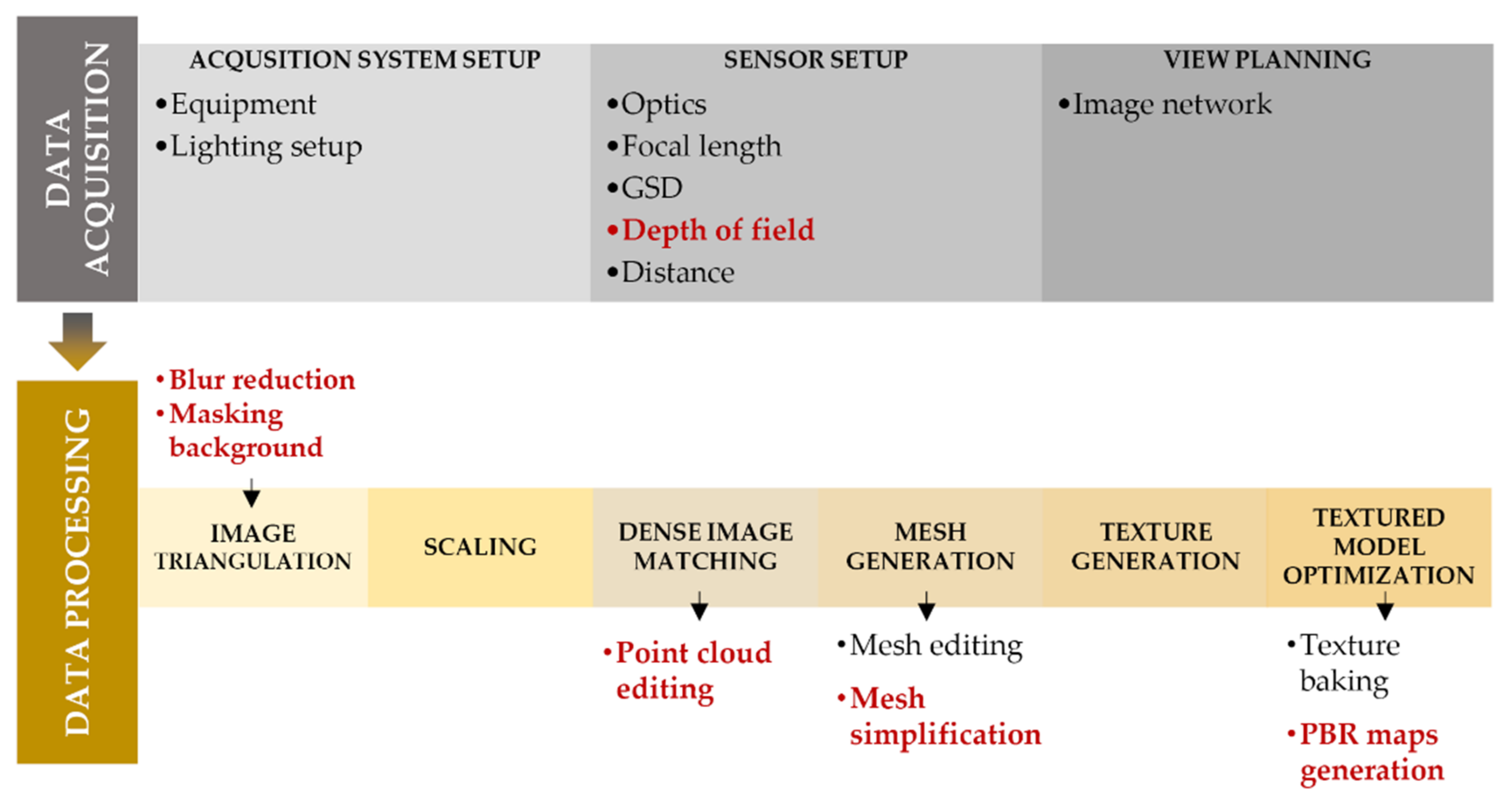
Aim and Paper Contribution

The paper reports investigations and analyses on some open issues of the photogrammetric workflow when handling the massive optimization of museum artefacts. The work deepens and extends the studies presented in Farella et al. [11] with new results useful for the 3D documentation community. In particular, some steps of the image-based digitisation pipeline are examined by performing experiments and tests:

-

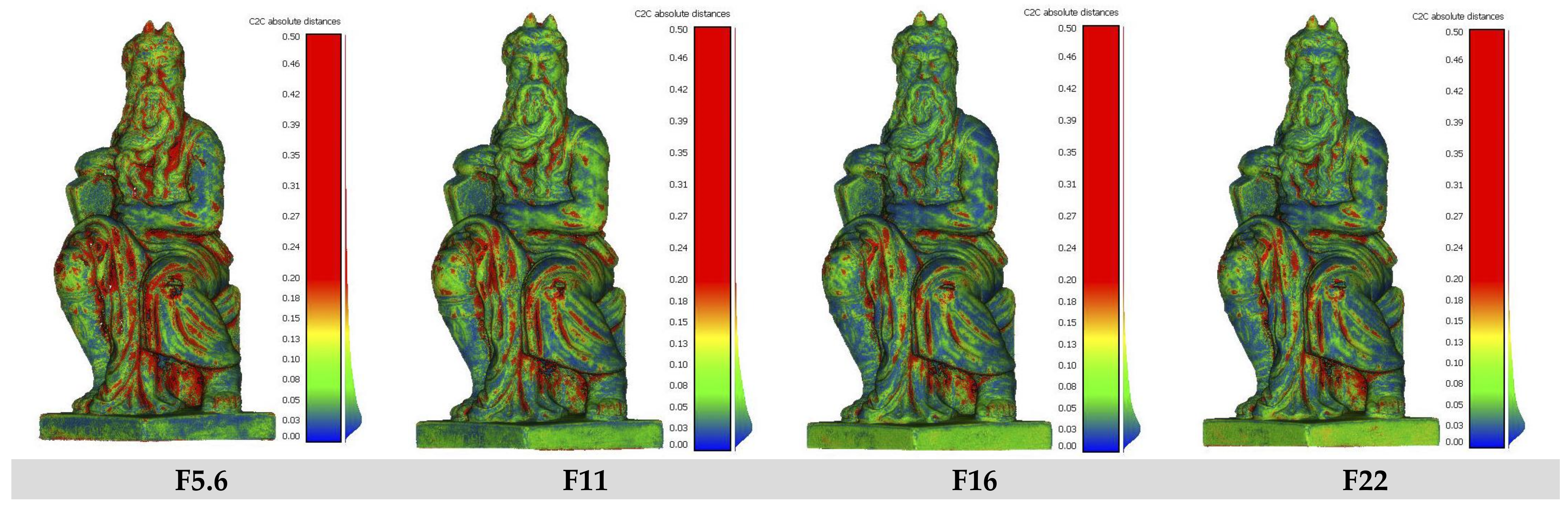
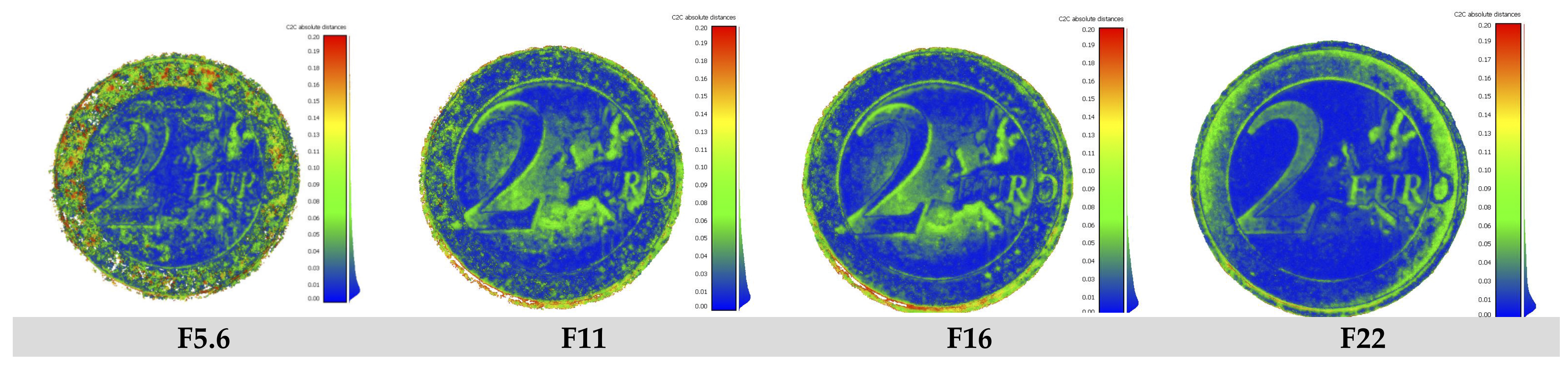
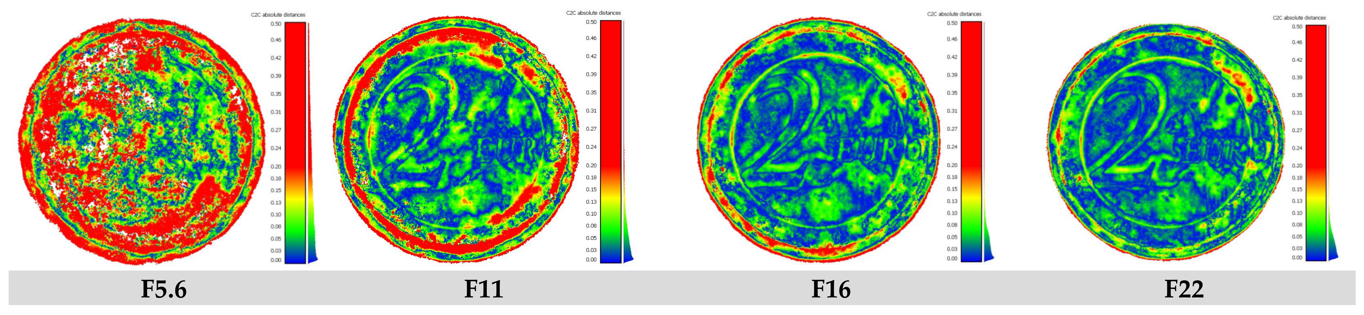
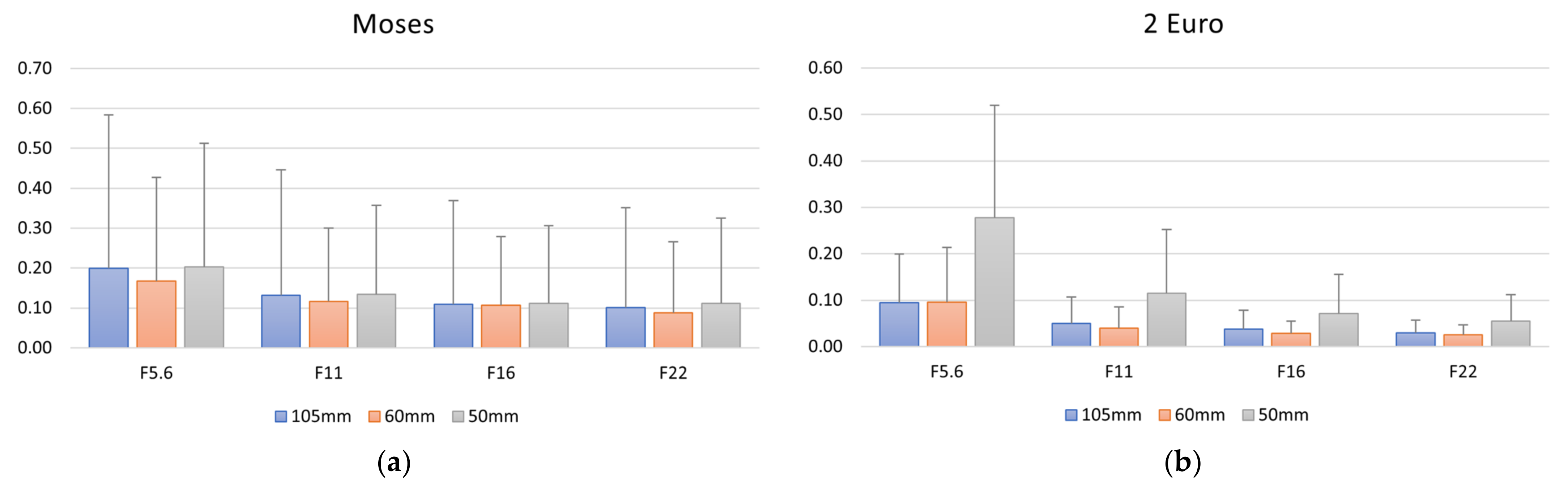
Acquisition phase: depth of field (DoF) effects when digitisation medium and small-sized artefacts are investigated. Experiments capturing images with different aperture settings and several focal lengths are proposed.

-

Data pre-processing phase: automatic image deblurring algorithms and object background masking are considered.

-

Data post-processing phase: tests are performed with point cloud cleaning solutions, while mesh optimization procedures are deepened by comparing software performance for polygons decimation. Some insights on the texture mapping are also provided.

The paper fits in the Sustainability journal section “Tourism, Culture, and Heritage” and its Special Issue on “Digital Heritage as Sustainable Resource for Culture and Tourism” as it reviews the photogrammetric pipeline—and its open issues—for the massive digitization of movable heritage artefacts. The creation of accurate and photorealistic digital collections is vital for culture and tourism, as well as for the sustainability of museums.

2. Related Works

Figure 1 introduces the general photogrammetric workflow for handling the massive digitisation of museum artefacts and create accurate digital twins but also low-weight textured 3D models for virtual museum applications, including web-based visualisation or XR solutions. The image-based pipeline consists of two leading sequences, the acquisition and processing phases, enabling the generation of 3D digital twins of heritage assets. While the system and sensor setup define the quality of the captured data, and the image network the completeness of the reconstruction, the processing step is populated by numerous phases influencing the quality of the derived 3D product. Nowadays, most processing steps can benefit from the complete automation of structure from motion and multi-view-stereo (MVS) algorithms, reducing the effort required to digitise extensive collections. Nevertheless, pre- and post-processing steps still need considerable manual engagement, and the available automatic solutions are rarely time-saving or effective for delivering high-quality products. An overview of central matters in data acquisition (Section 2.1) and processing (Section 2.2 and Section 2.3) solutions are hereafter presented. Handled problems are more deeply examined in Section 3, Section 4 and Section 5 through analyses and experiments.

2.1. Data Acquisition

The image acquisition phase is critical in massive digitisation of museum assets. Since collections are generally digitised in the available museum spaces, flexible equipment and auxiliary lights are necessary to mitigate the effects of uncontrolled image capture conditions. While for unmovable and/or large-scale objects, the acquisition inevitably suffers from the existing environmental and lighting situation, image capture can be more controlled in the case of medium and small-sized artefacts. Once the acquisition system is set (with a turntable, a uniform background, and auxiliary lights), appropriately setting up the sensors is a demanding and crucial operation to guarantee sufficient image quality. At the same time, planning an optimal camera network is essential for preventing holes and loss of geometric information, and a quite vast literature has addressed this fundamental problem [12,13,14,15,16,17,18]. The following subsection deepens one of the numerous topics related to data acquisition in museum contexts.

Depth of Field (DoF)

Selecting adequate sensor parameters is not a trivial task, since various elements during the acquisitions (Figure 1) contribute to determining the final model spatial resolution and quality. While the camera–object distance is conditioned by the need to achieve the planned GSD with available sensors and lenses, ensuring a sufficient depth of field (DoF) is crucial for returning an acceptable image sharpness, as required by image-based modelling (IBM) applications. The DoF problem is especially relevant when small artefacts are acquired with macro lenses. In addition, IBM projects require maximisation of the sensor with the object view to improve the distribution of key points and increase the number of tie points, which further influences the acquisition distance and the consequent DoF. Therefore, selecting appropriate aperture settings to solve the DoF problem is fundamental for acquiring images suitable for IBM applications.

DoF effects in 3D applications have been only partially investigated so far [19,20,21,22]. However, examining this phenomenon in different acquisition scenarios can be crucial in a massive digitisation project for meeting the expected results. While this problem has been solved for a few objects adopting the focus stacking [23,24,25,26] or shape from focus [27] techniques, these solutions are impractical when digitisation includes numerous artefacts. While the focus stacking approach requires acquiring images with shallow DoF from different focusing distances to create a new image with a longer DoF, the shape from focus technique generates sharper images from a multi-focus image sequence based on a local variance criterion.

2.2. Data Pre-Processing

Image pre-processing in photogrammetric applications is a broad topic, including colour correction and enhancement, high dynamic range (HDR) imaging, image denoising, blur correction and image masking [28,29,30]. In this work, we will focus on the object background masking and blur correction since, in our experience, they heavily condition the processing times and data quality in massive digitisation.

2.2.1. Unsharp Images

Unsharp areas on images can adversely affect the photogrammetric pipeline, preventing the correct orientation of the images, leading to less accurate point clouds and meshes, and reducing the texture quality. Unsharp regions can result from several phenomena such as the image noise for high ISO, the noise related to very small sensors, the motion blur, and the out-of-focus. When dealing with the DOF-related out-of-focus, two typical approaches rely on: (i) masking the out-of-focus areas or (ii) restoring the same level of detail as the in-focus areas.

On the masking side, Webb et al. [22] explored a solution based on the Adobe Photoshop tools ‘In-Focus Range’ and ‘Image Noise Level’, and another approach that combines depth maps, the camera–object distance and the DoF. These masking methods increased the tie point number and the quality of the textures while avoiding manual effort. Similarly, Verhoeven [31] tested several defocus algorithms for the automatic masking of huge image datasets.

Restoring out-of-focus areas is a delicate task, as changing the intensity and radiometric distribution may make it hard to identify tie points correctly or reduce their accuracy. Recently, image deblurring has been boosted from various studies on neural networks [32,33,34] and the organisation of several international challenges [35]. Furthermore, these new methods have begun to be applied in photogrammetry. For instance, Burdziakowski [36] used DeblurGANv2 [32] with UAV images to improve the 3D accuracy and the final texture of the photogrammetric reconstruction.

2.2.2. Masking Object Background

The removal of image background is a key concept in Computer Vision, and many approaches have been proposed in the last decades [37,38,39]. Modern techniques based on artificial intelligence (AI) have gradually replaced these traditional methods. The most well-known background subtraction strategy with AI is the semantic segmentation, in which the basic idea is that each pixel in an image belongs to a specific class and is labelled accordingly (i.e., background—not background).

Under the AI umbrella, unsupervised clustering, supervised machine learning (ML), and more recent and advanced deep learning (DL) algorithms can be distinguished. Grilli et al. [40] proposed an unsupervised approach for masking apple fruits based on K-means clustering [41]. A similar attempt has previously been offered by Surabhi et al. [42], where K-means was used as a pre-processing technique for face recognition. Pugazhenthi et al. [43] also proposed a valid solution for different subjects (animal, statues, person), masking backgrounds through a modified fuzzy C-means clustering algorithm [44]. In the medicine/biology field, different effective solutions for image segmentation and masking background have been released. The Ilastik tool [45], for example, introduced a supervised approach based on the random forest (RF) algorithm for biological analyses, similar to the WEKA workbench technique [46].

Regarding the DL section, UNet [47], DeepLab [48], Tiramisu [49], and Mask R-CNN [50] are the state-of-the-art methods for semantic segmentation model building. They are all designed to obtain a semantic segmentation while decreasing processing costs and increasing accuracy. Many studies have been based on the use of these models for background removal purposes [51,52,53]. In parallel, several commercial software have been released for background subtraction. Most of these tools are trained to identify people, and to the best of the author’s knowledge, there are no networks trained ad-hoc for small artefacts.

Further strategies rely on depth detection for the background separation. Beloborodov and Mestetskiy [54] proposed a “hand-crafted” method based on Kinect sensors for masking the background in RGB-D images, using depth maps as input. As presented in the following paragraphs, we propose a masking method that requires a set of RGB images as input, while the depth map is calculated downstream of a structure-from-motion (SfM) pipeline.

2.3. Data Post-Processing

Once a 3D reconstruction is obtained using MVS methods, cleaning dense point clouds before generating polygonal models is unavoidable.

2.3.1. Dense Point Cloud Cleaning

Removing noise and outliers from multi-view-stereo (MVS) reconstructions is one of the key post-processing phases that directly influences the quality of the meshes. This operation is generally highly time-consuming if handled manually. Therefore, the development of automatic dense point cloud cleaning solutions is increasingly capturing the research community’s attention [55]. Based on the adopted approach, denoising and filtering algorithms can be categorised mainly in neighbour, statistical, density and model-based [56,57,58]. The neighbourhood-based techniques assign a new position to sampling points based on some similarity measures between the sample and neighbour points (e.g., distance, curvature, angles, normal vectors, etc.) [59,60]. The statistical-based procedures identify outliers adopting the optimal standard probability distributions of a dataset [59]. These methods are quite popular, although the unpredictability of some data distributions could limit their performance. The density-based category is populated by those procedures exploiting unsupervised clustering approaches for identifying outliers. In these approaches, small clusters with a few data are identified as outliers and removed from the points set [60]. Lastly, the model or learning-based group includes all methods employing training data for learning a model and classifying outliers [61,62,63,64,65,66].

2.3.2. Mesh Simplification and Texture Mapping

Polygonal models represent the object geometry derived from the photogrammetric pipeline. Traditional surface reconstruction approaches are usually based on 3D Delaunay tetrahedralization [67,68,69] and are robust to medium levels of noise and outliers. Deep surface reconstruction (DSR) methods have been recently proposed for incorporating learned shape priors in the geometry generation [70,71,72,73]. In both cases, the artefact shape is generally reconstructed through a large number of polygons and triangles.

By reducing the number of excessive polygons, mesh simplification is a typical operation for speeding up the mapping process and facilitating interaction in engines and virtual environments [74], though it still suffers from several limitations in graphics hardware. Leading solutions exploit distance [75,76] and geometric principles [77,78], or employ energy functions [79], to perform the model simplification. Two main simplification approaches are based on vertex clustering and iterative edge collapsing [80]. Vertex clustering methods [81,82] are weak when operating on the boundaries and rely on identifying vertex clusters, which are substituted with a new single vertex representing the cluster. Representative samples are selected, adopting the average or median vertex position, or relying on error quadrics. The more performant edge collapsing methods operate iteratively, collapsing edges into vertices and trying to preserve more salient topological features. These approaches rely on error metrics as decimation criteria. Most of the decimation algorithms available today in popular 3D modelling and editing software (Meshlab, Blender, Houdini, etc.) adopt different quadric-based edge collapse method variants, relying on quadric error matrices for approximating local surfaces [83,84,85].

2.3.3. PBR Rendering Pipeline

Once the high-resolution 3D textured model is generated, some rendering techniques are available for transferring colours and more realistic physical properties to the simplified mesh reconstruction. Physically-based rendering (PBR) is a computer graphic method that provides a more realistic representation of how light interacts with surfaces [86,87,88,89]. These lighting models are (i) based on the Microfacet surface model, (i) are energy-conserving, and (iii) use a physically-based bidirectional reflectance distribution function (BRDF).

The Microfacet theory assumes that a surface is composed of small planar surfaces at a microscopic scale. Depending on the material’s roughness, they have a variable orientation that reflects light in a single direction according to the normal of the microfacet. Rough surfaces create a more diffuse reflection since the light hitting the surface is scattered in different directions. On smooth surfaces, the same reflective direction generates sharper reflections.

Energy conservation is the second theoretical pillar of PBR methods, assuming that outgoing lighting can never be more intense than the light hitting the surface.

Finally, PBR techniques use the bidirectional reflectance distribution function (BRDF), which describes a surface’s reflective and refractive properties based on microfacet theory. In particular, BRDF approximates individual light rays’ contribution to the reflected light of an opaque surface.

These techniques have recently joined the photogrammetric workflow to enhance surface information provided by the texture mapping process, creating photorealistic effects for their visualization [90]. A more detailed description of some PBR texture maps is presented in Section 5.3.

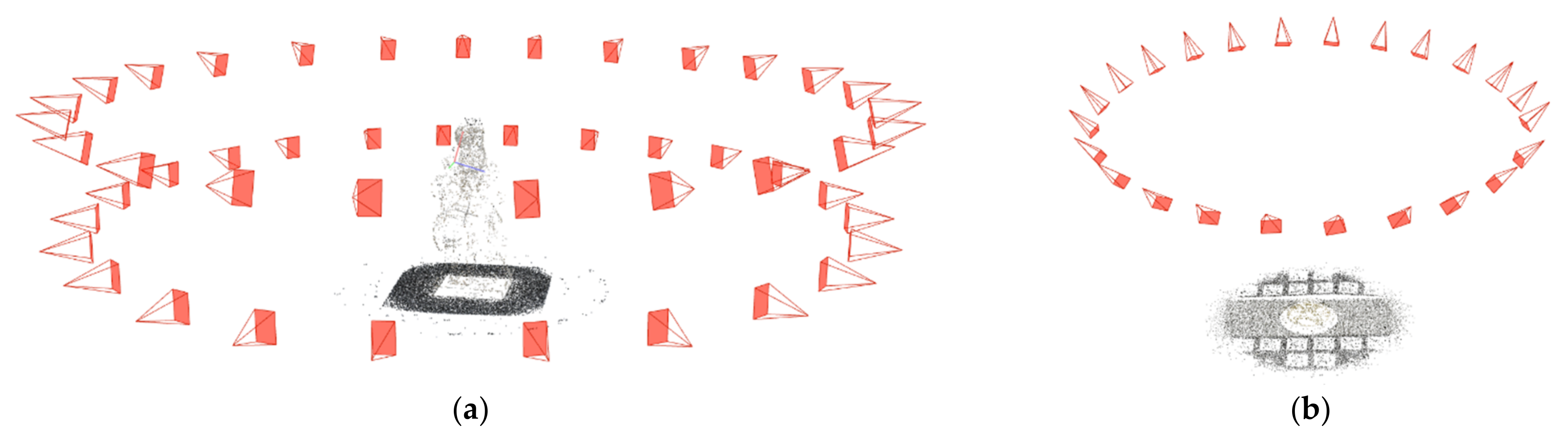
3. Image Acquisition

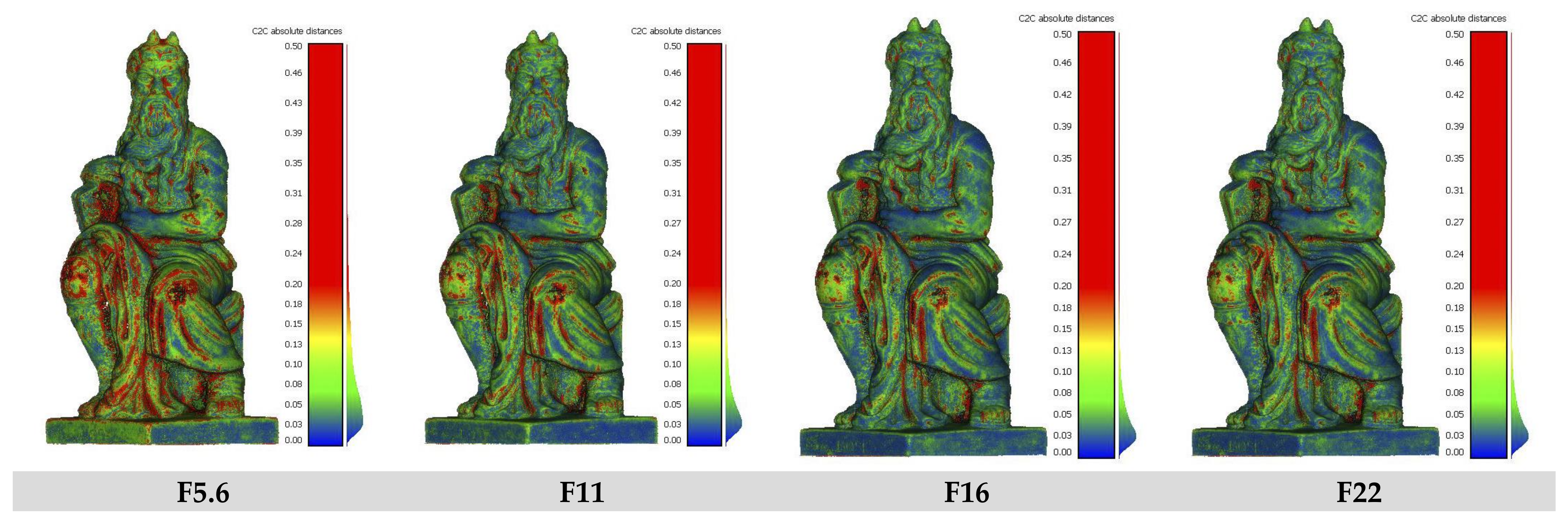
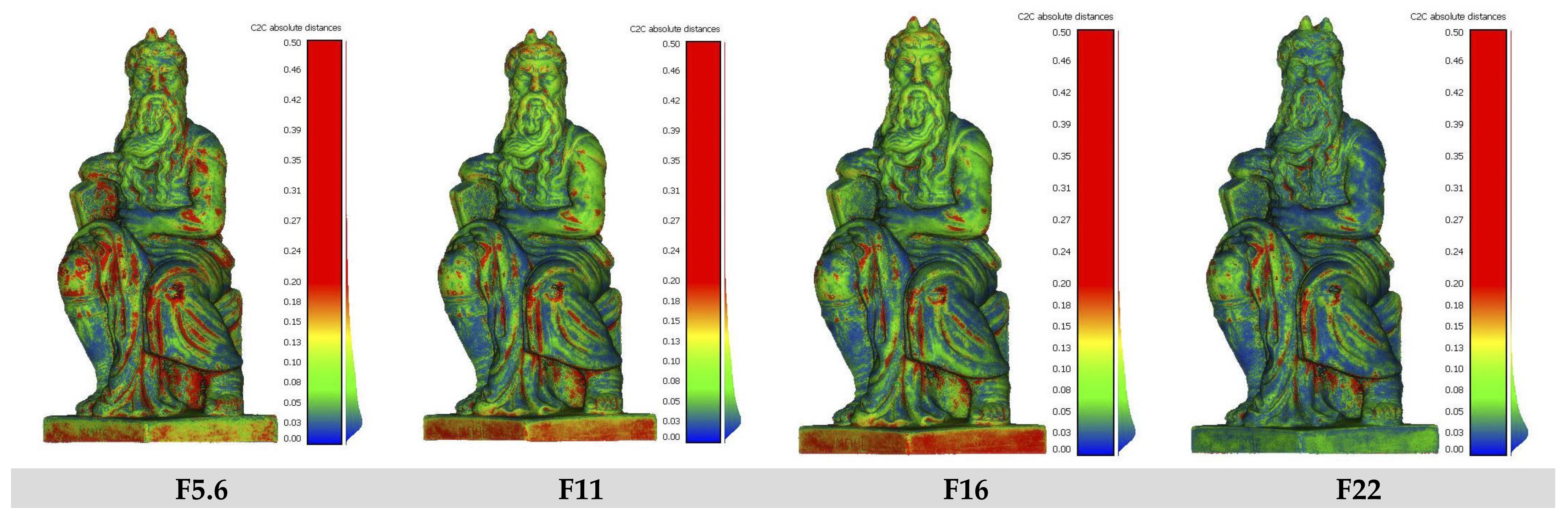
3.1. DoF Investigations

In massive digitisation of museum collections, both movable and unmovable artefacts are present, although the former are typically prevalent. In this case, and when passive techniques are employed, a proper setting of the working environment and planning of acquisition sensors (i.e., image network design) is crucial to prevent several issues in the 3D reconstruction process. Since movable artefacts are generally medium and small-sized objects, longer focal lengths and macro lenses are normally employed to produce high-resolution results. In this context, the depth of field (DoF) is a recurrent problem. In order to investigate this issue, two examples are hereafter presented.

The first object is a richly detailed statue representing Moses (6 × 6 × 15 cm), while the second is a 2 Euro coin (25 mm diameter) that simulates a tiny and reflective archaeological artefact. In both cases, 3D data acquired with a triangulation-based laser scanner, with a spatial resolution of 0.015 mm for the Moses statue and 0.01 mm for the coin, were used as ground truth. Images were acquired with a Nikon D750 full-frame camera (6016 × 4016 pixels, pixel size of 5.98 µm) coupled with three different lenses: a Sigma 105 macro f2.8, a Nikon 50 mm f1.8 and a Nikon 60 mm AF Micro f2.8. Constrained by the resolution requirements (planned GSD of 0.05 mm for the Moses and 0.02 mm for the coin), the image acquisition distances were derived and fixed for each acquisition (Figure 2). Consequently, the DoF problem can only be controlled by modifying camera aperture settings (Figure 3), considering that a higher F-number increases the DoF but could decrease the image sharpness and quality for some diffraction effects [31].

Figure 2. Camera networks and sparse point clouds for the 3D reconstruction of Moses statue (a) and the 2 Euro coin (b).

Figure 3. Some zoomed views showing the effects of the depth of field (DoF) modifying aperture settings [F5.6, F11, F16, F22] on the 2 Euro coin case and the 105 mm lens.

The Influence of DoF on 3D Reconstruction

Images were captured shooting at ISO 100 to minimize image noise, manually focusing once on the object centre, and keeping the same camera network while modifying the aperture settings (F5.6, F11, F16 and F22). Shutter speed values were changed in each acquisition to ensure a consistent and homogeneous illumination.

The Moses statue was surveyed using a rotating table and shooting every 15° from two viewpoints to prevent occlusions and reconstruct the entire object geometry (Figure 2a). Given the planned GSD of 0.05 mm, the acquisition distance was set at 500, 400, 350 mm with the 105, 60 and 50 mm lenses, respectively. Figure 4, Figure 5 and Figure 6 and Table 1, Table 2 and Table 3 show the accuracy results achieved by comparing the derived dense point clouds with the available ground truth data.

Figure 4. Cloud-to-cloud differences [mm] for the Moses statue surveyed with the 105 mm focal length and four aperture settings [F5.6, F11, F16, F22]. Range [0.00/0.50 mm].

Figure 5. Cloud-to-cloud differences [mm] for the Moses statue surveyed with the 60 mm focal length and four aperture settings [F5.6, F11, F16, F22]. Range [0.00/0.50 mm].

Figure 6. Cloud-to-cloud differences [mm] for the Moses statue surveyed with the 50 mm focal length and four aperture settings [F5.6, F11, F16, F22]. Range [0.00/0.50 mm].

Table 1. Cloud-to-cloud and cloud-to-mesh comparisons [mm] with F5.6, F11, F16 and F22 aperture settings for the Moses statue case, acquired with the 105 mm focal length. Range [0.00/0.50 mm].

F-Number	F5.6		F11		F16		F22
DoF [cm]	0.61		1.22		1.72		2.43
	Mean	St.dev.	Mean	St.dev.	Mean	St.dev.	Mean	St.dev.
C2C	0.1987	0.3851	0.1311	0.3147	0.1087	0.2607	0.1007	0.2501
C2Mesh	−0.0498	0.4296	−0.0325	0.3383	−0.0245	0.2801	−0.0260	0.2671

Table 2. Cloud-to-cloud and cloud-to-mesh comparisons [mm] with F5.6, F11, F16 and F22 aperture settings for the Moses statue case, acquired with the 60 mm focal length.

F-Number	F5.6		F11		F16		F22
DoF [cm]	1.28		2.57		3.63		5.15
	Mean	St.dev.	Mean	St.dev.	Mean	St.dev.	Mean	St.dev.
C2C	0.1669	0.2602	0.1166	0.1840	0.1063	0.1723	0.0877	0.1776
C2Mesh	−0.0057	0.3078	−0.0069	0.2162	−0.0067	0.2007	−0.0089	0.1962

Table 3. Cloud-to-cloud and cloud-to-mesh comparisons [mm] with F5.6, F11, F16 and F22 aperture settings for the Moses statue case, acquired with the 50 mm focal length. Range [0.00/0.50 mm].

F-Number	F5.6		F11		F16		F22
DoF [cm]	1.43		2.86		4.05		5.74
	Mean	St.dev.	Mean	St.dev.	Mean	St.dev.	Mean	St.dev.
C2C	0.2031	0.3092	0.1335	0.2236	0.1113	0.1943	0.1113	0.2141
C2Mesh	0.0096	0.3688	0.0006	0.2590	-0.0003	0.2223	−0.0023	0.2408

Similarly, the 2 Euro coin was captured with the same camera network but different aperture settings (Figure 2b). To obtain the planned spatial resolution of about 0.02 mm, we used a camera-to-object distance of about 200 mm with the 50 and 60 mm lenses, and a 300 mm distance with the 105 mm lens. Metric evaluation and comparisons are presented in Figure 7, Figure 8 and Figure 9 and Table 4, Table 5 and Table 6. The 50 mm focal length demonstrated to be inappropriate for this kind of application, as proved by the resulting high errors.

Figure 7. Cloud-to-cloud differences [mm] for the 2 Euro coin surveyed with the 105 mm focal length and four aperture settings [F5.6, F11, F16, F22]. Range [0.00/0.20 mm].

Figure 8. Cloud-to-cloud differences [mm] for the 2 Euro coin surveyed with the 60 mm focal length and four aperture settings [F5.6, F11, F16, F22]. Range [0.00/0.20 mm].

Figure 9. Cloud-to-cloud differences [mm] for the 2 Euro coin surveyed with the 50 mm focal length and four aperture settings [F5.6, F11, F16, F22]. Range [0.00/0.50 mm].

Table 4. Cloud-to-cloud and cloud-to-mesh comparisons [mm] with F5.6, F11, F16 and F22 aperture settings for the 2 Euro coin case, acquired with the 105 mm focal length.

F-Number	F5.6		F11		F16		F22
DoF [cm]	0.18		0.36		0.51		0.72
	Mean	St.dev.	Mean	St.dev.	Mean	St.dev.	Mean	St.dev.
C2C	0.0944	0.1047	0.0497	0.0568	0.0377	0.0410	0.0289	0.0279
C2Mesh	−0.0575	0.1282	−0.0263	0.0702	−0.0154	0.0529	−0.0033	0.0393

Table 5. Cloud-to-cloud and cloud-to-mesh comparisons [mm] with F5.6, F11, F16 and F22 aperture settings for the 2 Euro coin case, acquired with the 60 mm focal length.

F-Number	F5.6		F11		F16		F22
DoF [cm]	0.26		0.53		0.75		1.06
	Mean	St.dev.	Mean	St.dev.	Mean	St.dev.	Mean	St.dev.
C2C	0.0960	0.1174	0.0392	0.0461	0.0281	0.0266	0.0251	0.0213
C2Mesh	−0.0513	0.1424	−0.0149	0.0580	−0.0043	0.0377	−0.0007	0.0321

Table 6. Cloud-to-cloud and cloud-to-mesh comparisons [mm] with F5.6, F11, F16 and F22 aperture settings for the 2 Euro coin case, acquired with the 50 mm focal length. Range [0.00/0.50 mm].

F-Number	F5.6		F11		F16		F22
DoF [cm]	0.41		0.81		1.15		1.63
	Mean	St.dev.	Mean	St.dev.	Mean	St.dev.	Mean	St.dev.
C2C	0.2772	0.2424	0.1147	0.1372	0.0712	0.0843	0.05436	0.0578
C2Mesh	−0.0877	0.3412	−0.0121	0.1777	−0.0110	0.1085	−0.0044	0.0784

Figure 10 summarizes all results obtained for the Moses and the 2 Euro coin objects, comparing the dense reconstructions with the ground truth data.

Figure 10. Moses (a) and 2 Euro (b) case studies: mean and standard deviation of the cloud-to-cloud distances between the ground truth data and the photogrammetric models generated with three photographic lenses (105, 60 and 50 mm) and four different apertures (F5.6, F11, F16 and F22).

4. Image Pre-Processing

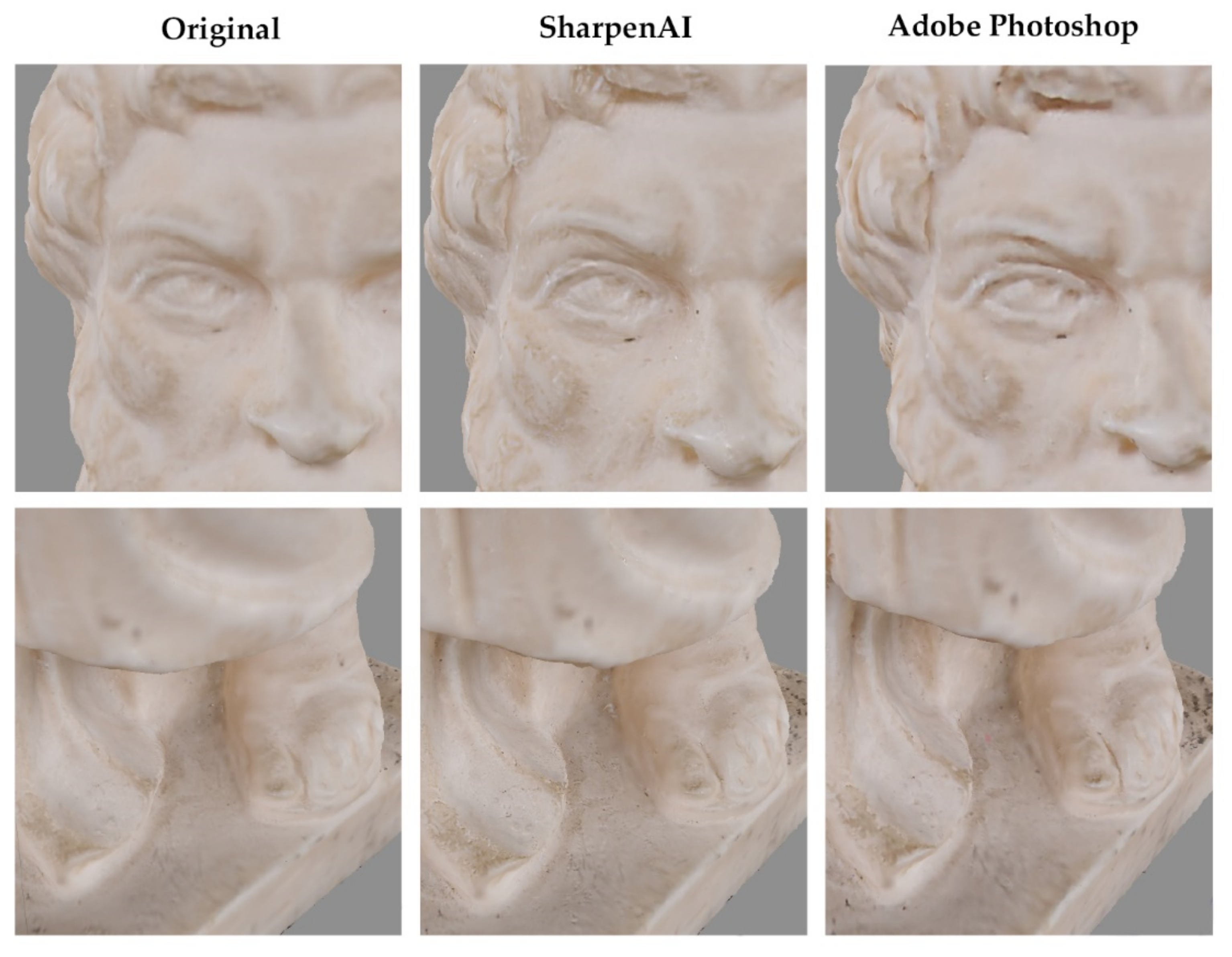
4.1. Deblur Images

4.1.1. Investigated Approaches

In the case of a limited depth of field, a significant portion of the images is generally out-of-focus. These areas negatively affect the final texture of the digitization products and should be masked. The next section reports investigations on image deblurring algorithms to increase texture quality. A well-established technique to handle blurred areas is to apply several convolution filters to images. In this work, a combination of the smart sharpen and high pass filter from Adobe Photoshop [91] is used as a reference to benchmark other methods. Tested techniques are selected based on their performance reported in literature and whose code is available: DeblurGANv2 [32] and SRN [33]. Furthermore, two commercial software were also tested: SmartDeblur [92] and SharpenAI [93].

Further tests, not reported here, demonstrated that dense 3D reconstructions achieved from deblurred images do not significantly improve the geometry and the 3D accuracy with respect to the original photos, and a better texture quality can be achieved by operating and deblurring all the single images.

4.1.2. Experiments

The selected deblurring methods were tested on various challenging images with different out-of-focus areas. The test aimed to qualitatively compare the ability of these algorithms to increase the sharpness of the blurred areas.

Results on a historical bowl (Figure 11) show that SharpenAI, a commercial learning-based deblur software, is the only method that can significantly improve image sharpness. These and other results suggest that DeblurGANv2 and SRN were mainly trained on motion blur and not on out-of-focus images. On the other hand, SharpenAI proposes two independent models. The images deblurred with SharpenAI (Figure 11) refer to only the out-of-focus model since the deblur model behaved similarly to the other two learning-based methods. Unfortunately, SharpenAI was not able to improve the texture uniformly: there is a clear improvement in sharpness on the top-right edge, while the bottom-left edge remains quite blurred.

Figure 11. Visual comparison of the performances of the investigated deblurring methods on the bowl image dataset.

A second experiment was carried out on the entire Moses dataset (105 mm lens, F5.6) to evaluate the effects of deblurring on the final texture quality. In these tests, only the more performant SharpenAI was considered among the learning-based methods, and the sharpen corrections are applied individually on each image of the dataset. Figure 12 and Figure 13 show sharpness differences between the original image and the image modified with Adobe Photoshop and SharpenAI filters. It is possible to see how SharpenAI can significantly improve the final texture compared to the original and Adobe Photoshop results.

Figure 12. Visual comparison of the deblurring capacity applied on the final texture.

Figure 13. Close view of the final Moses texture improved with the SharpenAI and Adobe methods.

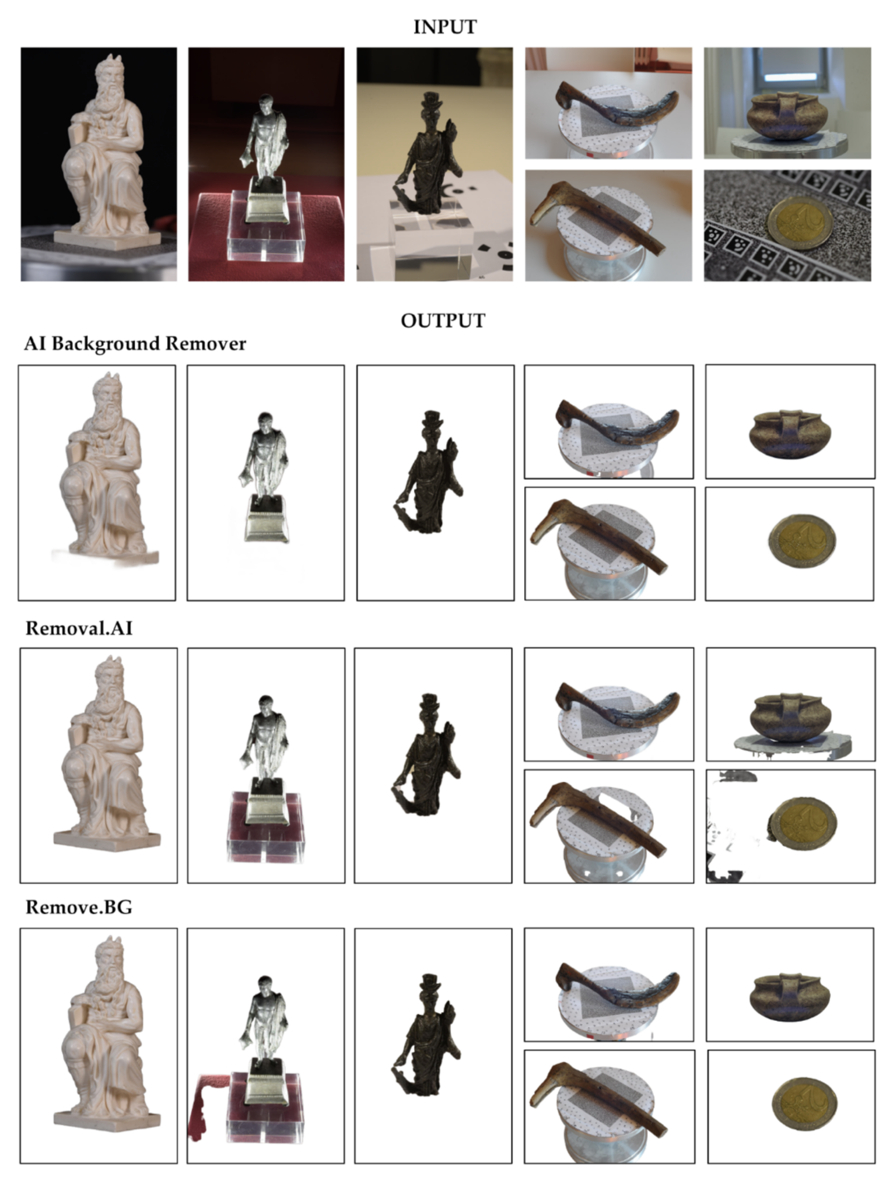
4.2. Automatic Masking Backgrounds

When medium and small artefacts are digitised using turntables and not completely uniform backgrounds, then masking object backgrounds is generally a mandatory procedure. This process is especially necessary when the object is flipped on the rotating platform during the image acquisitions for jointly orienting all images. Alternatively, sets of images captured from the same camera location and viewpoint can be processed in separate groups and then co-registered. This latter approach could introduce some unwanted registration errors in the 3D data generation process and, thus, the first approach should always be preferred. In this case, manually masking numerous images is a very onerous processing task, while automatic or semi-automatic procedures can reduce the required effort.

4.2.1. Masking Methods

Four different approaches for masking background were tested and compared. In particular, we investigated unsupervised, supervised machine learning (ML) and deep learning (DL) algorithms, as well as a depth-based approach, to identify the most rapid and accurate strategy for masking backgrounds and preserving the artefact’s shapes (Figure 14).

Figure 14. Tested approaches for background removal and mask generation. A comparison of the processing times is also reported.

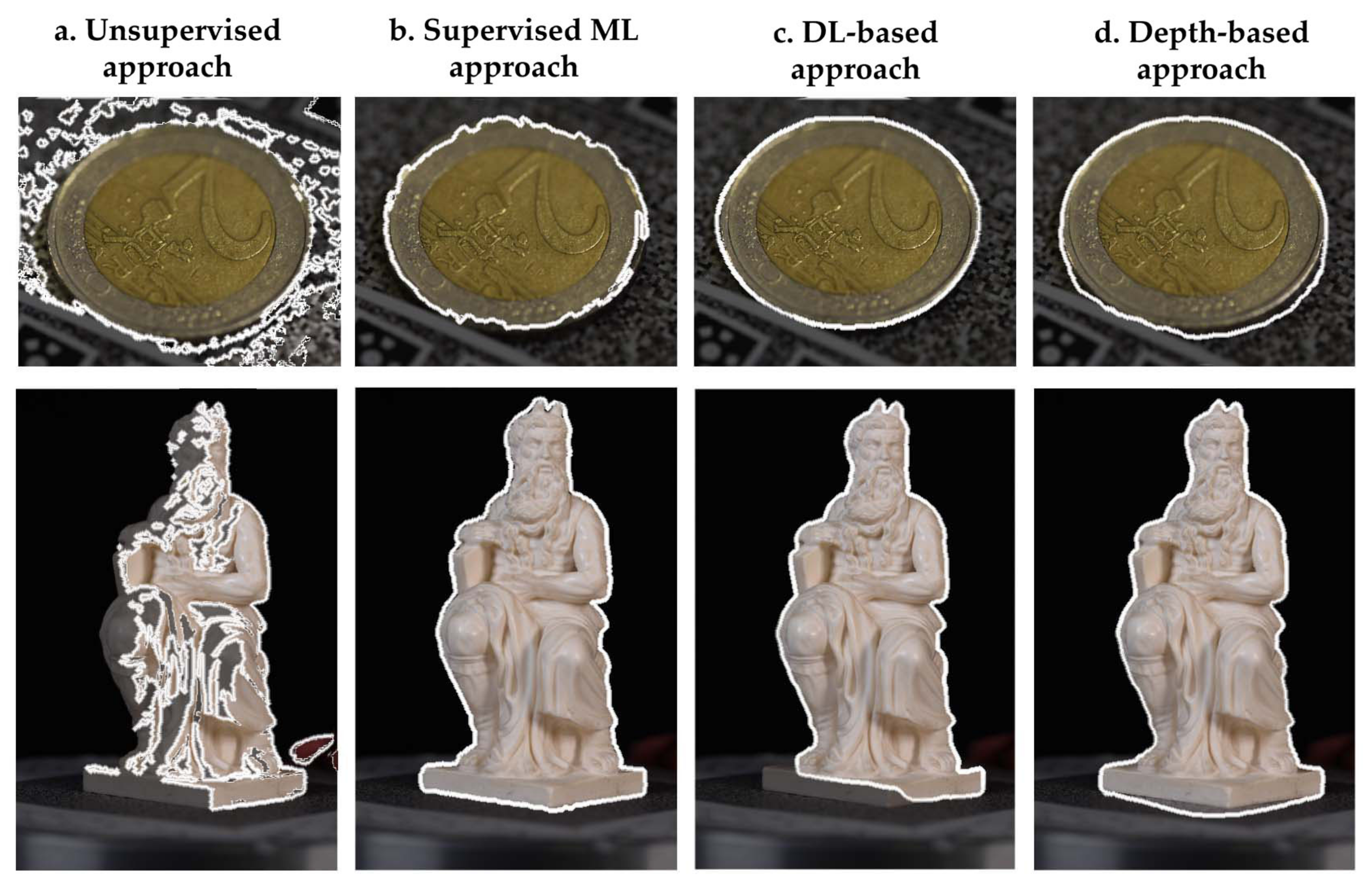
• Unsupervised learning approach: the K-means clustering approach breaks an unlabelled dataset into K groups of data points (referred to as clusters) based on their similarities. Considering that colour similarity is a fundamental feature in image segmentation, some pre-processing is applied to improve the results. In particular, RGB images are converted into the CIELAB colour space, where L* indicates the luminance and a* and b* axes respectively extend from green to blue and blue to yellow. Based on the prevailing chromatic object range, different channels can be chosen. Once the K-means algorithm is run, outputs are used to create binary masks, automatically refined through morphological processes (e.g., erosion and dilation) to remove minor undesirable components or fill small holes.
• Supervised Machine Learning approach [45]: to train the random forest algorithm and assign a class label (object or background) to each image pixel, image features and user annotations are necessary components. Colours, edge filters and texture features are used to characterise the pixel information in a multi-scale approach. Then, the model is built from a few annotated images, and the semantic segmentation is extended to the entire and/or similar datasets. Finally, the segmentation output is transformed into binary masks and further refined with morphological processes.
• Deep Learning methods: three different commercial tools for background removal have been tested and compared: AI background removal [94], removal AI [95], remove. BG [96].
• Depth map-based approach: given a set of images of an artefact, depth maps are extracted by applying photogrammetric processing at a low image resolution. Possible points belonging to the artefact background are removed from the dense reconstruction before exporting the depth maps, correcting correspondent brightness and contrast values. Then, some image processing filters are applied to the exported depth maps, such as (i) a Gaussian blur filter, or Gaussian smoothing, to minimise image noise, and (ii) a Posterisation filter to reduce the amount of image colours while restoring sharper edges. In the developed procedure, the post-processing phase is run in a single round until mask generation. It is also worth noting that depth maps could be quickly predicted using monocular techniques and deep learning networks [97]. However, while promising for dealing with the typical ill-posed problem, these approaches are not well suited for masking artefact datasets, and further research in this field is required.

4.2.2. Masking Experiments

The aforementioned masking approaches were tested over a wooden bowl, the previously presented Moses statue and the 2 Euro coin (Figure 14 and Figure 15). When objects and background are clearly distinguishable, as for the bowl case study, the unsupervised procedure can be effective and simple for the operator (Figure 14). On the other hand, artefacts often share a similar pattern or colour with the background setting. In these cases, the algorithm will incorporate some parts of the background in the same segment, influencing the production of accurate masks (Figure 15a).

Figure 15. Masking results achieved with four different approaches. Unsupervised approach with K-means algorithm (a); supervised ML approach by Ilastik tool (b); DL-based approach by AI background removal (c), depth-based approach (d).

When using supervised learning methods, patches and features for training the classifier and generating the dataset model should be carefully picked. Once the efficiency of the pre-trained model is proven, mask production is quick, manual work is reduced, and results are generally satisfactory (Figure 15b). In the 2 Euro coin case, the wavy outline of the mask is influenced by blurry effects on the image.

The DL- and depth-based approaches returned satisfying results for both the coin and the Moses object (Figure 15c,d).

Further tests and analyses on DL-based background removal methods with more complex objects are shown in Figure 16. Even if the employed tools are built for recognising people, they can still perform well with heritage objects, such as small statues (a typical example of transfer learning). On the contrary, when the rotating table appears in the scene, it is frequently kept in the final output, creating issues in the 3D reconstruction when objects are moved and flipped during the acquisitions.

Figure 16. Results with DL-based background removal methods applied to different heritage artefacts.

5. Data Post-Processing

5.1. Automatic Point Clouds Cleaning

5.1.1. Investigated Denoising Methods

As presented in Section 2.3.1, numerous methods have been already implemented for handling the crucial dense point clouds editing and cleaning process. In [10] three approaches were tested and further investigations on their denoising capabilities are hereafter proposed. The analyses are focused on one popular statistical method, a distance-based approach and two novel learning-based techniques:

• The Statistical Outlier Removal (S.O.R.): it is a popular and efficient method implemented in Cloud Compare [98] as part of the Point Cloud Library (PCL, [99]). Once the number of points to be considered as neighbours is set, using a K-means nearest neighbours approach [100], the average distance of each sampling point to its neighbours is calculated. Points outside the range defined by the global average distances and standard deviation are recognized as outliers and removed from data.
• PointCleanNet (PCNet—[64]): as one of the pioneering learning-based denoising approaches, this method exploits an architecture adapted from PCPNet [101] for locally estimating 3D shape point cloud characteristics. In its implementation, a first module allows removing detected outliers, while some correction vectors are later calculated for projecting noisy points on the estimated clean surface.
• Score-based denoising [66]: it relies on a neural network architecture that employs the estimated score of some point distributions to perform gradient ascent and denoise the point cloud. A noisy point cloud distribution is treated as a set of noise-free points p(x) convolved with a noise model n. The (p*n)(x) mode is, in this case, the underlying clean surface. The log-likelihood of each point is increased via gradient ascent and each point position is iteratively updated, while outliers are neither detected nor removed.

5.1.2. Denoising Experiments

In the investigations, a synthetic bowl (40 cm diameter) was modelled, generating three levels of random noise for verifying the cleaning capabilities of the aforementioned denoising methods. The bowl reproduces shapes and geometries that typically can be found among museum collections. The three levels of noise correspond respectively to the 0.5, 1, 2% of the bowl diameter. Figure 17 and Figure 18 show the metric and visual evaluation of the denoising results. Similar to [10], results confirm the good performance of the statistical-based method and some unsolved issues with the learning-based approaches when the level of noise increases.

Figure 17. Average cloud-to-cloud distance [mm] between the denoised models and the ground truth data (the original bowl surface). Results with three increasing levels of noise (0.5%, 1%, 2%) are reported.

Figure 18. Visual comparison of the denoising results applied to different noise levels. In red, the ground truth surface. In white, the denoised dense point clouds. Where white is prevalent in the figures, a less denoising capacity is notable.

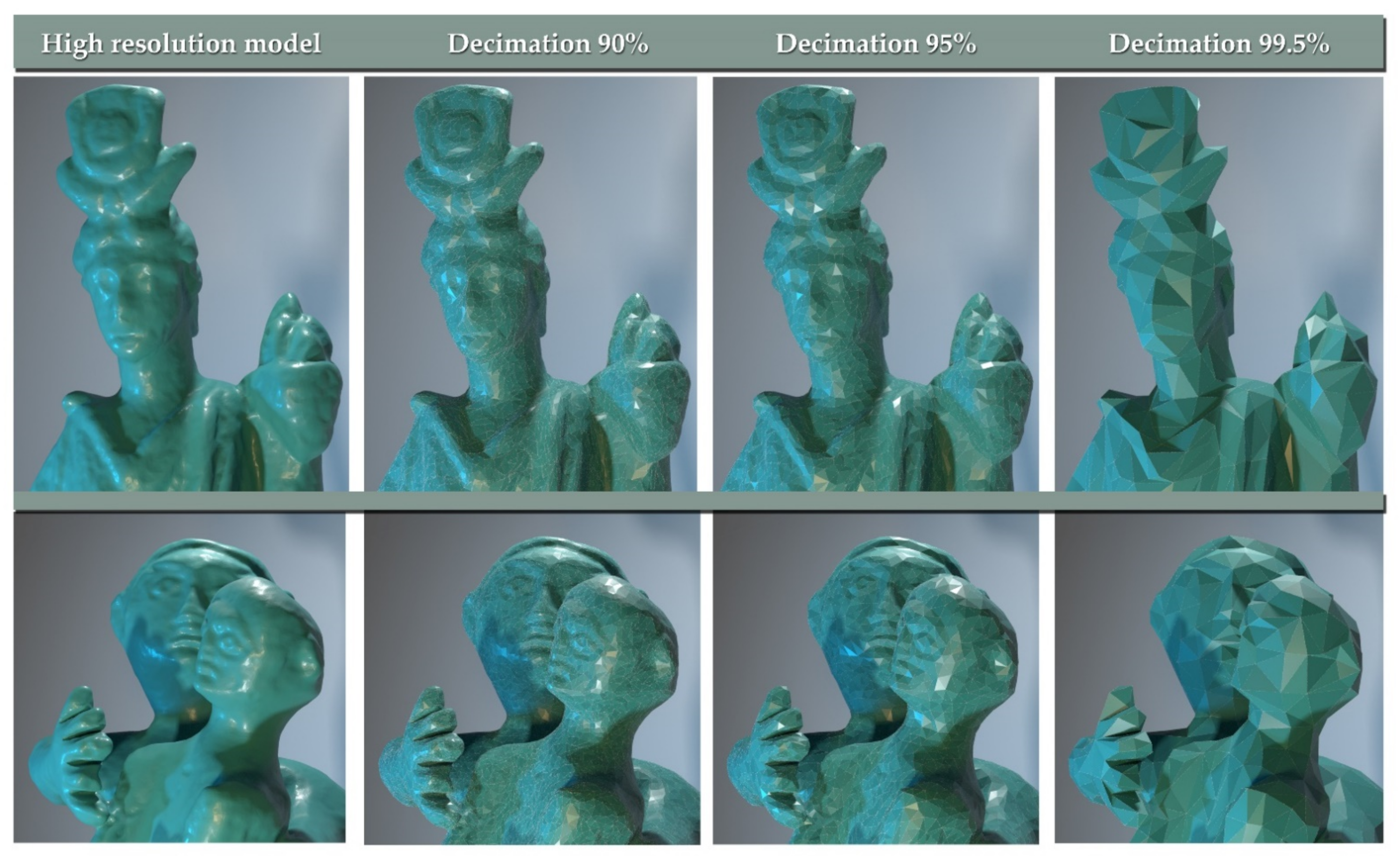
5.2. Mesh Simplification

5.2.1. Investigated Tools for Mesh Decimation

Mesh simplification is a common practice for minimising model size by reducing the number of faces while preserving the shape, volume, and boundaries. The simplification process should always compensate for the required complexity reduction, a sufficient object geometry representation and salient features preservation. Criteria for mesh decimation are generally user-defined, selecting the reduction method (working on the number of vertices, edges, or triangles) and the reduction target. Several commercial and open-source editing and modelling software include a mesh simplification module for handling this post-processing task efficiently. Most of these solutions rely on edge collapsing methods (Section 2.3.2) for removing edges, triangles and vertices, adopting error metrics for measuring the similarity of the reduced model with respect to the original one.

5.2.2. Decimation Tests

The number of polygons of two high-resolution 3D models (two small bronze statuettes) was decimated by testing three significant reduction percentages (90%, 95%, 99.5%) in Blender, Houdini and Meshlab. The high-resolution model of a bronze representation of goodness Iside (ca 6 cm height) counts ca 430,000 faces, while the bronze reproduction of a “Mother with the child” (ca 12 cm heigh) has ca 570,000 faces (Figure 19).

Figure 19. Examples of mesh simplification results with three levels of decimation: the Iside 3D model (middle row) decimated with Blender and the Mother with Child 3D model (bottom row) decimated with Houdini. Differences in the decimation outputs are hardly appreciable.

A metric evaluation of the simplification processes with different levels of decimation is reported in Figure 20, where the original high-resolution polygonal model is compared to the reduced meshes. More relevant differences are evident with the smaller statuette (Iside case study).

Figure 20. RMSE of decimated surfaces compared with the original high-resolution model. On the left, the results of the Iside data, while, on the right, errors achieved testing the Mother with Child models. In both cases, three percentages of decimation were investigated.

5.3. Texture Mapping

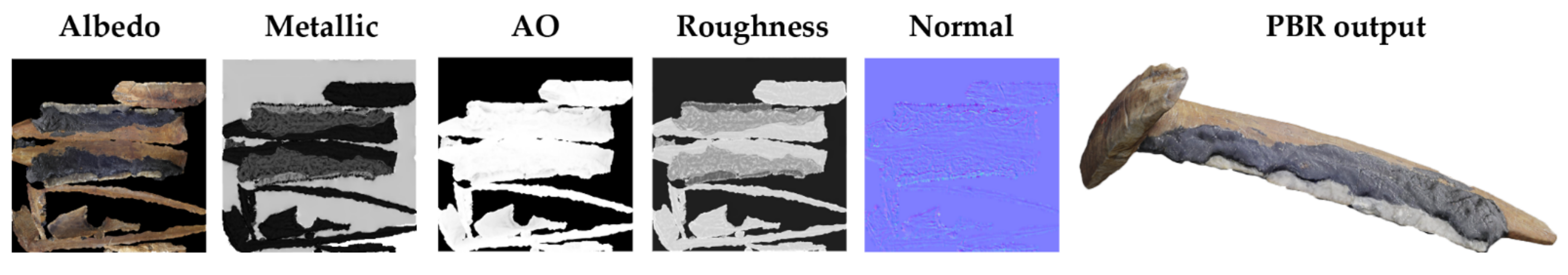
5.3.1. PBR Texture Maps

In a PBR pipeline (Section 2.3.3), the most common textures generated for simulating the properties of the physical object are usually:

• Albedo map: this texture contains the base colour information of the surface or the base reflectivity when texels are metallic. Compared to the diffuse map, the Albedo map does not contain any lighting information. Shadows and reflections are added subsequently and coherently with the visualisation scene.
• Normal map: this is a texture map containing a unique normal for each fragment to describe irregular surfaces. Normal mapping is a common technique in 3D computer graphics for adding details on simplified models.
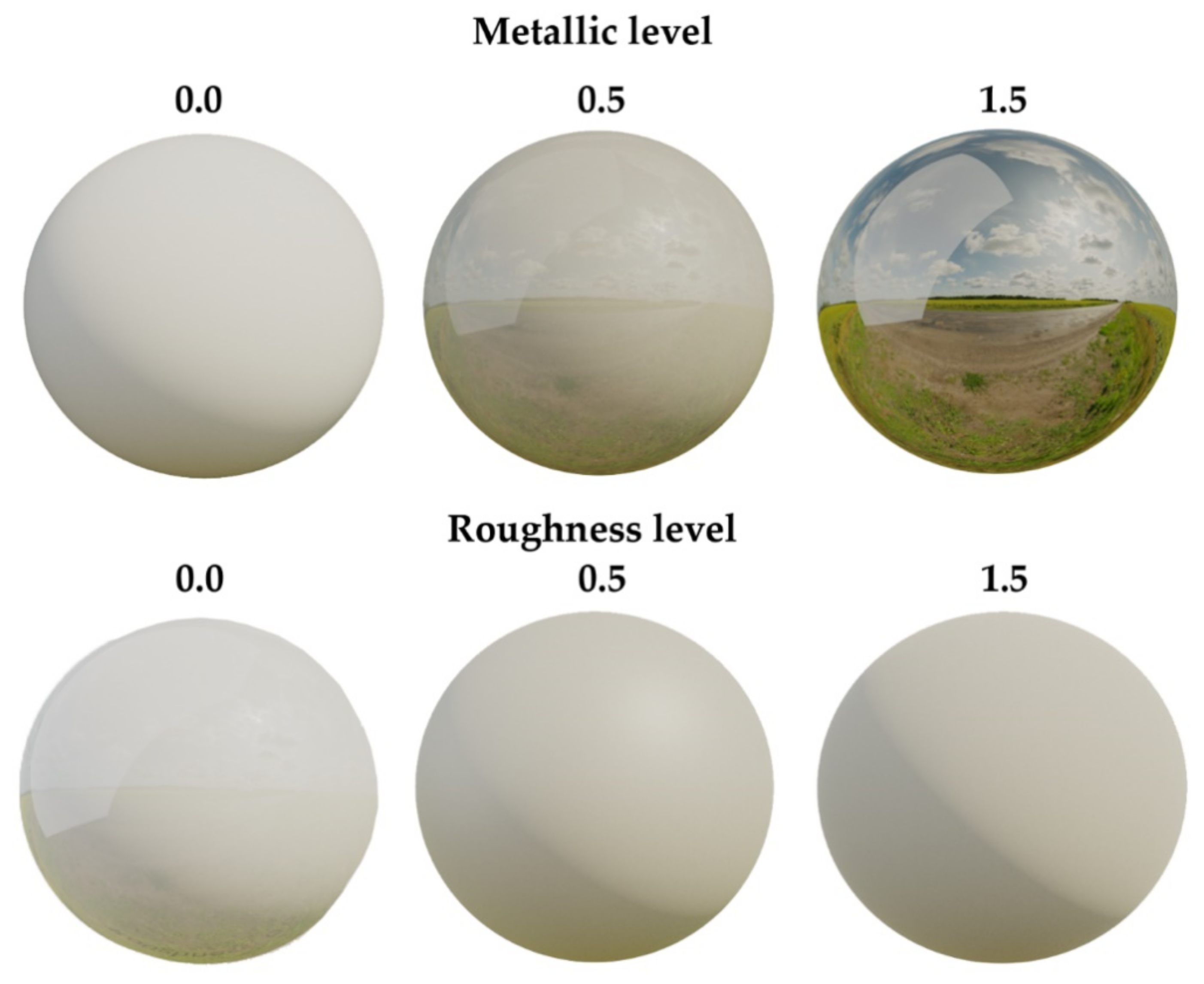
• Metallic map: this map represents whether each texel is metallic or not. It is a black and white texture acting as a mask for defining whether the texture behaves as metal or not.
• Roughness map: this texture map defines how rough each texel is, influencing the light diffusion and direction, while the light intensity remains constant.
• Ambient Occlusion map (AO): this map is used to provide indirect lighting information, introducing an extra shadowing factor for enhancing the geometry surface. The map is a grayscale image, where white regions indicate areas receiving all indirect illumination.
• The next section presents some texture outputs and their capability of enhancing the object visualisation.

5.3.2. Generating Texture Maps

Most commercial and open-source photogrammetric software include modules for texture mapping and MVS-texturing. Once the high-resolution textured model and its simplified geometry are generated, the information needs to be transferred from the high to the low-poly reconstruction. This process, implemented and available in several mesh editing software, is called baking. The colour and material information of the highly detailed model, stored in texture files, are assigned to the optimised geometry from the baking process. Most of the texture maps needed for the PBR pipelines are automatically generated by photogrammetric software (usually the Albedo and Normal maps), or they can be created and modified in image or mesh editing tools (e.g., Photoshop, Gimp, Agisoft Delighter, Blender, Quixel Mixer, etc.). The Albedo map, for example, is generally obtained by processing the diffuse map (the typical photogrammetric output) and removing shadows and lights. Some examples of generated PBR texture maps (Figure 21) and their capability of reproducing material properties (Figure 22 and Figure 23) are shown below.

Figure 21. An example of different PBR texture maps generated for the final optimised geometry of a museum artefact.

Figure 22. An example of how materials can be differently perceived by acting, for example, on the metallic and roughness values.

Figure 23. Some examples of enhanced geometric details perception using the occlusion (upper images) and normal (bottom) maps in the PBR rendering pipeline.

6. Discussions

6.1. Image Acquisition

As presented in Section 3.1, depth of field (DoF) is a recurrent problem, especially when digitising medium and small-sized artefacts and a high level of detail is required in the final 3D reconstruction. Experiments focused on assessing the achievable dense reconstruction quality in several acquisition scenarios, testing three long focal lengths (105, 60 and 50 mm) and several aperture settings for digitizing two different-sized objects. With the bigger object, the Moses statue, a general improvement of error metrics by increasing the aperture settings is clear, with a more relevant difference among the first three F-stop (F5.6, F11, F16). This trend can be observed with all the tested focal lengths, confirming that a lower image quality with higher F-numbers does not affect the 3D reconstruction outputs, although error improvements are less notable between the last two F-stops (F16–F22). Similarly, for the 2 Euro coin, relevant differences can be found by increasing the aperture values. In this case, the higher reconstruction errors of the 50 mm proved that this focal length is inadequate for digitising very small artefacts.

6.2. Image Pre-Processing

Among the methods tested for restoring out-of-focus areas (Section 4.1), only the commercial software SharpenAI proved to improve image sharpness significantly, even if these enhancements can occur unevenly. The other deep-based approaches, returning outstanding results in the literature for motion-blurred images, fail to achieve satisfactory outputs for out-of-focus areas, probably requiring an ad-hoc re-training of its neural network model.

Four different background masking approaches were also tested and compared in Section 4.2. The unsupervised method based on a K-means algorithm proved to effectively work in a museum context only when the background is uniform and in contrast to the detected object. When using a standard machine learning approach, the model requires us to specify what to detect and classify in every change of scene/object. On the contrary, when choosing a deep learning approach for background masking, the image segmentation performance depends on the amount and type of training data behind the model. Most of the available commercial software are trained on dataset capturing people. Hence, they are not suitable for segmenting most museum artefacts, although they can perform well with some objects (e.g., statues). On the other hand, considering the possibility of integrating new labelled datasets within the training, it is reasonable to affirm that the DL-based approach represents the best solution in terms of quality of the results and the manual effort required. Finally, the depth map processing proved to deliver remarkably accurate masks, although the current pipeline requires longer processing times for providing the desired results.

6.3. Data Post-Processing

Some data editing processes are considered in Section 5, where experimental results on traditional and innovative point cloud denoising methods (Section 5.1), comparisons of some mesh simplification outputs (Section 5.2), and examples of an optimal rendering pipeline (Section 5.3) are presented.

Point cloud denoising experiments compared the cleaning performance of the statistical outlier removal (S.O.R.) filter, a well-known statistical and distance-based method, and two novel learning-based approaches, PointCleanNET and score-based denoising. Some preliminary investigations on their denoising capabilities have been presented in Farella et al. [11], highlighting the need for further analyses. In Section 5.1, noise reduction is evaluated using a synthetic bowl’s cleaned geometries as a reference and adding three levels of random noise. The bowl was modelled to simulate a typical artefact shape and dimension in museum collections digitisation. Visual and metric achievements partially confirm previous results on a synthetic cube case. The S.O.R. filter outperformed the other methods with all the levels of noise tested. S.O.R. outputs are, however, strongly dependent on the user-defined number of nearest neighbours (the KNN approach). If this number is not correctly set, point clouds can be aggressively filtered. In this case, several tests were performed to find optimal neighbour values, considering the density of the generated point cloud and the quality of the output for avoiding holes and geometry losses. The other two learning-based methods basically confirmed their good performance when operating on objects affected by low levels of noise. The methods proved to be inefficient by increasing this level, especially considering the additional computation time required for the processing. The lack of a noise removal action, in the score-based case, justifies the worse error performance when the noise is higher, while the PointCleanNET shows a more linear behaviour.

Mesh simplification experiments, presented in Section 5.2, focused on verifying the quality of decimation outputs, testing three tools commonly used for handling this process. High-resolution model simplification, reducing the number of polygons and adopting three accentuate percentages of reductions, was performed with Meshlab, Blender and Houdini. While visually, decimation differences among the methods are hardly identifiable, metric discrepancies between the high-resolution and simplified geometries can be compared. Tests on the first smaller object, the bronze statuette of Iside, show more accentuated differences among the reduction outputs, with Blender metrics outperforming the other methods. Experiments on the Mother with Child statuette returned more homogeneous and quite similar results. Meshlab outputs are, also in this case, slightly worse compared to the other tools, while Houdini proved to be more efficient with the lower percentage of reduction. However, all the tested software were able to preserve quite optimal object geometries up to the 90% decimation, mostly sufficient for managing the models in other engines.

Section 5.3 introduced some key concepts and operations currently handled in the digitisation practice to enhance the quality 3D models visualisation but are still scarcely presented in photogrammetry-based publications. The section presented PBR materials for the rendering pipeline and some examples of texture maps generated from the photogrammetric pipeline or extracted through further processing operations. The geometry enhancement and more realistic visualisation of model surface details were also shown using, as an example, the Occlusion or the Normal maps. This section mainly presented how computer graphics techniques have currently joined and expanded the traditional photogrammetric pipeline, deeply contributing to improving the photorealism of 3D digital replicas.

7. Conclusions

Through tests and experimental results, this paper explored some key steps of the photogrammetric digitisation workflow for the digitization of museum objects. The creation of accurate and photorealistic 3D heritage contents boosts the sustainability of cultural heritage enlarging access and visualization.

The explored topics and operations are, based on a vast experience in massive museum digitisation, critical for determining the quality of the reconstruction outputs and the time needed for data processing.

Acquisition experiments and simulation of capturing scenarios show that higher aperture settings (although the lower image quality and the higher acquisition times) are preferable for limiting the DoF problem with medium and small artefacts and achieving more accurate and less noisy reconstructions. DoF is a recurrent issue when acquisition distance is bounded by high spatial resolutions required and the need to maximise the object view for supporting the IBM pipeline.

Some insights on the pre-processing phase were presented, focusing on exploring some deblurring techniques and proposing new methods for speeding up the image background masking. Despite the broad interest of the research community on the image sharpness topic, tested networks proved that ad-hoc training on the out-of-focus task rather than on motion blur is required. Regarding background removal and masking generation, different approaches have been taken into consideration. Except for the clustering method, both the supervised machine and deep learning, and the depth-based strategies, are satisfying solutions for accelerating an otherwise time-consuming task. Further investigations are planned for improving the accuracy results, training a convolutional neural network (CNN) with ad hoc images. Some of the presented masking methods are available on the 3DOM-FBK Github page [102].

Lastly, some data editing and optimisation steps were also examined in the articles. Three automatic denoising procedures were tested to analyse the quality of derived outputs and compare their cleaning performance. All the methods returned cleaner point clouds with a low level of noise, although learning-based approaches required higher computational time. The more traditional method, the S.O.R. filter, outperformed the more recent denoising techniques with a more significant level of noise and outliers, properly setting the number of neighbour points for the statistical and density analyses. Moreover, mesh decimation outputs from three popular tools were tested for verifying their capability of preserving artefacts shape. All tested tools proved to keep objects topology efficiently up to a fairly high decimation percentage. Finally, the last part of the work presented some inputs on the PBR materials for enhancing geometry and details. These rendering techniques, developed in the computer graphics field, still need to be further investigated by the photogrammetric community for exploiting their potential in image-based reconstruction pipelines.

References

- Tausch, R.; Domajnko, M.; Ritz, M.; Knuth, M.; Santos, P.; Fellner, D. Towards 3D Digitization in the GLAM (Galleries, Libraries, Archives, and Museums) Sector—Lessons Learned and Future Outlook. IPSI Trans. Internet Res. 2020, 16, 45–53. [Google Scholar]
- European Commission Commission Recommendation of 27 October 2011 on the Digitisation and Online Accessibility of Cultural Material and Digital Preservation (2011/711/EU); 2011. Available online: https://eur-lex.europa.eu/LexUriServ/LexUriServ.do?uri=OJ:L:2011:283:0039:0045:EN:PDF (accessed on 17 February 2022).
- Network of European Museum Organisations Working Group on Digitilisation and Intellectual Property Rights, Digitisation and IPR in European Museums; 2020. Available online: https://www.ne-mo.org/fileadmin/Dateien/public/Publications/NEMO_Final_Report_Digitisation_and_IPR_in_European_Museums_WG_07.2020.pdf (accessed on 17 February 2022).
- Remondino, F.; Menna, F.; Koutsoudis, A.; Chamzas, C.; El-Hakim, S. Design and Implement a Reality-Based 3D Dig-itisation and Modelling Project. In Proceedings of the 2013 Digital Heritage International Congress (Digital Heritage), Marseille, France, 28 October–1 November 2013; Volume 1. [Google Scholar]
- Mathys, A.; Brecko, J.; van den Spiegel, D.; Semal, P. 3D and Challenging Materials. In Proceedings of the IEEE 2015 Digital Heritage, Granada, Spain, 28 September–2 October 2015; Volume 1, pp. 19–26. [Google Scholar]
- Cultlab3d. Available online: https://www.cultlab3d.de/ (accessed on 17 February 2022).
- Witikon. Available online: http://witikon.eu/ (accessed on 17 February 2022).
- The British Museum. Available online: https://sketchfab.com/britishmuseum (accessed on 7 February 2022).
- Menna, F.; Nocerino, E.; Morabito, D.; Farella, E.M.; Perini, M.; Remondino, F. An Open Source Low-Cost Automatic System for Image-Based 3D Digitization. ISPRS Int. Arch. Photogramm. Remote Sens. Spat. Inf. Sci. 2017, 42, 155. [Google Scholar] [CrossRef] [Green Version]
- Gattet, E.; Devogelaere, J.; Raffin, R.; Bergerot, L.; Daniel, M.; Jockey, P.H.; de Luca, L. A Versatile and Low-Cost 3D Acquisition and Processing Pipeline for Collecting Mass of Archaeological Findings on the Field. ISPRS Int. Arch. Photogramm. Remote Sens. Spat. Inf. Sci. 2015, 40, 299. [Google Scholar] [CrossRef] [Green Version]
- Farella, E.M.; Morelli, L.; Grilli, E.; Rigon, S.; Remondino, F. Handling Critical Aspects in Massive Photogrammetric Digitization of Museum Assets. ISPRS Int. Arch. Photogramm. Remote Sens. Spat. Inf. Sci. 2022, 46, 215–222. [Google Scholar] [CrossRef]
- Fraser, C.S. Network Design Considerations for Non-Topographic Photogrammetry. Photogramm. Eng. Remote Sens. 1984, 50, 1115–1126. [Google Scholar]
- Hosseininaveh, A.; Serpico, M.; Robson, S.; Hess, M.; Boehm, J.; Pridden, I.; Amati, G. Automatic Image Selection in Photogrammetric Multi-View Stereo Methods. In Proceedings of the 13th International Symposium on Virtual Reality, Archaeology, and Cultural Heritage, incorporating the 10th Eurographics Workshop on Graphics and Cultural Heritage, VAST—Short and Project Papers, Brighton, UK, 19–21 November 2012. [Google Scholar]
- Alsadik, B.; Gerke, M.; Vosselman, G. Automated Camera Network Design for 3D Modeling of Cultural Heritage Objects. J. Cult. Herit. 2013, 14, 515–526. [Google Scholar] [CrossRef]
- Ahmadabadian, A.H.; Robson, S.; Boehm, J.; Shortis, M. Stereo-Imaging Network Design for Precise and Dense 3d Reconstruction. Photogramm. Rec. 2014, 29, 317–336. [Google Scholar] [CrossRef]
- Voltolini, F.; Remondino, F.; Pontin, M.G.L. Experiences and Considerations in Image-Based-Modeling of Complex Architectures. ISPRS Int. Arch. Photogramm. Remote Sens. Spat. Inf. Sci. 2006, 36, 309–314. [Google Scholar]
- El-Hakim, S.; Beraldin, J.A.; Blais, F. Critical Factors and Configurations for Practical Image-Based 3D Modeling. In Proceedings of the 6th Conference Optical 3D Measurements Techniques, Zurich, Switzerland, 23–25 September 2003; pp. 159–167. [Google Scholar]
- Fraser, C.S.; Woods, A.; Brizzi, D. Hyper Redundancy for Accuracy Enhancement in Automated Close Range Photogrammetry. Photogramm. Rec. 2005, 20, 205–217. [Google Scholar] [CrossRef]
- Menna, F.; Rizzi, A.; Nocerino, E.; Remondino, F.; Gruen, A. High resolution 3d modeling of the behaim globe. ISPRS Int. Arch. Photogramm. Remote Sens. Spat. Inf. Sci. 2012, 39, 115–120. [Google Scholar] [CrossRef] [Green Version]
- Sapirstein, P. A High-Precision Photogrammetric Recording System for Small Artifacts. J. Cult. Herit. 2018, 31, 33–45. [Google Scholar] [CrossRef]
- Lastilla, L.; Ravanelli, R.; Ferrara, S. 3D High-Quality Modeling of Small and Complex Archaeological Inscribed Objects: Relevant Issues and Proposed Methodology. ISPRS Int. Arch. Photogramm. Remote Sens. Spat. Inf. Sci. 2019, 4211, 699–706. [Google Scholar] [CrossRef] [Green Version]
- Webb, E.K.; Robson, S.; Evans, R. Quantifying depth of field and sharpness for image-based 3d reconstruction of heritage objects. ISPRS Int. Arch. Photogramm. Remote Sens. Spat. Inf. Sci. 2020, 43, 911–918. [Google Scholar] [CrossRef]
- Brecko, J.; Mathys, A.; Dekoninck, W.; Leponce, M.; VandenSpiegel, D.; Semal, P. Focus Stacking: Comparing Commercial Top-End Set-Ups with a Semi-Automatic Low Budget Approach. A Possible Solution for Mass Digitization of Type Specimens. ZooKeys 2014, 464, 1. [Google Scholar] [CrossRef] [Green Version]
- Gallo, A.; Muzzupappa, M.; Bruno, F. 3D Reconstruction of Small Sized Objects from a Sequence of Multi-Focused Images. J. Cult. Herit. 2014, 15, 173–182. [Google Scholar] [CrossRef]
- Clini, P.; Frapiccini, N.; Mengoni, M.; Nespeca, R.; Ruggeri, L. Sfm technique and focus stacking for digital documentation of archaeological artifacts. ISPRS Int. Arch. Photogramm. Remote Sens. Spat. Inf. Sci. 2016, 41, 229–236. [Google Scholar] [CrossRef] [Green Version]
- Kontogianni, G.; Chliverou, R.; Koutsoudis, A.; Pavlidis, G.; Georgopoulos, A. Enhancing Close-up Image Based 3D Digitisation with Focus Stacking. ISPRS Int. Arch. Photogramm. Remote Sens. Spat. Inf. Sci. 2017, 42, 421–425. [Google Scholar] [CrossRef] [Green Version]
- Niederost, M.; Niederost, J.; Scucka, J. Automatic 3D Reconstruction and Visualization of Microscopic Objects from a Monoscopic Multifocus Image Sequence. Int. Arch. Photogramm. 2003, 34. [Google Scholar] [CrossRef]
- Guidi, G.; Gonizzi, S.; Micoli, L.L. Image Pre-Processing for Optimizing Automated Photogrammetry Performances. ISPRS Ann. Photogramm. Remote Sens. Spat. Inf. Sci. 2014, 2, 145–152. [Google Scholar] [CrossRef] [Green Version]
- Gaiani, M.; Remondino, F.; Apollonio, F.I.; Ballabeni, A. An Advanced Pre-Processing Pipeline to Improve Automated Photogrammetric Reconstructions of Architectural Scenes. Remote Sens. 2016, 8, 178. [Google Scholar] [CrossRef] [Green Version]
- Calantropio, A.; Chiabrando, F.; Seymour, B.; Kovacs, E.; Lo, E.; Rissolo, D. Image pre-processing strategies for enhancing photogrammetric 3d reconstruction of underwater shipwreck datasets. ISPRS Int. Arch. Photogramm. Remote Sens. Spat. Inf. Sci. 2017, 43, 941–948. [Google Scholar] [CrossRef]
- Verhoeven, G.J. Focusing on Out-of-Focus: Assessing Defocus Estimation Algorithms for the Benefit of Automated Image Masking. ISPRS Int. Arch. Photogramm. Remote Sens. Spat. Inf. Sci. 2018, 42, 1149–1156. [Google Scholar] [CrossRef] [Green Version]
- Kupyn, O.; Martyniuk, T.; Wu, J.; Wang, Z. DeblurGAN-v2: Deblurring (Orders-of-Magnitude) Faster and Better. In Proceedings of the IEEE International Conference on Computer Vision, Seoul, Korea, 27 October–2 November 2019. [Google Scholar]
- Tao, X.; Gao, H.; Shen, X.; Wang, J.; Jia, J. Scale-Recurrent Network for Deep Image Deblurring. In Proceedings of the IEEE Computer Society Conference on Computer Vision and Pattern Recognition, Salt Lake City, UT, USA, 18–23 June 2018. [Google Scholar]
- Xu, R.; Xiao, Z.; Huang, J.; Zhang, Y.; Xiong, Z. EDPN: Enhanced Deep Pyramid Network for Blurry Image Restoration. In Proceedings of the IEEE Computer Society Conference on Computer Vision and Pattern Recognition Workshops, Nashville, TN, USA, 19–25 June 2021. [Google Scholar]
- Nah, S.; Son, S.; Timofte, R.; Lee, K.M.; Tseng, Y.; Xu, Y.S.; Chiang, C.M.; Tsai, Y.M.; Brehm, S.; Scherer, S.; et al. NTIRE 2020 Challenge on Image and Video Deblurring. In Proceedings of the IEEE Computer Society Conference on Computer Vision and Pattern Recognition Workshops, Seattle, WA, USA, 14–19 June 2020. [Google Scholar]
- Burdziakowski, P. A Novel Method for the Deblurring of Photogrammetric Images Using Conditional Generative Adversarial Networks. Remote Sens. 2020, 12, 2586. [Google Scholar] [CrossRef]
- Repoux, M. Comparison of Background Removal Methods for XPS. Surf. Interface Anal. 1992, 18, 567–570. [Google Scholar] [CrossRef]
- Gordon, G.; Darrell, T.; Harville, M.; Woodfill, J. Background Estimation and Removal Based on Range and Color. In Proceedings of the IEEE Computer Society Conference on Computer Vision and Pattern Recognition, Fort Collins, CO, USA, 23–25 June 1999; Volume 2. [Google Scholar] [CrossRef]
- Mazet, V.; Carteret, C.; Brie, D.; Idier, J.; Humbert, B. Background Removal from Spectra by Designing and Minimising a Non-Quadratic Cost Function. Chemom. Intell. Lab. Syst. 2005, 76, 121–133. [Google Scholar] [CrossRef]
- Grilli, E.; Battisti, R.; Remondino, F. An Advanced Photogrammetric Solution to Measure Apples. Remote Sens. 2021, 13, 3960. [Google Scholar] [CrossRef]
- Likas, A.; Vlassis, N.; Verbeek, J. The Global K-Means Clustering Algorithm. Pattern Recognit. 2003, 36, 451–461. [Google Scholar] [CrossRef] [Green Version]
- Surabhi, A.R.; Parekh, S.T.; Manikantan, K.; Ramachandran, S. Background Removal Using K-Means Clustering as a Preprocessing Technique for DWT Based Face Recognition. In Proceedings of the 2012 International Conference on Communication, Information and Computing Technology, ICCICT 2012, Mumbai, India, 19–20 October 2012. [Google Scholar]
- Pugazhenthi, A.; Sreenivasulu, G.; Indhirani, A. Background Removal by Modified Fuzzy C-Means Clustering Algorithm. In Proceedings of the ICETECH 2015—2015 IEEE International Conference on Engineering and Technology, Coimbatore, India, 20 March 2015. [Google Scholar]
- Bezdek, J.C.; Keller, J.; Krisnapuram, R.; Pal, N.R. Fuzzy Models and Algorithms for Pattern Recognition and Image Processing; Springer Science & Business Media: Berlin/Heidelberg, Germany, 2005. [Google Scholar]
- Haubold, C.; Schiegg, M.; Kreshuk, A.; Berg, S.; Koethe, U.; Hamprecht, F.A. Segmenting and Tracking Multiple Dividing Targets Using Ilastik. Adv. Anat. Embryol. Cell Biol. 2016, 219, 199–229. [Google Scholar] [CrossRef]
- Frank, E.; Hall, M.A.; Witten, I.H. The WEKA Workbench Data Mining: Practical Machine Learning Tools and Techniques. In Data Mining, 4th ed.; Morgan Kaufmann: Burlington, MA, USA, 2016. [Google Scholar]
- Ronneberger, O.; Fischer, P.; Brox, T. U-Net: Convolutional Networks for Biomedical Image Segmentation. In Proceedings of the International Conference on Medical Image Computing and Computer-Assisted Intervention, Lecture Notes in Computer Science in Artificial Intelligence and Lecture Notes in Bioinformatics, Munich, Germany, 5–9 October 2015; Volume 9351. [Google Scholar]
- Chen, L.C.; Papandreou, G.; Kokkinos, I.; Murphy, K.; Yuille, A.L. DeepLab: Semantic Image Segmentation with Deep Convolutional Nets, Atrous Convolution, and Fully Connected CRFs. IEEE Trans. Pattern Anal. Mach. Intell. 2017, 40, 834–848. [Google Scholar] [CrossRef] [Green Version]
- Jegou, S.; Drozdzal, M.; Vazquez, D.; Romero, A.; Bengio, Y. The One Hundred Layers Tiramisu: Fully Convolutional DenseNets for Semantic Segmentation. In Proceedings of the IEEE Computer Society Conference on Computer Vision and Pattern Recognition Workshops, Honolulu, HI, USA, 21–26 July 2017. [Google Scholar]
- He, K.; Gkioxari, G.; Dollár, P.; Girshick, R. Mask R-CNN. IEEE Trans. Pattern Anal. Mach. Intell. 2020, 42, 1215. [Google Scholar] [CrossRef]
- Fang, W.; Ding, Y.; Zhang, F.; Sheng, V.S. DOG: A New Background Removal for Object Recognition from Images. Neurocomputing 2019, 361, 85–91. [Google Scholar] [CrossRef]
- Kang, M.S.; An, Y.K. Deep Learning-Based Automated Background Removal for Structural Exterior Image Stitching. Appl. Sci. 2021, 11, 3339. [Google Scholar] [CrossRef]
- Eitel, A.; Springenberg, J.T.; Spinello, L.; Riedmiller, M.; Burgard, W. Multimodal Deep Learning for Robust RGB-D Object Recognition. In Proceedings of the IEEE International Conference on Intelligent Robots and Systems, Hamburg, Germany, 28 September–2 October 2015. [Google Scholar]
- Beloborodov, D.; Mestetskiy, L. Foreground detection on depth maps using skeletal representation of object silhouettes. ISPRS Int. Arch. Photogramm. Remote Sens. Spat. Inf. Sci. 2017, 42, 7. [Google Scholar] [CrossRef] [Green Version]
- Han, X.-F.; Jin, J.S.; Wang, M.-J.; Jiang, W.; Gao, L.; Xiao, L. A Review of Algorithms for Filtering the 3D Point Cloud. Signal Processing: Image Commun. 2017, 57, 103–112. [Google Scholar] [CrossRef]
- Jia, C.; Yang, T.; Wang, C.; Fan, B.; He, F. A New Fast Filtering Algorithm for a 3D Point Cloud Based on RGB-D Information. PLoS ONE 2019, 14. [Google Scholar] [CrossRef] [Green Version]
- Li, W.L.; Xie, H.; Zhang, G.; Li, Q.D.; Yin, Z.P. Adaptive Bilateral Smoothing for a Point-Sampled Blade Surface. IEEE/ASME Trans. Mechatron. 2016, 21, 2805–2816. [Google Scholar] [CrossRef]
- Farella, E.M.; Torresani, A.; Remondino, F. Sparse Point Cloud Filtering Based on Covariance Features. ISPRS Int. Arch. Photogramm. Remote Sens. Spat. Inf. Sci. 2019, 42, 465–472. [Google Scholar] [CrossRef] [Green Version]
- Nurunnabi, A.; West, G.; Belton, D. Outlier Detection and Robust Normal-Curvature Estimation in Mobile Laser Scanning 3D Point Cloud Data. Pattern Recognit. 2015, 48, 1404–1419. [Google Scholar] [CrossRef] [Green Version]
- Yang, Y.; Zhang, K.; Huang, G.; Wu, P. Outliers Detection Method Based on Dynamic Standard Deviation Threshold Using Neighborhood Density Constraints for Three Dimensional Point Cloud. Jisuanji Fuzhu Sheji Yu Tuxingxue Xuebao/J. Comput. Aided Des. Comput. Graph. 2018, 30, 1034–1045. [Google Scholar] [CrossRef]
- Duan, C.; Chen, S.; Kovacevic, J. 3D Point Cloud Denoising via Deep Neural Network Based Local Surface Estimation. In Proceedings of the ICASSP, IEEE International Conference on Acoustics, Speech and Signal Processing, Brighton, UK, 12–17 May 2019. [Google Scholar]
- Casajus, P.H.; Ritschel, T.; Ropinski, T. Total Denoising: Unsupervised Learning of 3D Point Cloud Cleaning. In Proceedings of the IEEE International Conference on Computer Vision, Seoul, Korea, 27–18 October 2019. [Google Scholar]
- Erler, P.; Guerrero, P.; Ohrhallinger, S.; Mitra, N.J.; Wimmer, M. Points2Surf Learning Implicit Surfaces from Point Clouds. In European Conference on Computer Vision; Springer: Cham, Switzerland, 2020; pp. 108–124. [Google Scholar]
- Rakotosaona, M.-J.; la Barbera, V.; Guerrero, P.; Mitra, N.J.; Ovsjanikov, M. PointCleanNet: Learning to Denoise and Remove Outliers from Dense Point Clouds. Comput. Graph. Forum 2019, 39, 185–203. [Google Scholar] [CrossRef] [Green Version]
- Luo, S.; Hu, W. Differentiable Manifold Reconstruction for Point Cloud Denoising. In Proceedings of the 28th ACM International Conference on Multimedia, Virtual Event, Seattle, WA, USA, 9–12 May 2020. [Google Scholar]
- Luo, S.; Hu, W. Score-Based Point Cloud Denoising. In Proceedings of the IEEE/CVF International Conference on Computer Vision, Montreal, QC, Canada, 10–17 October 2021; pp. 4583–4592. [Google Scholar]
- Zhou, Y.; Shen, S.; Hu, Z. Detail Preserved Surface Reconstruction from Point Cloud. Sensors 2019, 19, 1278. [Google Scholar] [CrossRef] [Green Version]
- Jancosek, M.; Pajdla, T. Multi-View Reconstruction Preserving Weakly-Supported Surfaces. In Proceedings of the IEEE Computer Society Conference on Computer Vision and Pattern Recognition, Colorado Spring, CO, USA, 20–25 June 2011. [Google Scholar]
- Caraffa, L.; Marchand, Y.; Brédif, M.; Vallet, B. Efficiently Distributed Watertight Surface Reconstruction. In Proceedings of the IEEE 2021 International Conference on 3D Vision (3DV), London, UK, 1–3 December 2021; pp. 1432–1441. [Google Scholar]
- Sulzer, R.; Landrieu, L.; Boulch, A.; Marlet, R.; Vallet, B. Deep Surface Reconstruction from Point Clouds with Visibility Information. arXiv 2022, arXiv:2202.01810. [Google Scholar]
- Chabra, R.; Lenssen, J.E.; Ilg, E.; Schmidt, T.; Straub, J.; Lovegrove, S.; Newcombe, R. Deep Local Shapes: Learning Local SDF Priors for Detailed 3D Reconstruction; Lecture Notes in Computer Science in Bioinformatics; Springer: Berlin/Heidelberg, Germany, 2020; Volume 12374. [Google Scholar]
- Gropp, A.; Yariv, L.; Haim, N.; Atzmon, M.; Lipman, Y. Implicit Geometric Regularization for Learning Shapes. In Proceedings of the 37th International Conference on Machine Learning, ICML 2020, Virtual Event, 13–18 July 2020. [Google Scholar]
- Zhao, W.; Lei, J.; Wen, Y.; Zhang, J.; Jia, K. Sign-Agnostic Implicit Learning of Surface Self-Similarities for Shape Modeling and Reconstruction from Raw Point Clouds. In Proceedings of the IEEE Computer Society Conference on Computer Vision and Pattern Recognition, Nashville, TN, USA, 20–21 June 2021. [Google Scholar]
- Bahirat, K.; Lai, C.; Mcmahan, R.P.; Prabhakaran, B. Designing and Evaluating a Mesh Simplification Algorithm for Virtual Reality. ACM Trans. Multimed. Comput. Commun. Appl. 2018, 14, 1–26. [Google Scholar] [CrossRef]
- Schroeder, W.J.; Zarge, J.A.; Lorensen, W.E. Decimation of Triangle Meshes. In Proceedings of the 19th Annual Conference on Computer Graphics and Interactive Techniques, Chicago, IL, USA, 1 July 1992; Volume 26. [Google Scholar] [CrossRef]
- Klein, R.; Liebich, G.; Strasser, W. Mesh Reduction with Error Control. In Proceedings of the IEEE Visualization Conference, San Francisco, CA, USA, 17 October–1 November 1996. [Google Scholar]
- Luebke, D.; Hallen, B. Perceptually Driven Simplification for Interactive Rendering. In Rendering Techniques 2001; Springer: Vienna, Austria, 2001; pp. 223–234. [Google Scholar]
- Boubekeur, T.; Alexa, M. Mesh Simplification by Stochastic Sampling and Topological Clustering. Comput. Graph. 2009, 33, 241–249. [Google Scholar] [CrossRef]
- Hoppe, H. New Quadric Metric for Simplifying Meshes with Appearance Attributes. In Proceedings of the IEEE Visualization Conference, San Francisco, CA, USA, 24–29 October 1999. [Google Scholar] [CrossRef] [Green Version]
- Wang, Y.; Zheng, J.; Wang, H. Fast Mesh Simplification Method for Three-Dimensional Geometric Models with Feature-Preserving Efficiency. Sci. Program. 2019, 2019, 4926190. [Google Scholar] [CrossRef]
- Low, K.L.; Tan, T.S. Model Simplification Using Vertex-Clustering. In Proceedings of the Symposium on Interactive 3D Graphics, Providence, RI, USA, 27–10 April 1997. [Google Scholar]
- Chao, Y.; Jiateng, W.; Guoqing, Q.; Kun, D. A Mesh Simplification Algorithm Based on Vertex Importance and Hierarchical Clustering Tree. In Proceedings of the Eighth International Conference on Digital Image Processing (ICDIP 2016), Chengdu, China, 20–22 May 2016; Volume 10033. [Google Scholar]
- Yao, L.; Huang, S.; Xu, H.; Li, P. Quadratic Error Metric Mesh Simplification Algorithm Based on Discrete Curvature. Mathematical Probl. Eng. 2015, 2015, 428917. [Google Scholar] [CrossRef]
- Liang, Y.; He, F.; Zeng, X. 3D Mesh Simplification with Feature Preservation Based on Whale Optimization Algorithm and Differential Evolution. Integr. Comput. Aided Eng. 2020, 27, 417–435. [Google Scholar] [CrossRef]
- Pellizzoni, P.; Savio, G. Mesh Simplification by Curvature-Enhanced Quadratic Error Metrics. J. Comput. Sci. 2020, 16, 1195–1202. [Google Scholar] [CrossRef]
- Benoit, M.; Guerchouche, R.; Petit, P.D.; Chapoulie, E.; Manera, V.; Chaurasia, G.; Drettakis, G.; Robert, P. Is It Possible to Use Highly Realistic Virtual Reality in the Elderly? A Feasibility Study with Image-Based Rendering. Neuropsychiatr. Dis. Treat. 2015, 11, 557. [Google Scholar] [CrossRef] [PubMed] [Green Version]
- Pharr, M.; Jakob, W.; Humphreys, G. Physically Based Rendering: From Theory to Implementation, 3rd ed.; Morgan Kaufmann: Burlington, MA, USA, 2016. [Google Scholar]
- Kumar, A. Beginning PBR Texturing: Learn Physically Based Rendering with Allegorithmic’s Substance Painter; Apress: New York, NY, USA, 2020. [Google Scholar]
- Learn OpenGL. Available online: https://learnopengl.com/PBR/Theory (accessed on 15 February 2022).
- Guillaume, H.L.; Schenkel, A. Photogrammetry of Cast Collection, Technical and Analytical Methodology of a Digital Rebirth. In Proceedings of the 23th International Conference on Cultural Heritage and New Technologies CHNT 23, Vienna, Austria, 12–15 November 2018. [Google Scholar]
- Adobe Photoshop. Available online: https://www.adobe.com/it/products/photoshop.html (accessed on 17 February 2022).
- Smartdeblur. Available online: http://smartdeblur.net/ (accessed on 17 February 2022).
- Sharpenai. Available online: https://www.topazlabs.com/sharpen-ai (accessed on 17 February 2022).
- Ai Background Removal. Available online: https://hotpot.ai/remove-background (accessed on 17 February 2022).
- Removal.Ai. Available online: https://removal.ai/ (accessed on 17 February 2022).
- RemoveBG. Available online: https://www.remove.bg/ (accessed on 17 February 2022).
- Ming, Y.; Meng, X.; Fan, C.; Yu, H. Deep learning for monocular depth estimation: A review. Neurocomputing 2021, 438, 14–33. [Google Scholar] [CrossRef]
- CloudCompare. 2021. Available online: http://www.cloudcompare.org/ (accessed on 17 February 2022).
- Rusu, R.B.; Cousins, S. 3D Is Here: Point Cloud Library (PCL). In Proceedings of the Proceedings—IEEE International Conference on Robotics and Automation, Shangai, China, 9–13 May 2011. [Google Scholar]
- Altman, N.S. An Introduction to Kernel and Nearest-Neighbor Nonparametric Regression. Am. Stat. 1992, 46, 175–185. [Google Scholar] [CrossRef] [Green Version]
- Guerrero, P.; Kleiman, Y.; Ovsjanikov, M.; Mitra, N.J. PCPNet Learning Local Shape Properties from Raw Point Clouds. Comput. Graph. Forum 2018, 37, 75–85. [Google Scholar] [CrossRef] [Green Version]
- Available online: https://github.com/3DOM-FBK/Mask_generation_scripts (accessed on 17 February 2022).