Abstract
Despite the significant experimental work in flame-assisted fuel cells (FFCs), a detailed model of FFC polarization losses does not exist in the literature. This paper thus presents a combination of theoretical and empirical models to describe the performance of FFCs. Previous models for solid oxide fuel cell (SOFC) polarization losses typically assumed values of the charge transfer coefficient (α) of 0.5 and a Nernst diffusion layer thickness (δ) equal to the anode thickness. The theoretical model developed in this work, parametrized in α and δ, is empirically fitted to the experimental polarization curves to understand the variation of these parameters while the FFC operates with different fuel partial pressures. Model results indicate that at low fuel concentrations (CR,0), the current density of the fuel cell (j) is limited by mass transfer limitations. As CR,0 increases, j is then limited by activation due to the limited number of activation sites in the fuel cell. Activation loss (ɳact) remains constant at low CR,0 (concentration limited) and increases rapidly with an increase in CR,0 under activation-limited conditions. The value of α, which varies significantly from 0.5, under concentration-limited conditions remains constant at ~0.24 and decreases rapidly with CR,0 under activation-limited conditions. The value of δ, which is much smaller than anode thickness, remains constant at ~10 µm under concentration-limited conditions and increases to a constant value of ~17.5 µm under activation limitations. Overcoming activation losses under high CR,0 conditions requires further investigation of FFCs.
1. Introduction
Solid oxide fuel cells (SOFCs) electrochemically convert the chemical energy of fuels, such as H2, CO and CH4, into electricity. Despite the potential for low emissions [1,2,3], several inherent challenges with the traditional dual chamber solid oxide fuel cells (DC-SOFCs) have limited their commercial success [4,5]. The development of direct flame fuel cells (DFFCs) [6,7,8,9] replaced the stringent sealing requirements associated with DC-SOFCs and simplified the reformer [10]. The DFFC setup places the SOFC in direct contact with a fuel-rich flame, which then electrochemically converts the syngas generated during partial oxidation into electricity while maintaining the high temperature required (~1073 K) for the SOFC operation [11,12]. Though DFFCs considerably simplify the SOFC setup, they report low conversion efficiency (<1%) [13,14,15] and low power density [8,16,17]. Poor thermal management of the partially premixed combustion exhaust leads to large heat losses and low fuel utilization and ultimately causes poor overall efficiency [9,18].
Flame-assisted fuel cells (FFCs) exhibit higher SOFC power density compared to DFFCs by improving the thermal management of the combustion exhaust [19]. Similar to DFFCs, FFCs utilize fuel-rich combustion (i.e., partial oxidation) for fuel reforming [20,21,22]. Fuel-rich combustion of a hydrocarbon fuel produces syngas (CO+H2), which is electrochemically oxidized in the SOFC [23]. Operating at high equivalence ratios is desirable to enhance the syngas production. The use of a fuel-rich burn, fuel cell, quick mix, fuel-lean burn (RFQL) setup in FFC research shows the potential to improve the electrical efficiency and fuel utilization [24]. FFCs report much higher fuel utilization than DFFCs, thereby improving the design while retaining most of the desired benefits of DFFCs. Milcarek et al. [25] and Ghotkar et al. [26] report fuel utilization efficiencies (εFU) up to 50.7% and 75%, respectively. Despite the increase in syngas concentration, in both of these studies, the SOFC εFU decreases with an increase in the combustion equivalence ratio. All of the previous FFC studies were experimental, with no known attempts in the literature at modeling the kinetic losses during polarization. Milcarek et al. provided a model for the reversible cell potential of FFCs, but did not model the polarization losses [25]. An experimentally supported FFC kinetic model of polarization losses is needed to understand the connections between fuel-rich combustion and SOFC performance. Such a model can help explain the limitations in εFU and performance at high equivalence ratios. A model for the FFC polarization losses is developed in this study to fill this gap in the literature.
Since FFC performance depends strongly on SOFC performance, it is important to understand the SOFC modeling literature before developing the FFC model. A review of numerical and mathematical SOFC models is provided by Kakac et al. [27] and Hajimolana et al. [28], respectively. The primary zeroth order model of SOFC operation is well established in the literature but does not model the polarization losses explicitly [10,29]. SOFC polarization models accounting for multi-dimensional mass transport with experimental validation provide useful and reliable insights into SOFC kinetics. Several studies have utilized these models, as follows. Costamagna et al. proposed the concept of electrochemical effectiveness to search for the best electrode microstructure [30], but their model assumes a linear local current-overpotential (i-ɳ) relationship, which is valid only for low current densities. Shin and Nam resolve this limitation by considering a nonlinear i-ɳ relationship with symmetric Butler–Volmer kinetics [31]. The diffusion of species through the porous media was modeled by Yakabe et al. [32]. Their study provides the details of Knudsen diffusion characteristics for fuel diffusion into the anode. Gebregergis et al. presented a lumped and distributed parameter model for real-time evaluation and control of SOFCs [33]. In their study, they used fuel cell exit species partial pressures for calculation of fuel cell losses. Chan et al. provided a model for anode-supported and electrolyte-supported fuel cells using detailed mass transfer models [34]. Their study shows the benefit of using an anode-supported fuel cell over an electrolyte-supported f uel cell to minimize concentration losses.
Though the previously proposed models describe different aspects of SOFC operation, all of these models have a few key assumptions, such as a constant charge transfer coefficient (α), usually 0.5, and a constant Nernst diffusion layer thickness (δ), equal to the anode thickness. α and δ are important parameters affecting the activation loss and concentration loss and influencing the εFU. Other independent studies have shown that α can vary significantly from 0.5, depending on the reaction conditions [10]. The parameter α varies with the slope of polarization (j-V) curve, while both j and V vary with fuel concentration [35]. Assuming α is constant can pose problems for understanding the dependence of FFC kinetics on reaction conditions. The assumption of δ equal to the electrode thickness also poses problems, because δ varies significantly from the electrode thickness as it depends on the diffusivity of the reactants [36]. Instead of a completely theoretical model, a combination of theory and an empirical model can provide deeper understanding of several key kinetic parameters under different FFC reaction conditions. Initial efforts at developing such a kinetic model were presented in Ghotkar et al. and compared to previously published experimental data [37]. The scope of that study was limited, since several key experimental parameters were unknown. The conclusions only indicate a need to investigate α and limit current density (jL) as potential design parameters for understanding FFC kinetics [37].
This paper provides a novel theoretical FFC polarization model, parameterizing α and δ to better understand the kinetics of the SOFC operation in FFC setup. This model empirically calculates α and δ values in the SOFC model by fitting them to the experimental polarization curves. This removes all assumptions about α and δ, and this study investigates how they change at different FFC inlet conditions, with a focus on high equivalence ratios. This helps identify the effect of α and δ and the associated activation and concentration polarization on FFC performance and indicates key shortcomings in SOFC operation at high equivalence ratios.
2. Materials and Methods
This section contains the details of the FFC model. In this model, all gases are assumed to obey the ideal gas law. While this paper presents the model for an entire FFC, a large section of the methods is dedicated to modeling and understanding the SOFC polarization losses while operating in the FFC setup.
2.1. Operating Principle of FFC
This section describes the operating principle of FFCs. As mentioned earlier, FFCs use fuel-rich combustion as a fuel reformer to generate syngas that is electrochemically converted in the fuel cell. Figure 1 shows the different reaction zones in the FFC. The FFC employs a 2-stage combustion process called Rich-burn, Fuel Cell, Quick-mix, Lean-burn (RFQL) for its operation. In the fuel-rich combustion chamber, incoming hydrocarbon fuel is partially oxidized under an O2-deficient environment to produce syngas (CO+H2) and trace quantities of CO2 and H2O. This syngas mixture from the fuel-rich combustion then diffuses into the anode, where it is electrochemically oxidized using air or oxygen. The O2- ions coming from the air on the cathode side are transported to the triple boundary layer for oxidation. After the fuel cell, excess air is rapidly mixed with unreacted fuel from the fuel cell, making the mixture fuel-lean. The fuel-lean mixture auto-ignites in the fuel-lean combustion chamber. The heat from the fuel-lean combustion is used to maintain the high temperature of the FFC and can be used for pre-heating. The external air on the cathode side is used in electrochemical and fuel-lean oxidation and can be used for FFC temperature control. The fuel-lean exhaust contains mainly CO2, H2O, and N2.
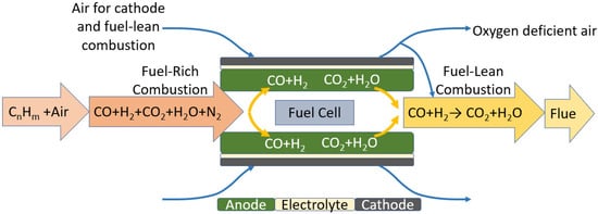
Figure 1.
Schematic of the tubular FFC showing the different reaction zones.
A mixture of a hydrocarbon fuel and air is sent to the fuel-rich combustion chamber. The fuel/air composition going to the fuel-rich combustion chamber is characterized in terms of equivalence ratio (Φ), as shown in Equation (1). Φ is the ratio of the fuel/air ratio (nfuel/nair) of the gas composition to the fuel/air ratio of the mixture at stoichiometry (nSfuel/nSair). Thus Φ > 1 represents fuel-rich combustion and Φ < 1 represents fuel-lean combustion, whereas Φ = 1 represents combustion at stoichiometric conditions.
The SOFC in the FFC setup consists of porous electrodes and a dense electrolyte layer sandwiched between the cathode and the anode. Nickel is commonly used as the anode material, and LSCF (LaxSr1−xCoyFe1−yO3) is commonly used as the cathode material [38,39]. The electrodes have high electronic and ionic conductivity, whereas the electrolyte has high ionic but ideally no electronic conductivity to prevent an internal short circuit [40]. Thus, materials like Yttria Stabilized Zirconia (YSZ) and Samaria Doped Ceria (SDC) are used to make the electrolyte, as they have high O2- ion conductivity at the target temperature (~1073 K).
In the next few sections, the operating principles of the fuel-rich combustion, the SOFC, and the fuel-lean combustion are outlined. In this paper, modeling efforts mainly focus on the SOFC, since the fuel-rich and fuel-lean combustion models are well established in the literature and are largely independent of the fuel cell. More details of fuel-rich and fuel-lean combustion models can be found in a previous study [37].
2.2. Fuel-Rich Combustion
Fuel-rich combustion in the FFC setup performs the function of a typical fuel-reformer, such as a steam or water gas shift reactor used for DC-SOFC. This is the first step of the FFC operation, and it is responsible for generating syngas for the fuel cell to electrochemically oxidize. A fuel-rich mixture of a hydrocarbon fuel (e.g., CH4) is sent to the fuel-rich combustion chamber, where partial oxidation of the fuel forms syngas (CO+H2) and smaller quantities of CO2 and H2O, as shown in Equation (2). In Equation (2), a–e are the mole fractions of the respective species in the fuel-rich combustion exhaust.
The element balance for the fuel-rich combustion reaction is dependent on Φ, as shown in Equations (3)–(6).
C: a + c = Φ
H: 2b + 2d = 4 Φ
O: a + 2c + d = 4
N: e = 7.52
The total enthalpy released in the fuel-rich combustion reaction (ΔHRC) can be calculated using the molar flow rate () for each species and the molar specific enthalpy for each species. In Equation (7), Tin,RC and Tout,RC are the temperatures of the species at the inlet and outlet of the fuel-rich combustion chamber.
Fuel-rich combustion increases the temperature of the products, allowing the fuel cell to operate at the target temperature (~1073 K). A common method of simulating the fuel-rich combustion exhaust uses chemical equilibrium to estimate the composition at operating conditions [41]. Programs such as NASA Chemical Equilibrium and Applications (NASA CEA) are typically used for this purpose. The software approximates the products at equilibrium by minimizing the Gibbs’ free energy of the composition at a given Φ and temperature for one mole exhaust [41]. NASA CEA provides a good approximation of the fuel-rich combustion exhaust and has been used in previous FFC literature [22]. Thus, NASA CEA software can be used to obtain the values of a–e in Equation (2) for one mole of fuel after fuel-rich combustion.
2.3. Fuel Cell
2.3.1. Fuel Cell Potential
The exhaust from the fuel-rich combustion passes through the fuel cell to generate heat and electricity. Only the CO and H2 from the fuel-rich exhaust are used as fuel. The electrochemical reactions of CO and H2 that occur at the boundary of the anode and electrolyte are shown in Equations (8) and (9).
The overall fuel cell reaction, including all the products of combustion in the exhaust, thus follows, as shown in Equation (10).
Considering only the species taking part in the electrochemical reaction and dividing Equation (10) by the total moles of syngas (a+b) leads to Equation (11).
Note that one mole of syngas uses 1/2 mole of O2 at stoichiometry. Due to this, the coefficient of O2 in Equation (2) is .
2.3.2. Standard State Thermoneutral Potential
Equations (10) and (11) are used to calculate the thermodynamic potential of the fuel cell. First, the standard state (298 K and 1 atm) thermal neutral potential (Eth) is calculated using the molar specific enthalpy change (Δh0FC) in the fuel cell reaction and the coefficients of species in Equation (11). This is shown in Equation (12), where h0i are the molar specific enthalpies of species ‘i’ at the operating temperature.
From Equation (12), the Eth follows as shown in Equation (13), where ne is the number of electrons exchanged in the reaction (i.e., 2 per mole of syngas) and F is Faraday’s constant.
2.3.3. Standard State Reversible Potential
The reversible cell potential at reaction temperature (Erev) is the theoretically predicted thermodynamic potential of the fuel cell at the fuel cell temperature. Erev contains two main parts under constant pressure conditions, as shown in Equation (14). In Equation (14), E0rev is the reversible potential at the operating temperature of the fuel cell, and EC is the concentration correction factor.
The Erev of the fuel cell for reaction in Equation (10) is calculated similar to Eth but uses the molar specific Gibbs’ free energy of the species involved (gi) instead of hi. Thus, the total molar specific Gibbs’ energy change in the fuel cell is given by Equation (15).
Thus, Erev of the fuel cell is given by Equation (16).
EC arises from dilution of the fuel with inert or unreactive species. EC is calculated as shown in Equation (17).
In Equation (17), R is the universal gas constant, and K is the equilibrium constant of the fuel cell reaction. K for the reaction in Equation (11) is calculated as shown in Equation (18), where [i] is the concentration of the species ‘i’. The model only uses the species taking part in the fuel cell reaction (CO, H2, O2) for the calculation of K.
In Equation (18), [i] is the coefficient of the species ‘i’ in Equation (10) if the coefficient is also the mole fraction of each species. Thus, Equation (18) can be converted to Equation (19), assuming the O2 concentration in air as 21%.
Experimentally, Erev remains close to the experimental value of the open circuit voltage (OCV). Irreversibilities in the fuel cell at equilibrium lead to small deviations from the theoretical value.
2.4. Fuel Cell Kinetic Losses
When current is generated in the fuel cell, several losses or overpotentials (ɳ) occur, causing a drop in the fuel cell potential. The three main losses in the fuel cell are activation loss, ohmic loss, and concentration loss. Each of these losses are discussed in the following sections.
2.4.1. Activation Loss
When current starts flowing from the fuel cell, a portion of the cell overpotential is provided for overcoming the activation barriers of the fuel oxidation and oxygen reduction reactions. This leads to a loss of the cell potential, called activation loss (ɳact). ɳact is calculated using the Tafel equation [10], as shown in Equation (20). In Equation (20), α is the charge transfer coefficient, j0 is the exchange current density of the reaction, and j is the actual current density of the reaction.
As the Tafel equation works well only for j > 4j0, this method provides large errors for j < 4j0 and is negative for j < j0. Thus, instead of Equation (20), an approximation of Equation (20) with inverse hyperbolic sine is used to calculate activation loss at all current densities, as shown in Equation (21) [33].
where j0 is the current density that exists when the forward and reverse reaction rates are equal, i.e., at equilibrium. j0 results from the equal number of oxidation and reduction reactions, with no current actively being extracted from the fuel cell. j0 can be experimentally calculated as the x-intercept of the Tafel equation.
Activation losses also depend upon α, the charge transfer coefficient. α is a kinetic parameter that determines the symmetry of the activation barrier and always ranges from 0 to 1 [10]. This parameter determines how the electrical potential changes the sizes of the oxidation and reduction activation barriers. α varies linearly with the parameter (1-α with ), where Ia is the partial anodic current [35].
2.4.2. Ohmic Loss
Ohmic loss occurs due to resistance to the motion of electrons and ions by electrode and electrolyte materials. Most fuel cells operate in the ohmic region where the concentration losses are near minimum. The ohmic loss (ɳohm) is calculated using Ohm’s law, as shown in Equation (22) [10].
In Equation (22), rhok is the temperature-dependent electrical resistivity (or ionic resistivity for electrolyte) of the material, AFC is the active area of the fuel cell (connected to current collector), and δk is the thickness of the respective layer ‘k’ (k = anode, cathode, electrolyte). Generally, in anode-supported fuel cells (like the one used in this study), anode resistance is significantly higher than the cathode or electrolyte due to its much larger thickness compared to the cathode and electrolyte.
2.4.3. Concentration Loss
The concentration loss (ɳconc) arises from the finite rate of mass transport of the fuel and oxidant. At high current densities, the given flow rate of the species cannot match the increased fuel consumption rate. This causes large kinetic losses and a decrease in the cell potential. ɳconc can be calculated as shown in Equation (23).
In Equation (23), is the limiting current density of the fuel cell. Assuming the concentration of reactants at the activation sites (CR,0) to be constant, according to Fick’s law, in the Nernst diffusion layer, jL can be calculated as shown in Equation (24), where ε is the porosity and τ is the tortuosity of the anode.
In Equation (24), Df is the effective self-diffusivity of the fuel, and δ is the thickness of the Nernst diffusion layer. For simplicity, CR,0 is assumed to be equal to the bulk channel reactant concentration.
In calculating Df, the first step is the binary diffusivity of each pair of gases in the incoming mixture, using the kinetic theory of gases as shown in Equation (25) [10].
In Equation (25), a = 3.640 × 10⁻⁴ and b = 2.334 if the pair ij contains polar molecules, and a = 2.745 × 10⁻⁴ and b = 2.334 if the pair contains non-polar molecules only. TC is the critical temperature, pC is the critical pressure, p is the total operating pressure, and M is the molecular weight of species i and j, respectively. The self-diffusion coefficient of species ‘i’ in a multicomponent system (e.g., CO+H2+CO2+H2O) is calculated using the Maxwell–Stefan equation, as shown in Equation (26) [28,42].
In Equation (26), is the self-diffusivity and X is the mole fraction of the respective species. Thus, from Equations (25) and (26), the self-diffusivity of the specific fuel mixture containing CO and H2 can be calculated as shown in Equation (27).
The Nernst diffusion layer is a virtual layer within which the gradient of ion concentration is constant and equal to the true gradient at the electrode–electrolyte interface. The thickness of this diffusion layer (δ) depends on the diffusivity of reactants [36], which, as established by Equation (24), depends on the reactant concentration. With an O2− conducting electrolyte, this diffusion layer is present at the boundary of the anode and electrolyte. This model assumes no change in the fuel concentration from the bulk channel concentration to the anode-diffusion layer boundary.
The operating voltage of the fuel cell at an arbitrary current density j (Ej) is thus given by Equation (28). Equation (28) represents the main governing equation of the proposed parametric SOFC model.
Since the values of α and δ are not calculated theoretically, the parametric model (30), parameterized in α and δ, is used to fit the experimental polarization curves, as shown in Equation (29), where jL is a function of δ.
Fitting Equation (29) to the experimental polarization curves can provide values of α and δ. Consequently, the operating power density of the fuel cell at an arbitrary current density j (PDj) is given by Equation (30).
2.5. Fuel Cell Efficiencies
Due to various losses and kinetic limitations in the fuel cell, not all fuel that is supplied to the fuel cell will participate in the electrochemical reaction. Of the fuel that actually participates in the electrochemical reaction, the fuel cell converts the available chemical energy into heat and electricity. The fuel utilization efficiency (εFU) and fuel cell efficiency (εFC) help characterize these conversions.
2.5.1. Fuel Utilization Efficiency
The total current density (jmax) available in the incoming fuel can be calculated as shown in Equation (31). In Equation (31), AFC is the active area of the fuel cell, and is the molar flow rate of fuel supplied to the fuel cell.
εFU results from all the kinetic losses of the fuel cell. The limitations of fuel cell kinetics result in a reduction of the total fuel oxidized compared to the total fuel available in the bulk flow stream. εFU is defined as the ratio of the actual current density (j) generated by the fuel cell to the total available current density that could be generated by the fuel mixture if all the fuel oxidizes (jmax). The εFU at any voltage (εFU,V) is defined in Equation (32), where jV is the current density measured at that voltage.
2.5.2. Fuel Cell Efficiency
εFC results from the inability of the fuel cell to convert all the fuels’ chemical energy into electrical power. It is defined as the ratio of the total electrical power produced in the fuel cell to the total chemical energy available in the utilized fuel. In Equation (33), Δhf is the mole specific enthalpy of the fuel.
2.6. Fuel-Lean Combustion
Unreacted fuel from the fuel cell is combusted in an excess oxygen (fuel-lean) environment to generate heat to maintain the fuel cell temperature. The total heat generated in the fuel-lean combustion is shown in Equation (34), where represents the remaining moles of the reactant species after the fuel cell reaction, and Tin/out,LC represents the inlet and outlet temperatures of the species, respectively.
3. Experimental Setup
Experiments were conducted on a tubular fuel cell and polarization curves under a wide range of FFC operating conditions. Figure 2 shows the schematic of the experimental fuel cell setup. In the experiment, gas compositions containing CO, H2, N2, and CO2 were mixed and sent to a tubular fuel cell placed inside a furnace at 1073 K. Air for oxidation was taken from the environment. The details of the experimental flow rate calculations and the fuel cell details are provided in the following sections.
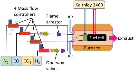
Figure 2.
Schematic of the experimental setup used for understanding the kinetic parameters.
3.1. Species Flow Rate
The experiment was conducted with N2, CO2, H2, and CO2 as the composition of the model dry exhaust of methane partial oxidation in air at 1073 K [43]. The species mole fractions were based on chemical equilibrium calculations from NASA CEA. Along with the model dry exhaust, a few custom compositions were used to understand the impact of the fuel concentration on the FFC operation. The fuel compositions used in the FFC experiment and their respective identifiers are shown in Table 1.

Table 1.
Mole fractions of the gas species used in the experiment.
In Table 1, the gas compositions are chosen to include a wide variety of different fuel concentrations that can be present in the FFC. CH2 and CCO were chosen to isolate the effects of the fuel (i.e., CO and H2) from CO2. Since the fuel cell operates under model dry exhaust, XN2 is the sum of both XH2O and XN2 from the NASA CEA predictions to maintain the level of fuel dilution. The experiment was conducted under a constant fuel-rich exhaust flow rate of 150 sccm at 298 K and 1 atm. The volumetric flow rate of species ‘i’ is thus the product of the total flow rate and Xi. To meter the gas flows, mass flow controllers were used.
3.2. Measurement Techniques
The model dry exhaust gases were mixed and sent to the fuel cell placed inside a furnace at 1073 K. The current density and the voltage were measured using a sourcemeter (Keithley 2460) connected to both the cathode and anode via current collectors using the four-probe technique. In the four-probe technique, a high impedance current source supplies current through two outer probes, while a voltmeter measures the voltage across the two inner probes [43]. Flame arrestors were placed in line with the CO and H2 lines to avoid flashback. Air for oxidation came from the environment, as shown in Figure 2.
3.3. Fuel Cell Fabrication
The details of the fabrication technique for fuel cell anode, NiO + YSZ ((Y2O3)0.08(ZrO2)0.92), and electrolyte, YSZ, were reported previously in the literature [14]. The anode was pre-fired at 1373 K. The electrolyte was dip-coated on the anode and sintered, with a final thickness of ~22 µm. The final inner and outer diameter of the tubular fuel cell was 2.2 mm and 3.3 mm, respectively. A buffer layer of Sm0.20Ce0.80O2−x (SDC) was sprayed onto the electrolyte to prevent adverse reactions between the cathode and electrolyte. The fuel cell was then dried and sintered at 1673 K for 4 h. A cathode made of SDC + LSCF (La0.60Sr0.40)0.95Co0.20Fe0.80O3-x) was dip-coated onto the buffer layer, dried, and sintered at 1373 K for 2 h. A silver wire and silver paste were used as a current collector on the cathode and anode. The total active cell area after these modifications was 4.14 cm2. The porosity (ε) of the fuel cell anode measured using scanning electron microscopy (SEM) was 6.34%. The τ of the SOFC Ni-YSZ anode was taken as 2 from the literature [44].
3.4. Experimental Error and Reproducibility
The main experimental parameters include voltage, current, and flowrate measurements. A Keithley 2460 sourcemeter has a maximum error of ±5.58 mA or ±1.33 mA/cm2 for the current source at the maximum current (~900 mA/cm2). For the voltage source, the maximum error is ±0.00165 V or 0.165% at the maximum voltage of around 1 V. A bubble-meter was used to verify the factory-calibrated flow meters, and the error was found to be within ±3% of the species flow rates. Since these errors are small, previously published results have not displayed them on j-V curves of the fuel cell. In regard to reproducibility, all polarization curves were measured five different times, with comparable results across all measurements. Factory-calibrated flow meters were used in the recommended ranges of the flow rates. The calibration was further verified multiple times.
4. Results and Discussion
This section starts with a comparison of experimental and model-predicted polarization curves for the fuel cell. The polarization curves are then broken down into several relevant kinetic factors. The dependence of the kinetic factors with the composition of inlet gas is then used to draw conclusions about the effect of gas composition on the FFC performance. Figure 3 shows the experimental data and model-predicted polarization curves for different gas compositions. The model is able to predict the experimental results to a high degree of accuracy (>95%) at all values of j. The experiment is terminated at V ~ 0.1 V to prevent anode reoxidation. The j at the termination of the experiment is termed jT. In the experiment, the fuel cell had a lower jT for the CH2 than the CCO fuel composition. Since CO and H2 represent the fuel in the FFC gas composition, we define CR,0 = XCO + XH2, which increases from the lowest concentration (for CH2 and CCO, CR,0 = 0.1) to the highest concentration (for Φ = 3, CR,0 = 0.48) tested in these experiments.
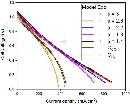
Figure 3.
Experimental and model-predicted polarization curves for different gas compositions.
Figure 3 shows that jT increases with CR,0. The slope of the curves at low j values is almost equal, indicating that ɳohm varies linearly with j and does not change with CR,0. ɳohm only depends on rhok, which is a function of TFC (which is constant at 1073 K) and does not depend on CR,0. The next few sections discuss several factors that contribute to the results in Figure 3.
4.1. Dependence of Cell Potentials on Fuel Concentration
Figure 4 shows the variation of experimental open circuit voltage (OCV) and Erev with CR,0. The results show that Erev is able to approximate the OCV well. After the initial dip at Φ = 1.4, Erev increases with an increase in CR,0. The results confirm that addition of CO2 at Φ = 1.4 decreases Erev compared to lower concentrations. As Φ increases above 1.4, an increase in fuel concentration and decrease in CO2 concentration leads to an increase in Erev.
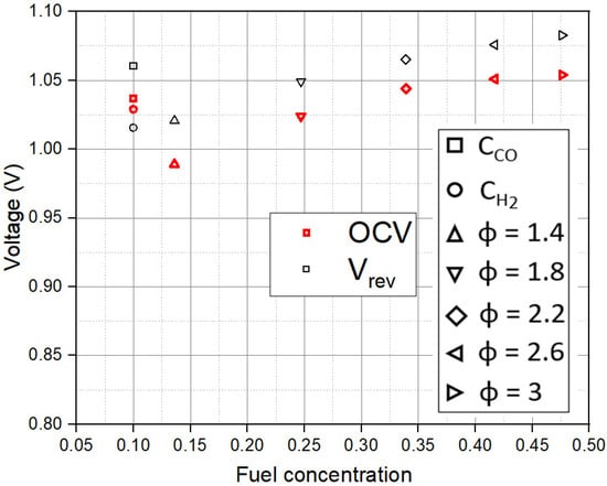
Figure 4.
Dependence of the open circuit voltage (OCV) and reversible potential (Vrev) on fuel concentration (CR,0).
4.2. Dependence of Activation Losses on Fuel Concentration
Figure 5 shows the dependence of ɳact on j at different CR,0. Figure 5 shows that for low values of CR,0 (up to Φ = 1.4) ɳact is constant and low at the same j values. This happens because at low CR,0, the available reaction sites in the fuel cell can activate most of the available fuel in the gas composition. As CR,0 increases, the limited number of reaction sites cannot accommodate the arbitrarily increasing fuel CR,0 in the limited residence time in the fuel cell. The fuel cell thus has a larger ɳact. ɳact depends on the number of reaction sites, which vary with porosity, tortuosity, surface roughness, dimensions of the fuel cell, etc. [10]. Thus, modifying any of these parameters should theoretically affect ɳact. More experimental work in FFCs is required to confirm this hypothesis. Thus, care needs to be taken while designing the FFC to account for the range of CR,0 that the FFC is expected to operate under and to minimize the effect of activation limitations. When the jT is-limited by high ɳact, the fuel cell is considered activation-limited.
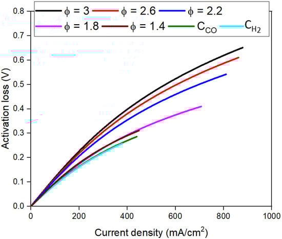
Figure 5.
Dependence of activation loss (ɳact) on current density (j) for different fuel concentrations.
4.3. Dependence of Concentration Loss on Fuel Concentration
Figure 6 shows the dependence of ɳconc on j at various values of CR,0. ɳconc decreases for similar j values with an increase in CR,0. Since H2 electrochemically oxidizes much faster than CO, as observed in the literature [45], ɳconc is much higher for CH2 than CCO. As CR,0 increases, a smaller portion of the overpotential is needed to overcome the mass transfer losses due to available excess inactivated fuel. This reduction in ɳconc thus does not lead to a significant rise in the jT and does not indicate improvement in fuel cell kinetics. A decrease in ɳconc increases the fuel cell current density only if a large number of reaction sites are available to activate a significant portion of available fuel, i.e., ɳact is low. When the jT is limited by high ɳconc, the fuel cell is considered concentration-limited.
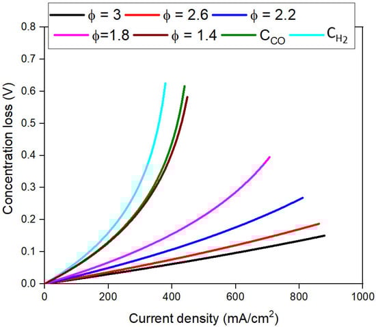
Figure 6.
Dependence of concentration loss (ɳconc) on current density (j) at different fuel concentrations.
4.4. Dependence of Fuel Utilization Efficiency on Fuel Concentration
εFU is calculated at the termination of the experiment to observe the effect of all the fuel cell losses. Figure 7 shows that εFU decreases with an increase in CR,0. The εFU of CCO is higher than CH2 because CH2 experiences larger ɳconc than CCO, as described earlier. Observing the trends in ɳact and ɳconc, at low CR,0 up to Φ = 1.4, εFU is limited by ɳconc (concentration limited), and beyond Φ = 1.4, εFU is limited by ɳact (activation limited). This difference is also apparent in Figure 3, where for CR,0 up to Φ = 1.4, a rapid drop in j at low voltages indicates high ɳconc. The drop in j with V at low voltages in Figure 3 is much more gradual for Φ ≥ 1.8. The results suggest that the optimum value of CR,0, where the activation limitations and concentration limitations are simultaneously low, lies between Φ = 1.4 and Φ = 1.8 for this experimental fuel cell.
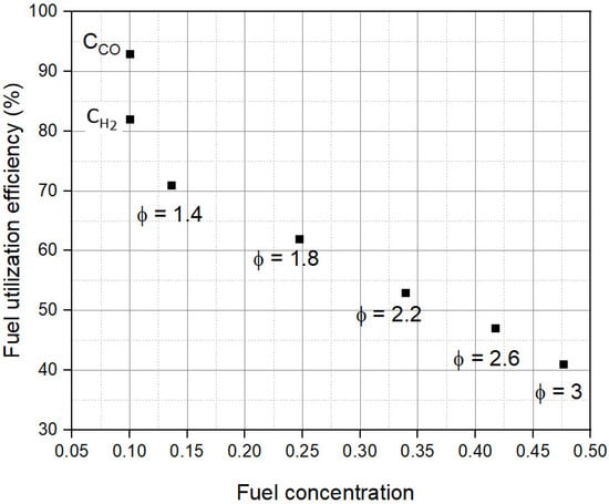
Figure 7.
Dependence of fuel utilization efficiency (εFU) on fuel concentration (CR,0).
4.5. Dependence of Exchange Current Density on Fuel Concentration
Figure 8 shows the variation of j0 with CR,0. The values of j0 shown in Figure 8 are calculated using the x-intercept of the Tafel plot, as described in earlier sections. Since j0 depends on the CR,0, as the CR,0 increases, j0 increases because more total fuel is available in the gas composition. Though j0 is inversely related to ɳact, this increase in j0 does little to reduce the ɳact at higher j values as CR,0 increases. Thus, an increase in j0 is not a sufficient indicator of the improvement in fuel cell activation kinetics.
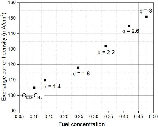
Figure 8.
Dependence of exchange current density (j0) on fuel concentration (CR,0).
4.6. Dependence of Charge Transfer Coefficient on Fuel Concentration
Figure 9 shows the dependence of α on CR,0. As shown, α is much smaller compared to the normally assumed value of 0.5 for all values of CR,0. This indicates the syngas oxidation reaction is not symmetric and favors the reduction reaction in FFCs. Under concentration-limited conditions, α remains constant at ~0.24. This is the primary reason for the similar ɳact for CH2, CCO, and Φ = 1.4 shown in Figure 5.
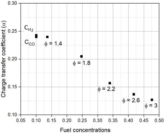
Figure 9.
Dependence of charge transfer coefficient (α) on fuel concentration (CR,0).
As CR,0 further increases, the activation limitations set in and lead to a rapid drop in α with CR,0. This decrease in α indicates worsening activation kinetics and leads to a rapid rise in ɳact and a decrease in εFU at higher CR,0. The results thus suggest that strategies to reduce ɳact will increase α, thereby improving fuel cell kinetics.
4.7. Dependence of Nernst Diffusion Layer Thickness on Fuel Concentration
Figure 10 shows the dependence of δ on CR,0. First, the model results show that δ is much smaller than the thickness of the anode (~400 µm). Under concentration-limited conditions, δ remains constant at ~10 µm. Under activation-limited conditions, δ increases to ~17.5 µm. This variation in δ indicates reaction kinetics differ significantly between concentration-limited and activation-limited conditions. Slower reactions at higher CR,0 values create larger diffusion layers, which rapidly reduces εFU.
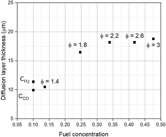
Figure 10.
Dependence of Nernst diffusion layer thickness (δ) on fuel concentration (CR,0).
4.8. Model Sensitivity
Since these results are based on fitted parameters, it is important to check the sensitivity of the model to α and δ. A high parameter sensitivity is better for ensuring that no other value of α and δ also match the experiment, potentially causing conflicting results. Figure 11 shows that the model is sensitive to change in the values of these parameters. As an example, we consider the case of Φ = 2.2. Figure 11 shows the variation of the j-V curves at a constant δ of 18.2 µm but varying α. The cell voltage at j > 0 increases with an increase in α due to reduction in ɳact. As only one value of α (0.157) over a wide range (0.1 < α < 0.3) matches the experimental curve, the results provide confidence in the model.
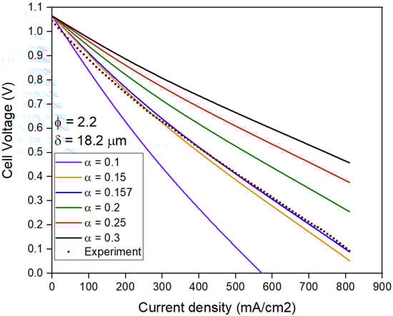
Figure 11.
Polarization curves for Φ = 2.2 with varying charge transfer coefficient (α) and constant Nernst diffusion layer thickness (δ).
Similar to α, the model is very sensitive to δ, as can be seen in Figure 12. The cell voltage at j > 0 decreases with an increase in δ due to an increase in ɳconc. Only δ = 18.2 µm correctly matches the experimental result.
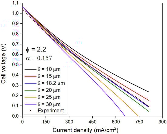
Figure 12.
Polarization curves for Φ = 2.2 with varying Nernst diffusion layer thickness (δ) and constant charge transfer coefficient (α).
5. Conclusions
A model for describing the FFC operation at different fuel concentrations is provided in this paper. The model is parametrized in α and δ and then empirically fitted to the experimental SOFC polarization curves. The model fitted experimental results to >95% accuracy at all values of current density. The results show α is much lower than the normally assumed value of 0.5, indicating asymmetric syngas reaction kinetics, and δ is much smaller than the anode thickness. The high εFU (>70%) at lower fuel concentration values (CR,0) up to Φ = 1.4 is mainly a result of low activation losses, where the FFC current density is mainly concentration-limited. The εFU at higher Φ decreases rapidly with CR,0 due to the onset of activation limitations, which prevents activation of a large portion of the fuel in the limited residence time. Activation-limited fuel cells thus have a much lower εFU than concentration-limited fuel cells. Thus, the model suggests that increasing the number of activation sites should decrease the activation losses and should lead to an increase in fuel utilization and power density under similar current densities. These experiments thus indicate future directions for further validating this model. The charge transfer coefficient is almost constant at ~0.24 for concentration-limited conditions and decreases with CR,0 at the onset of activation limitations. The value of δ remains constant at ~10 µm for concentration-limited conditions and increases to ~17.5 µm under activation-limited conditions, indicating worsening of reaction kinetics under activation-limited conditions. Care should be taken to operate FFC under fuel concentrations where activation and concentration losses are simultaneously low. The results indicate that such a point lies between Φ = 1.4 and Φ = 1.8 for the experimental fuel cell under the given operating conditions.
Author Contributions
Conceptualization, R.G. and R.J.M.; data curation, R.G.; formal analysis, R.G.; funding acquisition, R.J.M.; investigation, R.G.; methodology, R.G. and R.J.M.; project administration, R.J.M.; resources, R.J.M.; software, R.G.; supervision, R.J.M.; validation, R.J.M.; visualization, R.G.; writing—original draft, R.G.; writing—review and editing, R.G. and R.J.M. All authors have read and agreed to the published version of the manuscript.
Funding
This research received no external funding.
Institutional Review Board Statement
Not applicable.
Informed Consent Statement
Not applicable.
Data Availability Statement
The data presented in this study are available in the article.
Conflicts of Interest
The authors declare no conflict of interest.
References
- Ormerod, R.M. Solid Oxide Fuel Cells. Chem. Soc. Rev. 2003, 32, 17–28. [Google Scholar] [CrossRef] [PubMed]
- Al-Khori, K.; Bicer, Y.; Koç, M. Integration of Solid Oxide Fuel Cells into Oil and Gas Operations: Needs, Opportunities, and Challenges. J. Clean. Prod. 2020, 245, 118924. [Google Scholar] [CrossRef]
- Baldi, F.; Moret, S.; Tammi, K.; Maréchal, F. The Role of Solid Oxide Fuel Cells in Future Ship Energy Systems. Energy 2020, 194, 116811. [Google Scholar] [CrossRef]
- Shao, Z.; Haile, S.M.; Ahn, J.; Ronney, P.D.; Zhan, Z.; Barnett, S.A. A Thermally Self-Sustained Micro Solid-Oxide Fuel-Cell Stack with High Power Density. Nature 2005, 435, 795–798. [Google Scholar] [CrossRef] [PubMed] [Green Version]
- Milcarek, R.J.; Garrett, M.J.; Welles, T.S.; Ahn, J. Performance Investigation of a Micro-Tubular Flame-Assisted Fuel Cell Stack with 3000 Rapid Thermal Cycles. J. Power Sources 2018, 394, 86–93. [Google Scholar] [CrossRef]
- Horiuchi, M.; Suganuma, S.; Watanabe, M. Electrochemical Power Generation Directly from Combustion Flame of Gases, Liquids, and Solids. J. Electrochem. Soc. 2004, 151, A1402. [Google Scholar] [CrossRef]
- Vogler, M.; Horiuchi, M.; Bessler, W.G. Modeling, Simulation and Optimization of a No-Chamber Solid Oxide Fuel Cell Operated with a Flat-Flame Burner. J. Power Sources 2010, 195, 7067–7077. [Google Scholar] [CrossRef]
- Kronemayer, H.; Barzan, D.; Horiuchi, M.; Suganuma, S.; Tokutake, Y.; Schulz, C.; Bessler, W.G. A Direct-Flame Solid Oxide Fuel Cell (DFFC) Operated on Methane, Propane, and Butane. J. Power Sources 2007, 166, 120–126. [Google Scholar] [CrossRef]
- Vogler, M.; Barzan, D.; Kronemayer, H.; Schulz, C.; Horiuchi, M.; Suganuma, S.; Tokutake, Y.; Warnatz, J.; Bessler, W.G. Direct-Flame Solid-Oxide Fuel Cell (DFFC): A Thermally Self-Sustained, Air Self- Breathing, Hydrocarbon-Operated SOFC System in a Simple, No-Chamber Setup. ECS Trans. 2007, 7, 555–564. [Google Scholar] [CrossRef]
- O’Hayre, R.; Cha, S.-W.; Colella, W.; Prinz, F.B. Fuel Cell Fundamentals. Intergovernmental Panel on Climate Change, Ed.; John Wiley & Sons, Inc.: Hoboken, NJ, USA, 2016; ISBN 9781119191766. [Google Scholar]
- Endo, S.; Nakamura, Y. Power Generation Properties of Direct Flame Fuel Cell (DFFC). J. Phys. Conf. Ser. 2014, 557, 012119. [Google Scholar] [CrossRef] [Green Version]
- Nakamura, Y.; Endo, S. Power Generation Performance of Direct Flame Fuel Cell (DFFC) Impinged by Small Jet Flames. J. Micromech. Microeng. 2015, 25, 104015. [Google Scholar] [CrossRef]
- Wang, Y.; Sun, L.; Luo, L.; Wu, Y.; Liu, L.; Shi, J. The Study of Portable Direct-Flame Solid Oxide Fuel Cell (DF-SOFC) Stack with Butane Fuel. J. Fuel Chem. Technol. 2014, 42, 1135–1139. [Google Scholar] [CrossRef]
- Hirasawa, T.; Kato, S. A Study on Energy Conversion Efficiency of Direct Flame Fuel Cell Supported by Clustered Diffusion Microflames. J. Phys. Conf. Ser. 2014, 557, 012120. [Google Scholar] [CrossRef] [Green Version]
- Wang, Y.; Shi, Y.; Yu, X.; Cai, N.; Qian, J.; Wang, S. Experimental Characterization of a Direct Methane Flame Solid Oxide Fuel Cell Power Generation Unit. J. Electrochem. Soc. 2014, 161, F1348–F1353. [Google Scholar] [CrossRef]
- Zhu, X.; Lü, Z.; Wei, B.; Huang, X.; Wang, Z.; Su, W. Direct Flame SOFCs with La0.75Sr0.25Cr0.5Mn0.5O3−δ∕Ni Coimpregnated Yttria-Stabilized Zirconia Anodes Operated on Liquefied Petroleum Gas Flame. J. Electrochem. Soc. 2010, 157, B1838. [Google Scholar] [CrossRef]
- Wang, Y.; Shi, Y.; Cao, T.; Zeng, H.; Cai, N.; Ye, X.; Wang, S. A Flame Fuel Cell Stack Powered by a Porous Media Combustor. Int. J. Hydrogen Energy 2018, 43, 22595–22603. [Google Scholar] [CrossRef]
- Wang, Y.; Zeng, H.; Shi, Y.; Cao, T.; Cai, N.; Ye, X.; Wang, S. Power and Heat Co-Generation by Micro-Tubular Flame Fuel Cell on a Porous Media Burner. Energy 2016, 109, 117–123. [Google Scholar] [CrossRef]
- Milcarek, R.J.; Garrett, M.J.; Wang, K.; Ahn, J. Micro-Tubular Flame-Assisted Fuel Cells Running Methane. Int. J. Hydrogen Energy 2016, 41, 20670–20679. [Google Scholar] [CrossRef] [Green Version]
- Wang, K.; Zeng, P.; Ahn, J. High Performance Direct Flame Fuel Cell Using a Propane Flame. Proc. Combust. Inst. 2011, 33, 3431–3437. [Google Scholar] [CrossRef]
- Hossain, M.M.; Myung, J.; Lan, R.; Cassidy, M.; Burns, I.; Tao, S.; Irvine, J.T.S. Study on Direct Flame Solid Oxide Fuel Cell Using Flat Burner and Ethylene Flame. ECS Trans. 2015, 68, 1989–1999. [Google Scholar] [CrossRef] [Green Version]
- Milcarek, R.J.; Garrett, M.J.; Baskaran, A.; Ahn, J. Combustion Characterization and Model Fuel Development for Micro-Tubular Flame-Assisted Fuel Cells. J. Vis. Exp. 2016, e54638. [Google Scholar] [CrossRef] [PubMed]
- Wang, Y.; Zeng, H.; Cao, T.; Shi, Y.; Cai, N.; Ye, X.; Wang, S. Start-up and Operation Characteristics of a Flame Fuel Cell Unit. Appl. Energy 2016, 178, 415–421. [Google Scholar] [CrossRef]
- Milcarek, R.J.; Ahn, J. Rich-Burn, Flame-Assisted Fuel Cell, Quick-Mix, Lean-Burn (RFQL) Combustor and Power Generation. J. Power Sources 2018, 381, 18–25. [Google Scholar] [CrossRef]
- Milcarek, R.J.; Ahn, J.; Zhang, J. Review and Analysis of Fuel Cell-Based, Micro-Cogeneration for Residential Applications: Current State and Future Opportunities. Sci. Technol. Built Environ. 2017, 23, 1224–1243. [Google Scholar] [CrossRef]
- Ghotkar, R.; Milcarek, R.J. Investigation of Flame-Assisted Fuel Cells Integrated with an Auxiliary Power Unit Gas Turbine. Energy 2020, 204, 117979. [Google Scholar] [CrossRef]
- Kakaç, S.; Pramuanjaroenkij, A.; Zhou, X.Y. A Review of Numerical Modeling of Solid Oxide Fuel Cells. Int. J. Hydrog. Energy 2007, 32, 761–786. [Google Scholar] [CrossRef]
- Hajimolana, S.A.; Hussain, M.A.; Daud, W.M.A.W.; Soroush, M.; Shamiri, A. Mathematical Modeling of Solid Oxide Fuel Cells: A Review. Renew. Sustain. Energy Rev. 2011, 15, 1893–1917. [Google Scholar] [CrossRef]
- Brandon, N. Solid Oxide Fuel Cell Lifetime and Reliability: Critical Challenges in Fuel Cells; Elsevier Science: Amsterdam, The Netherlands, 2017; ISBN 9780128097243. [Google Scholar]
- Costamagna, P. Modeling of Solid Oxide Heat Exchanger Integrated Stacks and Simulation at High Fuel Utilization. J. Electrochem. Soc. 2006, 145, 3995. [Google Scholar] [CrossRef]
- Shin, D.; Nam, J.H. An Effectiveness Model for Electrochemical Reactions in Electrodes of Intermediate-Temperature Solid Oxide Fuel Cells. Electrochim. Acta 2015, 171, 1–6. [Google Scholar] [CrossRef]
- Yakabe, H.; Hishinuma, M.; Uratani, M.; Matsuzaki, Y.; Yasuda, I. Evaluation and Modeling of Performance of Anode-Supported Solid Oxide Fuel Cell. J. Power Sources 2000, 86, 423–431. [Google Scholar] [CrossRef]
- Gebregergis, A.; Pillay, P.; Bhattacharyya, D.; Rengaswemy, R. Solid Oxide Fuel Cell Modeling. IEEE Trans. Ind. Electron. 2009, 56, 139–148. [Google Scholar] [CrossRef] [Green Version]
- Chan, S.H.; Khor, K.A.; Xia, Z.T. Complete Polarization Model of a Solid Oxide Fuel Cell and Its Sensitivity to the Change of Cell Component Thickness. J. Power Sources 2001, 93, 130–140. [Google Scholar] [CrossRef]
- Guidelli, R.; Compton, R.G.; Feliu, J.M.; Gileadi, E.; Lipkowski, J.; Schmickler, W.; Trasatti, S. Defining the Transfer Coefficient in Electrochemistry: An Assessment (IUPAC Technical Report). Pure Appl. Chem. 2014, 86, 245–258. [Google Scholar] [CrossRef] [Green Version]
- Molina, A.; González, J.; Laborda, E.; Compton, R.G. On the Meaning of the Diffusion Layer Thickness for Slow Electrode Reactions. Phys. Chem. Chem. Phys. 2013, 15, 2381–2388. [Google Scholar] [CrossRef]
- Ghotkar, R.; Milcarek, R.J. Modeling of Micro-Tubular Flame-Assisted Fuel Cells. In Proceedings of the American Society of Mechanical Engineers, Power Division POWER, Salt Lake City, UT, USA, 4 August 2020. [Google Scholar]
- Costa-Nunes, O.; Gorte, R.J.; Vohs, J.M. Comparison of the Performance of Cu-CeO2-YSZ and Ni-YSZ Composite SOFC Anodes with H2, CO, and Syngas. J. Power Sources 2005, 141, 241–249. [Google Scholar] [CrossRef] [Green Version]
- Pihlatie, M.H.; Kaiser, A.; Mogensen, M.; Chen, M. Electrical Conductivity of Ni-YSZ Composites: Degradation Due to Ni Particle Growth. Solid State Ion. 2011, 189, 82–90. [Google Scholar] [CrossRef]
- Ahamer, C.; Opitz, A.K.; Rupp, G.M.; Fleig, J. Revisiting the Temperature Dependent Ionic Conductivity of Yttria Stabilized Zirconia (YSZ). J. Electrochem. Soc. 2017, 164, F790–F803. [Google Scholar] [CrossRef]
- McBride, B.J.; Gordon, S.; McBride, B.J. Computer Program for Calculation of Complex Chemical Equilibrium Compositions and Applications; NASA Lewis Research Center: Cleveland, OH, USA, 1994; pp. 1–175. [Google Scholar]
- Suwanwarangkul, R.; Croiset, E.; Fowler, M.W.; Douglas, P.L.; Entchev, E.; Douglas, M.A. Performance Comparison of Fick’s, Dusty-Gas and Stefan-Maxwell Models to Predict the Concentration Overpotential of a SOFC Anode. J. Power Sources 2003, 122, 9–18. [Google Scholar] [CrossRef]
- Milcarek, R.J.; Wang, K.; Falkenstein-Smith, R.L.; Ahn, J. Micro-Tubular Flame-Assisted Fuel Cells for Micro-Combined Heat and Power Systems. J. Power Sources 2016, 306, 148–151. [Google Scholar] [CrossRef] [Green Version]
- Bao, C.; Jiang, Z.; Zhang, X. Mathematical Modeling of Synthesis Gas Fueled Electrochemistry and Transport Including H2/CO Co-Oxidation and Surface Diffusion in Solid Oxide Fuel Cell. J. Power Sources 2015, 294, 317–332. [Google Scholar] [CrossRef]
- Yao, W. Hydrogen and Carbon Monoxide Electrochemical Oxidation Reaction Kinetics on Solid Oxide Fuel Cell Anodes. Ph.D. Thesis, University of Waterloo, Waterloo, ON, Canada, 2013. Available online: http://hdl.handle.net/10012/7772 (accessed on 15 January 2022).
Publisher’s Note: MDPI stays neutral with regard to jurisdictional claims in published maps and institutional affiliations. |
© 2022 by the authors. Licensee MDPI, Basel, Switzerland. This article is an open access article distributed under the terms and conditions of the Creative Commons Attribution (CC BY) license (https://creativecommons.org/licenses/by/4.0/).