Abstract
This article presents the selection of location and sizing of multiple distributed generators (DGs) for boosting performance of the radial distribution system in the case of constant power load flow and constant impedance load flow. The consideration of placing and sizing of DGs is to meet the load demand. This article tries to overcome the limitations of existing techniques for determining the appropriate location and size of DGs. The selection of DG location is decided in terms of real power losses, accuracy, and sensitivity. The size of DG is measured in terms of real and reactive power. Both positioning and sizing of DG are analyzed with the genetic algorithm and the heuristic probability distribution method. The results are compared with other existing methods such as ant-lion optimization algorithm, coyote optimizer, modified sine-cosine algorithm, and particle swarm optimization. Further, the power quality improvement of the network is assessed by positioning D-STATCOM, and its location is decided on the basis of the nearby bus having poor voltage profile and high total harmonic distortion (THD). The switching and controlling of D-STATCOM are assessed with fuzzy logic controller (FLC) for improving the performance parameters such as voltage profile and THD at that particular bus. The proposed analytical approach for the system is tested on the IEEE 33 bus system. It is observed that the performance of the system with the genetic algorithm gives a better solution in comparison to heuristic PDF and other existing methods for determining the optimal location and size of DG. The introduction of D-STATCOM into the system with FLC shows better performance in terms of improved voltage profile and THD in comparison to existing techniques.
1. Introduction
The current activities of the advanced power system have become very complicated, which needs to necessarily satisfy the increasing energy needs in an efficient manner [1,2]. The civil, fiscal, and other substantial considerations warrant the site of generation centers being placed at places distant from load centers. The reorganization and deregulation of power companies have led to making system governance unpredictable. The factors which are to be considered while carrying out extension of the transmission system are the following: cutback stability margins, chances of tripping outages, and rising power cuts. The distributed generator (DG) installation would be of the utmost benefit where the installation of new transmission lines and setting up of new power-generating units are not feasible [3,4,5]. It is also reasonable to believe that the selection of the right DG technology, including the optimal location and scale of the DG, would help in decreasing the losses in such a system. The purpose of optimally placing DG in a power system network is for achieving correct operation of the network with system error minimization and voltage profile enhancement inclusive of improved stability, reliability, and load ability [6,7]. In contrast to the classical approach, smart techniques for optimal DG sizing and positioning are simple and have good convergence characteristics for application to composite power system networks [8,9,10]. DG is also capable of significantly mitigating harmonics and improving the voltage profile along with acquiesced transmission and distribution investment [11,12,13]. DG is flexible enough to locate anywhere in the system as per requirement of minimum transmission losses [14,15,16]. There have been many techniques proposed to perform such activities as load durability test, exact loss formula, Newton–Raphson, Gauss–Seidal method etc., [17,18,19]. At present, in the era of soft computing technique, every system is trying to obtain fast convergence region so as to reduce the minimum losses with lesser component involved [20,21].
The biggest challenge is to find the optimal size of DG to fulfil the load requirements. It is observed that there are four types of DG given as:
- (a)
- DG1: It supports only real power; no component of reactive power at unity power factor. For example: solar PV array.
- (b)
- DG2: It supports both real power and reactive power at 0.8–0.85 power factor leading. For example: wind, tidal geothermal.
- (c)
- DG3: It supports only reactive power; no component of real power at 0 power factor. For example: synchronous condenser, capacitor bank.
- (d)
- DG4: It absorbs the real power, giving the reactive power to the system at 0.8–0.85 power factor lagging. For example: doubly-fed induction generator [22,23,24].
Recent work has found that there are many advantages to the installation of DGs within the power system; namely raising the efficiency of the output and lowering energy deficit on the electrical grid [25,26,27,28]. In this article, only DG2 is used as per system requirements. The size and location of DG were proposed in many articles by using different techniques such as crow bar search method, neural network, evolutionary algorithm, intelligent water droplet, swarm optimization, etc. [29,30,31,32,33]. The advanced algorithms [34,35] or other existing techniques for identifying the size and location of DG have the biggest challenge of improper total harmonic distortion (THD), sensitivity, and accuracy. It is observed in literature that the THD value obtained was in the range of 15–18%, accuracy and sensitivity are also in the range of 10–15% which are quite high and inadequate, due to which voltage profile is distorted. Such issues with existing techniques create the motivation to overcome these problems. These issues are satisfactorily resolved with the proposed scheme. The genetic algorithm (GA) is proposed to determine the sizing and location of DG with improved THD, accuracy, sensitivity, and voltage profile. GA tends to be more highly permissible than heuristic optimization strategies in order to find the optimal results with less effort than absolute search. In this paper, heuristic optimization strategy which is a combination of two methods, namely, Poisson distribution method and normal distribution method, is also utilized to find the performance of the radial distribution system and show the effectiveness of GA in its comparison. Such a heuristic method requires more effort for providing detailed solutions in terms of accuracy, sensitivity, realism, and power loss. In order to have better results with minimal efforts, GA is applied. It is also observed that the proposed technique gives better results in comparison to existing techniques presented in literature [4,9,12,15,17,20,28,30,32,35,36,37,38,39,40,41,42,43,44,45]. However, to analyze the efficacy of the proposed work in this paper, the results achieved are compared with the existing techniques such as ant-lion optimization algorithm [42], coyote optimizer [43], modified sine-cosine algorithm [44], and particle swarm optimization [45]. The GA seems to have the main advantage of utilizing entity definition, i.e., strings, instead of handling such entities themselves. Multiple problems in electricity grid optimization are manifestations in numerical optimization but linear and other nonlinear methods in programming consider them difficult to address. In this article, the heuristic probability distribution method and GA are applied for finding the best location and sizing of DG in the IEEE 33 bus system for the constant power load model (CPLF) and the constant impedance load model (CILF). The performance parameters show the superiority of GA over the heuristic probability distribution method and other existing methods such as ant-lion optimization algorithm [42], coyote optimizer [43], modified sine-cosine algorithm [44], and particle swarm optimization [45] in the IEEE 33 standard bus system. By considering lower real power losses, improved accuracy, and sensitivity, selection criteria of three DGs location are decided, and after that, size of DG is decided in terms of real and reactive power. Afterwards, the impact of the distribution static compensator (D-STATCOM) is assessed for improving the power quality performance at the line near to the bus terminal having higher distortion. In order to improve the power quality of performance parameters, the switching of D-STATCOM is performed by using the fuzzy logic controller (FLC). With the involvement of D-STATCOM, the distortion level has been improved considerably with FLC in comparison to existing techniques. It is preferred to utilize optimal contribution of DG for both the CILF and the CPLF system so as to fulfill the load demand using GA.
2. Optimal Location and Sizing of DG
This paper aims to find the optimal location and size of DG. For this, two approaches are adopted. Firstly, the location and size are found using the heuristic probability distribution method (PDF), and then the GA method is used. Both these methods utilize CPLF and CILF to optimize the DG location and size.
DG is placed at a particular bus to fulfil the load demand. Since load demand is fixed for all buses, the selection of bus for DG placement is assessed in terms of minimum real power losses, improved accuracy, and improved sensitivity factor. The selection of DG location is analyzed by using heuristic PDF and GA.
2.1. Heuristic Probability Distribution Method (PDF)
The location and position of DG are decided by the heuristic probability distribution method which is presented in Equation (1). The heuristic probability distribution method is a combination of the Poisson distribution method and normal distribution and it is denoted by operator ‘J’ and is expressed by the following equation:
J is an operator of heuristic probability distribution method for minimization of power losses shown in Equation (2) and λ is the difference between measured and reference power.
Sloss is the complex power loss between two buses and Sload is the power consumed by the load.
Putting the value of Equation (2) into Equation (1), Equation (3) is obtained as:
where the measured (Si) and reference value (Sref) of complex power are given by Equations (4) and (5), respectively:
Xi is the design factor given by Equation (6) to improve the accuracy such that minimum power loss can be attained.
The probability distribution factor in Equation (3) is given by Equation (7):
where = difference factor between measured and reference value of power.
As per standard expression of normal distribution and comparing with Equation (7), Equation (8) is obtained:
where Sref is the mean, σ is the standard deviation, and its corresponding variance is given as σ2.
Putting the value of Equations (6)–(8) into Equation (3), Equation (9) is obtained:
where,
- C1 is the accuracy measured in terms of real power measurement. Its range lies between 0.02 and 0.04. The mathematical representation of C1 is given as (ΔPi/Pi).
- C2 is the accuracy measured in terms of reactive power measurement. Its range lies between 0.03 and 0.05. The mathematical representation of C2 is given as (ΔQi/Qi).
Power flow at bus ‘i’ is given by Equations (10) and (11) as:
where, Pi and Qi are real and reactive power flow between two buses and their reference values are given as Pref and Qref as shown in Equations (12) and (13):
where conductance (Gij) and susceptance (Bij) are given by Equations (14) and (15), respectively:
The best performance index can be measured by differentiating Equation (9) to obtain the minimal optimal solution as shown in Equation (16):
J is the function of variable Si which employs J(Si). For checking the convergence nature, Taylor series expansion for second order is used for ‘k’ iteration as shown in Equation (17):
Using the condition of Equation (16) in Equation (17), Equation (18) is obtained:
Rearranging Equation (18), Equation (19) is obtained:
where . In order to obtain Equation (19), there is a constraint limit to attain the convergence level, which is shown in Equation (20):
The complete iterative process under the heuristic PDF method is shown using Figure 1.
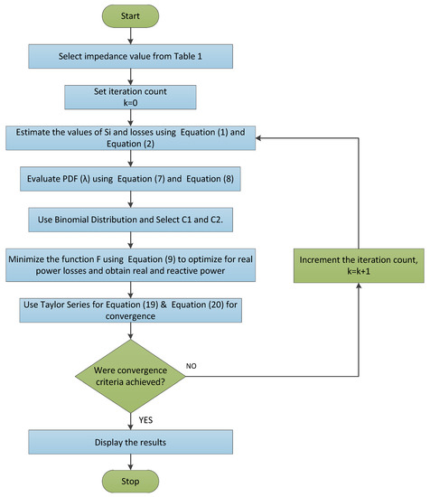
Figure 1.
Flowchart of heuristic PDF method.
The load representations for CPLF and CILF are given by Equations (21)–(23):
where
Vo is rated voltage of a particular bus while x and y are constant load parameter and its values are shown in Table 1.

Table 1.
Constant parameter value for CPLF and CILF.
The constant values of x and y are taken for power load and impedance load; that is why they are called constant power load and constant impedance load.
The sensitivity and accuracy can be represented as in pu and in pu, respectively.
2.2. Performance Evaluation for Standard IEEE Tested 33 Bus Systems Using Heuristic PDF
The effectiveness of the proposed scheme using the conventional method is being tested initially on the standard IEEE 33 bus test system for CPLF and CILF [36,37]. The typical diagram of the IEEE 33 bus test system is shown in Figure 2 [37].
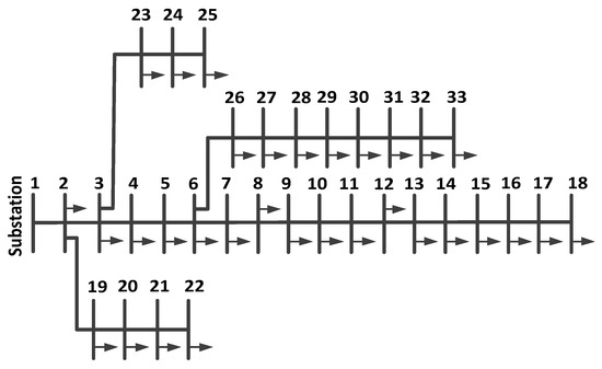
Figure 2.
IEEE 33 bus test system.
The IEEE 33 bus test system is modelled in MATLAB with location of fault from 0–90 km. This system consists of 33 buses and 32 lines and has 12.66 kV, 3.715 MW, and 2.3 MVar load size. Thirty percent of the entire load is the size of the source unit used. The source unit voltage is 12.66 kV and the system’s lower and upper voltage is set between 0.95 pu and 1.05 pu with standard internal parameters as given in [37]. Bus 1 is considered as the slack bus or main substation. The internal parameters of the IEEE 33 bus test system are shown in [36].
The proposed design illustrated from Equations (1)–(23) is applied on the standard IEEE 33 bus test system for estimation of location of DG using the heuristic PDF method. By using these equations, the parameters such as real power loss, accuracy, and sensitivity are estimated as shown in Table 2. The design part has already been discussed in the previous section.
Table 2.
Performance parameter of DG at different locations for the IEEE 33 bus system with the heuristic PDF method for CPLF and CILF.
2.3. Genetic Algorithm
GA is used to find the best location of DG in the IEEE 33 bus system. It involves reproduction, crossover, and mutation. Its procedure can be illustrated by the flowchart as shown in Figure 3. The process begins with selection of a binary string as shown by Equation (24), the parameters for which are assumed as follows:
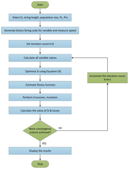
Figure 3.
Flowchart representing the GA.
Population size: 6, length of the complete string: 8, crossover probability, Pc = 0.9, mutation probability, Pm = 0.02.
where r is the iteration count. The application of iteration in Equation (24) results in Equations (25) and (26):
α is step size which is equal to 0.5.
Figure 4 and Figure 5 show real power loss at bus 17 for CPLF and CILF using GA. The performance parameter for finding the DG location can be analyzed from Table 2 and Table 3 at different DG locations in the IEEE 33 bus system using heuristic PDF and GA methods for both CPLF and CILF. Figure 6 and Figure 7 provide the performance parameter comparison of GA with the heuristic method at different buses for CPLF and CILF. Moreover, in order to have comprehensive analysis and comparison for the DG location with GA and heuristic pdf, the results are compared with those obtained with the ant-lion optimization algorithm [42], coyote optimizer [43], modified sine-cosine algorithm [44], and particle swarm optimization [45]. The performance parameter evaluation for the estimation of DG location by using the ant-lion optimization algorithm [42], coyote optimizer [43], modified sine-cosine algorithm [44], and particle swarm optimization [45] is shown in Table 4, Table 5, Table 6 and Table 7 for CPLF and CILF type of load.
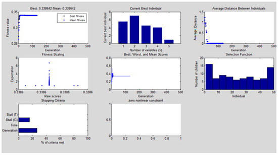
Figure 4.
Real power loss at bus 17 after 150 iterations using GA for CPLF.

Figure 5.
Real power loss at bus 17 after 155 iterations using GA for CILF.
Table 3.
Performance parameter of DG at different locations for the modified IEEE 33 bus system with GA for CPLF and CILF.
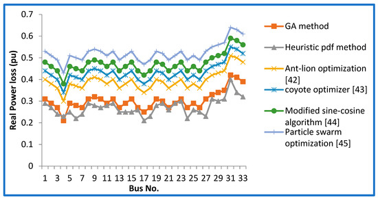
Figure 6.
Real power loss comparison for CPLF.
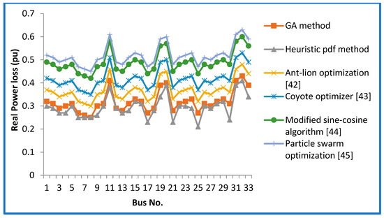
Figure 7.
Real power loss comparison for CILF.
Table 4.
Performance parameter of DG at different locations for the IEEE 33 bus system with the ant-lion optimization algorithm [42] for CPLF and CILF.
Table 5.
Performance parameter of DG at different locations for the IEEE 33 bus system with the coyote optimizer [43] for CPLF and CILF.
Table 6.
Performance parameter of DG at different locations for the IEEE 33 bus system with the modified sine-cosine algorithm [44] for CPLF and CILF.
Table 7.
Performance parameter of DG at different locations for the IEEE 33 bus system with the particle swarm optimization [45] for CPLF and CILF.
From Table 2, Table 3, Table 4, Table 5, Table 6 and Table 7, it is observed that the selection of DGs location is better found under GA for CPLF and CILF in comparison to other methods. By comparing the real power loss, sensitivity, and accuracy, it can be concluded that bus 17 is the best location for the placement of DG for both CPLF and CILF. In the sequence manner, bus 3 and bus 4 are the second and third position of placing the next two DGs. The comparative results for positioning of three DGs with different methods are shown in Table 8.
Table 8.
Performance comparison among different methods.
2.4. Optimal Sizing of DG
After deciding the optimal location of three DGs, it is also required to check the DG size to confirm its placement at bus 17. DG size is estimated from Table 9, Table 10 and Table 11 by using heuristic pdf, GA, ant-lion optimization algorithm [42], coyote optimizer [43], modified sine-cosine algorithm [44], and particle swarm optimization [45] for both CPLF and CILF type of load. It is observed that the size of DG when placed at bus 17 is found to be the minimum. The relative comparison of DG size for bus 17, 4, and 3 is shown in Table 12. The minimal size of DG is obtained under GA as compared to the heuristic method. Figure 8, Figure 9 and Figure 10 illustrate the real power and Figure 11 illustrates the reactive power at bus 17 for both CPLF and CILF. From the results, it is confirmed that bus 17 is the best choice for the location and optimum sizing of DG is also obtained here. Subsequently, bus 3 and bus 4 have the appropriate size of DGs, which assures the confirmation of the DG location. The location and size of three DGs at the allotted location in the IEEE 33 bus system are shown in Figure 12.
Table 9.
DG size comparison for CPLF and CILF using GA and heuristic PDF.
Table 10.
DG size comparison for CPLF and CILF using the ant-lion optimization algorithm [42] and coyote optimizer [43].
Table 11.
DG size comparison for CPLF and CILF using the modified sine-cosine algorithm [44] and particle swarm optimization [45].
Table 12.
DG size comparison at the three best bus locations.
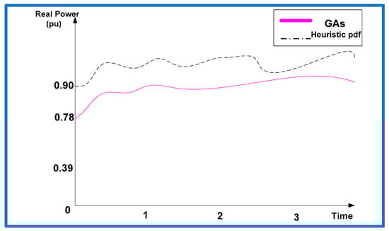
Figure 8.
Real power at bus 17 after150 iterations for CPLF.
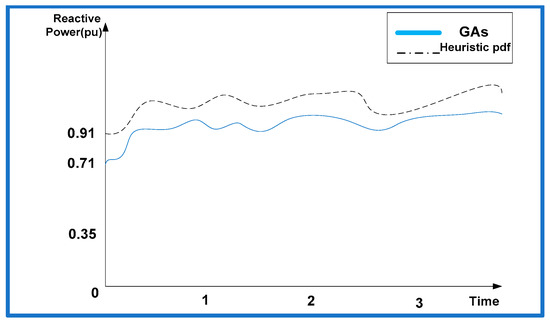
Figure 9.
Reactive power at bus 17 after 150 iterations using GA for CPLF.
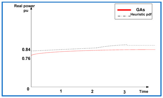
Figure 10.
Real power at bus 17 after 155 iterations using GA for CILF.
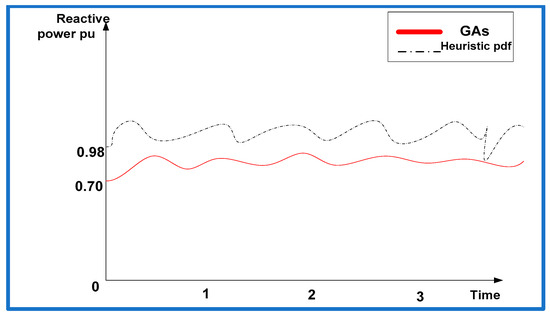
Figure 11.
Reactive power at bus 17 after 155 iterations using GA for CILF.
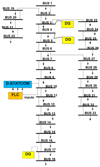
Figure 12.
Layout of the IEEE 33 bus system with allocated positioning and sizing of DG and D-STATCOM.
3. Positioning and Impact of D-STATCOM
The positioning and impact of D-STATCOM in the IEEE-33 bus system have to be assessed for improving the power quality performance parameters such as THD and voltage profile. The rating of D-STATCOM is 1 pu reactive power. In order to improve power quality performance, control of D-STATCOM is decided by using the fuzzy logic controller. In this article, only one D-STATCOM is used, so it has to be connected at that bus where large distortions are present. In order to define the inputs and output of FLC, Equation (9) is further used. Now, we differentiate Equation (9) to obtain the optimal solution.
Equation (27) enables us to differentiate J with respect to E as given in Equation (28). After differentiating, Equation (29) is obtained:
By arranging the terms in Equation (29) and by taking log on both sides, the value of E is obtained as given by Equation (30).
Equation (30) gives the optimal solution. Now, the inputs to FLC are error (E) and change in error (ΔE) which are shown in Equation (31) as:
The detailed structure of the D-STATCOM-based FLC controller is shown in Figure 13 and Figure 14. In Figure 13, distorted real and reactive power is measured and passes through the PID controller which generates the measured complex power. The measured complex power is compared with its reference value which produces error. The error and derivative of error act as inputs to FLC. The actual design of FLC for D-STATCOM switching is shown in Figure 14. The output of FLC is reference voltage which is compared with reference value and generates pulses for switching the D-STATCOM. In the same pattern, ΔE can be expressed in standard form.
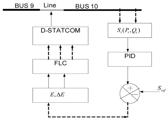
Figure 13.
Structure of D-STATCOM-based FLC controller.

Figure 14.
Switching of D-STATCOM.
In order to design rules of the fuzzy set, a 7 × 7 matrix is taken so that the model will have more precise and better results. This means both inputs have seven membership functions. Using Cramer’s product rule, FLC rule is designed as shown in Figure 15 and its surface view is shown in Figure 16. Table 13 and Table 14 show the notification of membership function for first input, as initial error E is around 0.12 and mapping of input with output, respectively.
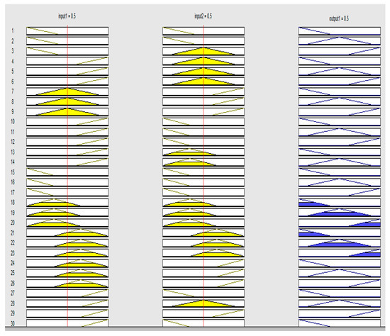
Figure 15.
Fuzzy rules of FLC.
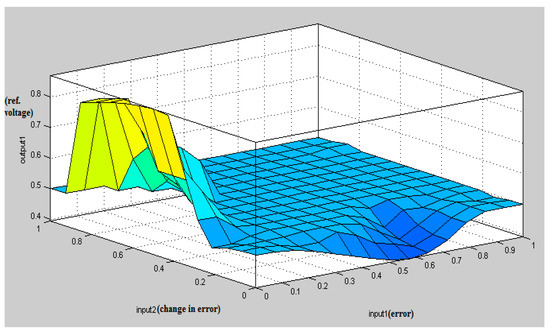
Figure 16.
Surface view of FLC between inputs and output.
Table 13.
Mathematical notation of input and output.
Table 14.
Mapping of output with input.
From Table 13 and Table 14, it can be demonstrated that, under certain parameters, a precise control of objectives can be achieved using fuzzy observations, mapping, and control, if the observations become sufficiently accurate as the goal is approached.
The seven membership functions corresponding to the first input are shown in Equation (32) and these seven membership functions are taken from x1 to x7. The seven membership functions are chosen in order to have better and more precise results. The nature of the membership function is triangular and input is split into seven membership functions. Each membership function from x1 to x7 is assigned with values in the numerator as shown in Equation (32).
Dividing Equation (32) by 0.12, Equation (33) is obtained as:
Notification of membership function for the second input is given in Equation (34):
From the Cartesian product rule:
Further membership function is taken as:
Table 15 gives the comparative analysis of voltage profile at different buses with different existing techniques and D-STATCOM-based FLC for both CPLF and CILF load; whereas computational expression of THD is given by Equation (35).
Table 15.
Voltage (pu) comparisons at different buses with D-STATCOM-based FLC and existing methods.
Table 16 gives the comparative analysis of THD (%) of real power different buses with different existing techniques and D-STATCOM-based FLC for both CPLF and CILF load.
where ‘g’ is distortion factor which is defined as ratio of rms fundamental harmonic value to rms value of voltage.
Table 16.
THD (%) of real power comparison at different buses with D-STATCOM-based FLC and existing methods.
Now, a suitable location for D-STATCOM at a particular bus has to be decided. From Figure 9 and Figure 10, it can be inferred that voltage profile and THD (%) of the real power at bus 10 are found to be worst with existing methods such as harmony search algorithm [4], ant colony algorithm [9], and big-bang–crunch method [30] for both CPLF and CILF. Therefore, D-STATCOM is placed at bus 10. Figure 17 and Figure 18 show the voltage (pu) comparisons at bus 10 for CPLF and CILF. It is also observed that switching of D-STATCOM with FLC improves its voltage profile and THD (%). This means that switching of D-STATCOM with FLC helps to improve the performance parameters in comparison to existing methods. The comparison of voltage profile and THD (%) of real power at bus 10 with existing techniques and D-STATCOM-based FLC is shown in Table 17 and Table 18 and its graphical comparison is shown in Figure 19 and Figure 20.
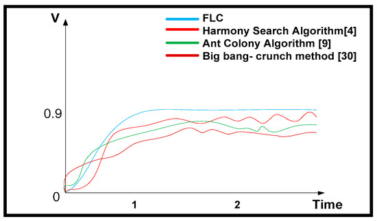
Figure 17.
Voltage comparison at bus 10 for CPLF.
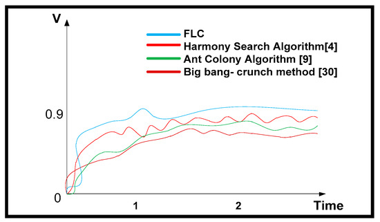
Figure 18.
Voltage comparison at bus 10 for CILF.
Table 17.
Comparative analysis for voltage (pu) at bus 10 for both types of load.
Table 18.
Comparative analysis for THD (%) of real power at bus 10 for both types of load.
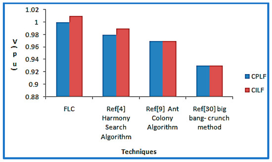
Figure 19.
Graphical voltage comparison at bus 10 with different methods for CPLF and CILF.
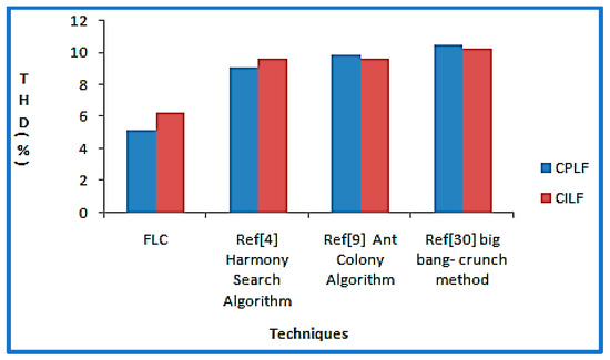
Figure 20.
Graphical THD (%) of real power comparison at bus 10 with different methods for CPLF and CILF.
4. Result Summary
This article shows location and sizing of three DGs for CPLF and CILF types of load using GA and heuristic PDF method. The location of the DGs was obtained based on three different parameters such as line power losses, accuracy, and sensitivity. The application of GA method shows that all three parameters of DG placement are improved in comparison with the heuristic PDF method as well as existing methods such as ant-lion optimization algorithm, coyote optimizer, modified sine-cosine algorithm, and particle swarm optimization. It is also observed that after obtaining optimal location for DG placement at bus 17, optimal sizing for DG has been determined among all buses and the most optimal solution turns out to be at bus 17 in terms of minimum real and reactive power. It is found that determination of size of DG is quite satisfactorily observed under GA in comparison to the heuristic PDF method, ant-lion optimization algorithm, coyote optimizer, modified sine-cosine algorithm, and particle swarm optimization. Subsequently, bus 3 and bus 4 are the second and third best locations for placement of DGs with optimal size. Now, positioning of D-STATCOM on the IEEE 33 bus system is assessed in such a way that the bus with the worst performance in terms of THD and voltage profile has to be detected. On the basis of the analysis performed, bus 10 is found to be most suitable for locating the D-STATCOM. Afterwards, in order to improve the THD and voltage profile, switching of D-STATCOM is performed through FLC, consequently showing superiority over other existing methods. The current research will provide considerable expertise and also acts as a guide for researchers, including utility engineers, regarding problems to be addressed in order to optimize the size and position of DG units within electrical power systems. The metaheuristic computation approaches recently unveiled could be implemented for optimal design and fitting of DG in network delivery in future.
5. Conclusions
This article presents the optimal location and sizing of three DGs in the IEEE 33 bus test system by using the heuristic PDF method and GA for CPLF and CILF. Associated bus locations are examined for analysis of the impact of optimal placement and size of DG. The optimal locations of DGs are selected in terms of performance parameters such as line power losses, sensitivity, and accuracy while sizing of DG is obtained in terms of real and reactive power. It is evident that the parameters such as voltage profile, line power loss, accuracy, sensitivity, THD, etc. are improved with the GA method as compared to the heuristic PDF method and other existing methods such as the ant-lion optimization algorithm, coyote optimizer, modified sine-cosine algorithm, and particle swarm optimization. It is also confirmed that determining DG size is resolved quite satisfactorily with the GA method in terms of real power and reactive power, rather than heuristic PDF and other existing methods. Further positioning of D-STATCOM is being decided on the basis of bus having the worst voltage profile and THD (%) of real power. The D-STATCOM is controlled with FLC which gives improved voltage and less THD of real power in comparison to existing techniques.
Author Contributions
Conceptualization, P. and M.S.; formal analysis, P., A.A. and S.S.M.G.; funding acquisition, S.S.M.G.; investigation, A.A.; methodology, P., M.S. and A.A.; project administration, P., A.A. and S.S.M.G.; resources, S.S.M.G.; software, P. and M.S.; supervision, P., A.S.S. and M.S.; validation, P. and M.S.; visualization, P., A.S.S., M.S. and A.A.; writing—original draft, P., A.S.S. and M.S.; writing—review and editing, P., A.A. and S.S.M.G. All authors have read and agreed to the published version of the manuscript.
Funding
This research was funded by TAIF UNIVERSITY RESEARCHERS SUPPORTING PROJECT, grant number TURSP-2020/34”, Taif University, Taif, Saudi Arabia, and “The APC was funded by SHERIF GHONEIM”.
Data Availability Statement
All data generated or analysed during this study are included in this research article and any relevant information related to the current study are available from the corresponding author on reasonable request.
Acknowledgments
The authors would like to acknowledge the financial support received from Taif University Researchers Supporting Project Number (TURSP-2020/34), Taif University, Taif, Saudi Arabia.
Conflicts of Interest
The authors declare no conflict of interest.
Abbreviations
| DG | Distributed generator | δi | Load angle |
| CPLF | Constant power load flow | θi | Impedance angle at ‘i’ bus |
| CILF | Constant impedance load flow | θj | Impedance angle at ‘j’ bus |
| FLC | Fuzzy logic controller | Ɛ | Tolerance limit |
| GA | Genetic Algorithm | yr | Initial code of string |
| D-STATCOM | Distribution static compensator | λ | Difference between measured and reference power |
| THD | Total harmonic distortion | σ | Standard deviation |
| Probability distribution method | E | Error | |
| PWM | Pulse width modulation | NB | Negative big |
| Sij | Complex power between 2 buses i & j | NM | Negative medium |
| Pij | Real power between 2 buses i & j | NS | Negative small |
| Qij | Reactive power between 2 buses i & j | PB | Positive big |
| Sloss | Complex power loss | PM | Positive medium |
| Gij | Conductance between i & j bus | PS | Positive small |
| Bij | Susceptance between ‘i’ & ‘j’ bus | ZS | Zero |
References
- Bernardon, D.P.; Mello, A.P.C.; Pfitscher, L.L.; Canha, L.N.; Abaide, A.R.; Ferreira, A.A. Real-time reconfiguration of distribution network with distributed generation. Electr. Power Syst. Res. 2014, 107, 59–67. [Google Scholar] [CrossRef]
- Chicco, G.; Mazza, A. An overview of the probability-based methods for optimal electrical distribution system reconfiguration. In Proceedings of the Fourth International Symposium on Electrical and Electronics Engineering (ISEEE), Galați, Romania, 11–13 October 2013; pp. 1–10. [Google Scholar]
- Chan, C.-M.; Liou, H.-R.; Lu, C.-N. Operation of distribution feeders with electric vehicle charging loads. In Proceedings of the 2012 IEEE 15th International Conference on Harmonics and Quality of Power (ICHQP), Hong Kong, China, 17–20 June 2012; pp. 695–700. [Google Scholar]
- Ganguly, S.; Samajpati, D. Distributed generation allocation on radial distribution networks under uncertainties of load and generation using genetic algorithm. IEEE Trans. Sustain. Energy 2015, 6, 688–697. [Google Scholar] [CrossRef]
- Martins, V.F.; Borges, C.L.T. Active distribution network integrated planning incorporating distributed generation and load response uncertainties. IEEE Trans. Power Syst. 2011, 26, 2164–2172. [Google Scholar] [CrossRef]
- Salman, N. Practical mitigation of voltage sag in distribution networks by combining network reconfiguration and DSTATCOM. In Proceedings of the IEEE International Conference on Power and Energy (PECON2010), Kualalumpur, Malaysia, 29 November–1 December 2010. [Google Scholar]
- Li, G.; Shi, D.; Duan, X.; Li, H.; Yao, M. Multiobjective optimal network reconfiguration considering the charging load of PHEV. In Proceedings of the Power and Energy Society General Meeting, San Diego, CA, USA, 22–26 July 2012; IEEE: New York, NY, USA, 2012; pp. 1–8. [Google Scholar]
- Pandi, V.R.; Zeineldin, H.H.; Xiao, W. Determining optimal location and size of distributed generation resources considering harmonic and protection coordination limits. IEEE Trans. Power Syst. 2013, 28, 1245–1254. [Google Scholar] [CrossRef]
- Swarnkar, A.; Gupta, N.; Niazi, K.R. Optimal placement of fixed and switched shunt capacitors for large-scale distribution systems using genetic algorithms. In Proceedings of the Innovative Smart Grid Technologies Conf. Europe (ISGT Europe), Gothenburg, Sweden, 11–13 October 2010; IEEE: New York, NY, USA, 2010; pp. 1–8. [Google Scholar]
- Farahani, V.; Vahidi, B.; Abyaneh, H.A. Reconfiguration and capacitor placement simultaneously for energy loss reduction based on an improved reconfiguration method. IEEE Trans. Power Syst. 2012, 27, 587–595. [Google Scholar] [CrossRef]
- Tuladhar, S.R.; Singh, J.G.; Ongsakul, W. Multi-objective approach for distribution network reconfiguration with optimal DG power factor using NSPSO. IET Gener. Transm. Distrib. 2016, 10, 2842–2851. [Google Scholar] [CrossRef]
- Jasthi, K.; Das, D. Simultaneous distribution system reconfiguration and DG sizing algorithm without load flow solution. IET Gener. Transm. Distrib. 2017, 12, 1303–1313. [Google Scholar] [CrossRef]
- Kalambe, S.; Agnihotri, G. Loss minimization techniques used in distribution network: Bibliographical survey. Renew. Sust. Energy Rev. 2014, 29, 184–200. [Google Scholar] [CrossRef]
- Muhammad, M.A.; Mokhlis, H.; Naidu, K.; Franco, J.F.; Illias, H.A.; Wang, L. Integrated data base approach in multi-objective network reconfiguration for distribution system using discrete optimisation techniques. IET Gener. Transm. Distrib. 2018, 12, 976–986. [Google Scholar] [CrossRef] [Green Version]
- Lalitha, M.P.; Reddy, V.V.; Usha, V. Optimal Dg placement for minimum real power loss in radial distribution system using PSO. J. Theor. Appl. Inf. Technol. 2010, 13, 107–116. [Google Scholar]
- Gözel, T.; Hocaoglu, M.H. An analytical method for the sizing and siting of distributed generators in radial systems. Electr. Power Syst. Res. 2009, 79, 912–918. [Google Scholar] [CrossRef]
- Zhang, S.; Cheng, H.; Li, K.; Bazargan, M.; Yao, L. Optimal siting and sizing of intermittent distributed generators in distribution system. IEEJ Trans. Electr. Electron. Eng. 2015, 10, 628–635. [Google Scholar] [CrossRef]
- Kumar, K.S.; Jayabarathi, T. Power system reconfiguration and loss minimization for a distribution systems using bacterial foraging optimization algorithm. Int. J. Electr. Power Energy Syst. 2012, 36, 13–17. [Google Scholar] [CrossRef]
- Kaur, M.; Ghosh, S. Network reconfiguration of unbalanced distribution networks using fuzzy-firefly algorithm. Appl. Soft Comput. 2016, 49, 868–886. [Google Scholar] [CrossRef]
- Hung, D.Q.; Mithulananthan, N. Multiple distributed generator placement in primary distribution networks for loss reduction. IEEE Trans. Ind. Electron. 2013, 60, 1700–1708. [Google Scholar] [CrossRef]
- Angelim, J.H.; Affonso, C.M. Impact of distributed generation technologyand location on power system voltage stability. IEEE Latin Am. Trans. 2016, 14, 1758–1765. [Google Scholar] [CrossRef]
- Wu, Y.-K.; Lee, C.-Y.; Liu, L.-C.; Tsai, S.H. Study of reconfiguration for the distribution system with distributed generators. IEEE Trans. Power Deliv. 2010, 25, 1678–1685. [Google Scholar] [CrossRef]
- Liu, K.-Y.; Sheng, W.; Liu, Y.; Meng, X. A network reconfiguration method considering data uncertainties in smart distribution networks. Energies 2017, 10, 618. [Google Scholar] [CrossRef] [Green Version]
- Rao, R.; Ravindra, K.; Satish, K.; Narasimham, S.V.L. Power loss minimization in distribution system using network reconfiguration in the presence of distributed generation. IEEE Trans. Power Syst. 2013, 28, 317–325. [Google Scholar] [CrossRef]
- Prabha, D.R.; Jayabarathi, T.; Umamageswari, R.; Saranya, S. Optimal location and sizing of distributed generation unit using intelligent water drop algorithm. Sustain. Energy Technol. Assess. 2015, 11, 106–113. [Google Scholar] [CrossRef]
- Rezk, H.; Abdelkareem, M.A.; Ghenai, C. Performance evaluation and optimal design of stand-alone solar PV-battery system for irrigation in isolated regions: A case study in Al Minya (Egypt). Sustain. Energy Technol. Assess. 2019, 36, 100556. [Google Scholar] [CrossRef]
- El-Zonkoly, A.M. Optimal placement of multi-distributed generation units including different load models using particle swarm optimization. Swarm Evol. Comput. 2011, 1, 50–59. [Google Scholar] [CrossRef]
- Naik, S.G.; Khatod, D.K.; Sharma, M.P. Optimal allocation of combined DG and capacitor for real power loss minimization in distribution networks. Int. J. Electr. Power Energy Syst. 2013, 53, 967–973. [Google Scholar] [CrossRef]
- Sandeep, K.; Ganesh, K.; Jaydev, S. A MINLP technique for optimal placement of multiple DG units in distribution systems. Electr. Power Energy Syst. 2014, 63, 609–617. [Google Scholar]
- Othman, M.M.; Walid, E.; Yasser, G.H.; Almoataz, Y.A. Optimal placement and sizing of distributed generators in unbalanced distribution systems using supervised big bang-big crunch method. IEEE Trans. Power Syst. 2015, 30, 911–919. [Google Scholar] [CrossRef]
- Naresh, A.; Mahat, P.; Mithulananthan, N. An analytical approach for DG allocation in primary distribution network. Int. J. Electr. Power Energy Syst. 2006, 28, 669–678. [Google Scholar]
- Mithulananthan, N.; Oo, T.; Phu, L.V. Distributed generator placement in power distribution system using genetic algorithm to reduce losses. TIJSAT 2004, 9, 55–62. [Google Scholar]
- Hamed, S.H. Intelligent water drops algorithm: A new optimization method for solving the multiple knapsack problem. Int. J. Intell. Comput. Cybern. 2008, 1, 193–212. [Google Scholar]
- Muqbel, A.; Elsayed, A.H.; Abido, M.A.; Mantawy, A.A.; Al-Awami, A.T.; El-Hawary, M. Optimal Sizing and Location of Solar Capacity in an Electrical Network Using Lightning Search Algorithm. Electr. Power Compon. Syst. 2020, 47, 1247–1260. [Google Scholar] [CrossRef]
- Siahbalaee, J.; Rezanejad, N.; Gharehpetian, G.B. Reconfiguration and DG Sizing and Placement Using Improved Shuffled Frog Leaping Algorithm. Electr. Power Compon. Syst. 2020, 47, 1475–1488. [Google Scholar] [CrossRef]
- Baran, M.E.; Wu, F.F. Network reconfiguration in distribution systems for loss reduction and load balancing. IEEE Trans. Power Deliv. 1989, 4, 1401–1407. [Google Scholar] [CrossRef]
- Bagherinezhad, A.; Palomino, A.D.; Li, B.; Parvania, M. Spatio-Temporal Electric Bus Charging Optimization with Transit Network Constraints. IEEE Trans. Ind. Appl. 2020, 56, 5741–5749. [Google Scholar] [CrossRef]
- Elmetwaly, A.H.; Eldesouky, A.A.; Sallam, A.A. An Adaptive D-FACTS for Power Quality Enhancement in an Isolated Microgrid. IEEE Access 2020, 8, 57923–57942. [Google Scholar] [CrossRef]
- Castiblanco-Pérez, C.M.; Toro-Rodríguez, D.E.; Montoya, O.D.; Giral-Ramírez, D.D. Optimal Placement and Sizing of D-STATCOM in Radial and Meshed Distribution Networks Using a Discrete-Continuous Version of the Genetic Algorithm. Electronics 2021, 10, 1452. [Google Scholar] [CrossRef]
- Yuvaraj, T.; Devabalaji, K.; Ravi, K. Optimal Placement and Sizing of DSTATCOM Using Harmony Search Algorithm. Energy Procedia 2015, 79, 759–765. [Google Scholar] [CrossRef] [Green Version]
- Rukmani, D.K.; Thangaraj, Y.; Subramaniam, U.; Ramachandran, S.; Madurai Elavarasan, R.; Das, N.; Baringo, L.; Imran Abdul Rasheed, M. A New Approach to Optimal Location and Sizing of DSTATCOM in Radial Distribution Networks Using Bio-Inspired Cuckoo Search Algorithm. Energies 2020, 13, 4615. [Google Scholar] [CrossRef]
- Moayedi, H.; Mosavi, A. Synthesizing Multi-Layer Perceptron Network with Ant lion Biogeography-Based Dragonfly Algorithm Evolutionary Strategy Invasive Weed and League Champion Optimization Hybrid Algorithms in Predicting Heating Load in Residential Buildings. Sustainability 2021, 13, 3198. [Google Scholar] [CrossRef]
- Kamel, S.; Amin, A.; Selim, A. Application of coyote optimizer for Optimal DG Placement in Radial Distribution Systems. In Proceedings of the 2019 International Conference on Computer, Control, Electrical, and Electronics Engineering ICCCEEE, Khartoum, Sudan, 21–23 September 2019. [Google Scholar]
- Qu, C.; Zeng, Z.; Dai, J.; Yi, Z.; He, W. A Modified Sine-Cosine Algorithm Based on Neighborhood Search and Greedy Levy Mutation. Comput. Intell. Neurosci. 2018, 2018, 4231647. [Google Scholar] [CrossRef]
- Al-Masri, H.M.K.; Al-Sharqi, A.A.; Magableh, S.K.; Al-Shetwi, A.Q.; Abdolrasol, M.G.M.; Ustun, T.S. Optimal Allocation of a Hybrid Photovoltaic Biogas Energy System Using Multi-Objective Feasibility Enhanced Particle Swarm Algorithm. Sustainability 2022, 14, 685. [Google Scholar] [CrossRef]
Publisher’s Note: MDPI stays neutral with regard to jurisdictional claims in published maps and institutional affiliations. |
© 2022 by the authors. Licensee MDPI, Basel, Switzerland. This article is an open access article distributed under the terms and conditions of the Creative Commons Attribution (CC BY) license (https://creativecommons.org/licenses/by/4.0/).