
Analysis on the Mechanism and Influencing Factors of the Coordinated Development of Economy and Environment in China’s Resource-Based Cities


Abstract
:1. Introduction
2. Literature Review
3. Mechanism Analysis and Hypothesis
- When λC(t) > ΦC(t)/β(t), ΦC(t) < λC(t)/α(t), the economy can continue to develop, but the ecological environment will have reached the maximum carrying capacity and cannot continue for growth; the economic development of resource-based cities will ultimately prevail.
- When λC(t) < ΦC(t)/β(t), ΦC(t) > λC(t)/α(t), the result of the competition is that the ecological environment wins, and the urban economic development stagnates or even regresses.
- When λC(t) < ΦC(t)/β(t), ΦC(t) < λC(t)/α(t), the two enter a stable state of coexistence and development, and E is the equilibrium point (Ind(t), Eco(t)).
- When λC(t) > ΦC(t)/β(t), ΦC(t) > λC(t)/α(t), the two are in an unstable state of competition, and both sides have the possibility of winning.
4. Research Methods
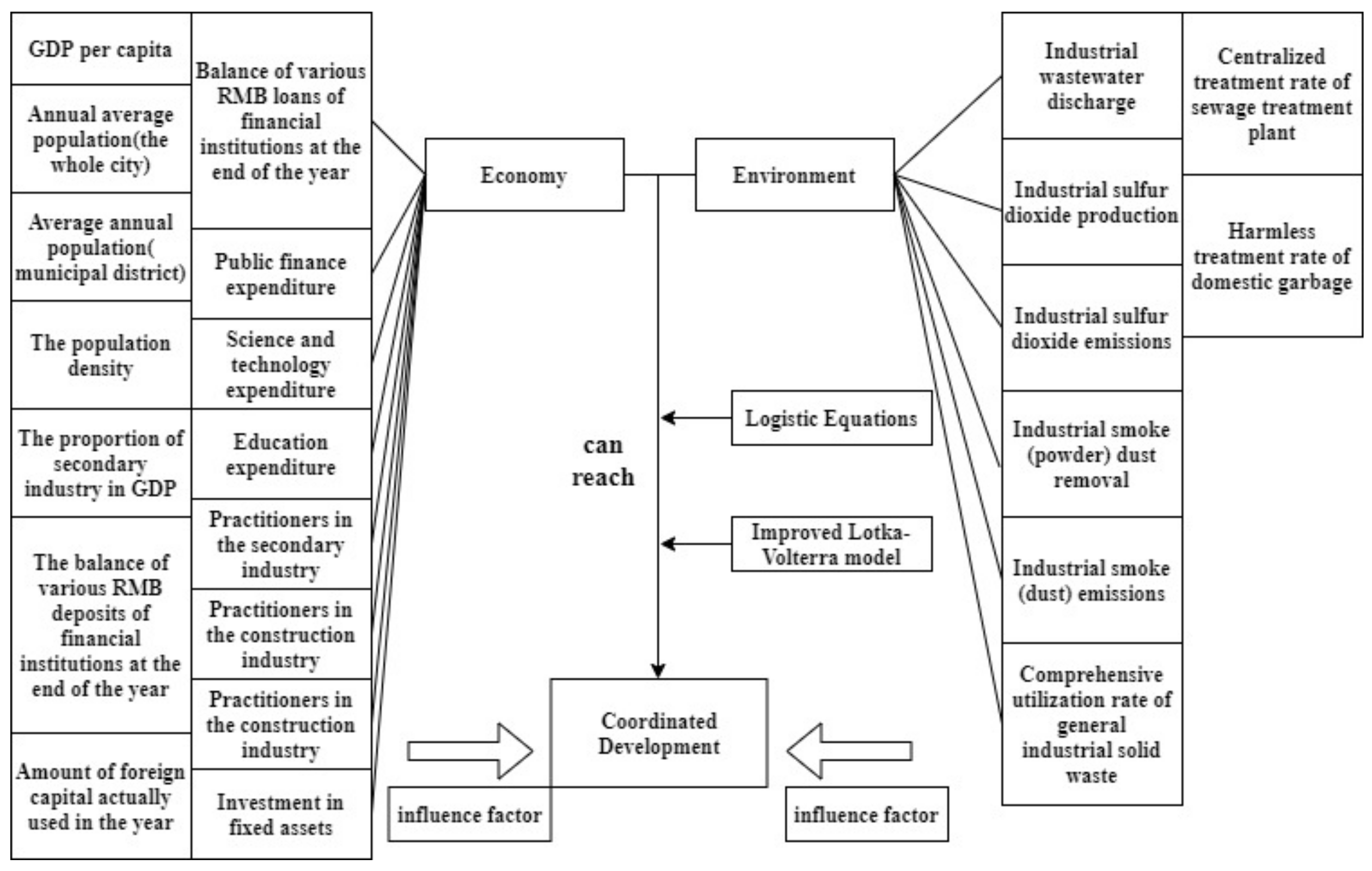
4.1. Constructing an Evaluation Index System
4.1.1. Evaluation Index System of Environmental Carrying Capacity of Resource-Based Cities
4.1.2. Resource-Based City Economic Strength Evaluation Index System
- (1)
- City GDP.The city’s GDP is a basic indicator for evaluating the current status of the city’s economic development, reflecting the total annual economic development of a city. This article uses per capita GDP to evaluate the economy.
- (2)
- Economic growth rate.Economic growth rate reflects the dynamic index of resource-based city economic development while per capita GDP reflects the stock index of resource-based city economic development.
- (3)
- Proportion of added value by industry.The proportion of sub-industry added value reflects the degree of importance of each industry in the urban economy and is a common indicator that reflects the status of the industrial structure in urban economic development. According to Clark’s theorem, the advancement and rationalization of industrial development is a process of transition from industrialization to post-industrialization. Therefore, the main indicators to measure the industrial structure of resource-based cities are the proportion of the added value of the secondary industry and the proportion of the added value of the tertiary industry.
- (4)
- Disposable income of residents.The disposable income of residents reflects the income of residents, which is another indicator that reflects the economic development of resource-based cities. This article uses standardized per capita disposable income as the evaluation index.
- (1)
- Investment in fixed assets.The situation of urban GDP and industrial added value reflects the economic output capacity of resource-based cities, while fixed resource investment reflects the continuity of economic development.
- (2)
- Unemployment rate.As a negative evaluation indicator of economic development, the unemployment rate reflects the stability and dynamics of economic development more clearly, compared to indicators such as the number of employees.
- (3)
- Urban public service level.Urban public financial expenditure reflects the level of social and public service in the city. The higher the level of public financial expenditure is, the higher the level of urban construction and public services is, the more stably the city develops, the stronger the driving force of the city’s development grows.
- (4)
- The driving force of science and technology development.From the perspective of urban input factors, according to the Cobb–Douglas production function, the traditional input factors are mainly labor and capital, but the rate of technological progress and technological factors have a stronger effect on urban economic development. The science and technology expenditure index reflects the city’s investment in science and technology. The higher the value, the more it reflects the importance of local technological progress, which further indicates the city’s technological development potential and the city’s long-term development momentum.
4.2. Evaluation Method
- (1)
- Construction of the index data matrix:where, is the value of the j-th index of the i-th scheme. If the indicator is negative, the data should be transformed to be non-negative.
- (2)
- Data standardization:Positive indicators:Negative indicators:Perform data translation to avoid meaningless logarithm when calculating entropy:
- (3)
- Calculate the proportion of the i-th scheme under the j-th index in this index:
- (4)
- Calculate the entropy of the j-th index:
- (5)
- Calculate the difference coefficient:
- (6)
- Calculate weight:
- (7)
- Calculate the comprehensive score of each scheme:
4.3. Empirical Verification Method
- (1)
- With the indicators related to economic development and urban, comprehensive carrying capacity set as independent variables, the resource-based city economy and environment coupling coordination degree as the dependent variable, a basic regression model was established to explore the effect of these variables on resource-based city economy and environment coupling coordination degree effect.
- (2)
- Resource-based cities mainly include four types: mature, growth, decline, and regeneration(according to the standards issued by the State Council). This paper again uses the basic regression model to carry out regression analysis on the data of mature resource-based cities to further verify the robustness of the regression model. (Because the data of growth-declining and renewable resource-based cities is not sufficient to do effective regression, this article only uses the data of mature resource-based cities).
4.3.1. Calculation Model of Coupling and Coordination Degree of Resource-Based City Economy and Environment
4.3.2. Basic Regression Model
5. Data Source and Variable Description
5.1. Data Source
5.2. Variable Description
6. Analysis of Empirical Results
6.1. Analysis of Environmental Carrying Capacity of Resource-Based Cities
6.2. Analysis of the Economic Strength of Resource-Based Cities
6.3. Analysis of Coupling Coordination Degree between Economy and Environment in Resource-Based Cities

6.4. Analysis of Factors Affecting the Coordinated Development of Environment and Economy in Resource-Based Cities
6.5. Analysis of the Economic Strength of Resource-Based Cities
7. Discussion
- (1)
- The 109 prefecture-level resource-based cities, recognized by the sustainable development plan of resource-based cities of the State Council, are of various resource conditions, including coal, metal mines, oil, etc. With different resource endowments, these cities show different environmental pollution emission intensities. Thus, these cities are facing different environmental pollution emission pressures. In order to solve this problem, different resource-based cities have issued different measures. In this study, only the common characteristics of resource-based cities were considered, with the individual characteristics which cannot reflect the impact of different resource endowment conditions ignored.
- (2)
- The resource-based cities in China are mostly the prefecture-level cities of various provinces and regions, which are often not the core cities in their provinces or regions. Many of them are of less advanced urban development and short development cycle, resulting in great uncertainty in the environmental- and industrial-related data collected. Therefore, the research indicators and data selected in this study also have certain limitations. As the environmental pollution emission data of specific industrial sectors cannot be obtained, the strength, proportion, and employment of each branch industrial sector of resource-based cities cannot be analyzed.
- (1)
- In the following research, new classification methods can be adopted. For example, the resource endowment characteristic indicators and data can be collected according to the different resource conditions of the research object. Thus, an in-depth comparison and analysis of the coordinated development characteristics of economic systems and ecological environment systems in different resource-based cities can be conducted, combined with the commonness analysis of this paper.
- (2)
- The scope of index data collection can be expanded. Through abstract field investigation, the microdata of the resource-based urban economic system and ecological environment system can be collected so as to modify the research data of this paper and more accurately reflect the actual situation of the resource-based urban economic system and ecological environment system, thus enhancing the microdata basis of this paper.
8. Conclusions
- (1)
- The environmental carrying capacity of resource-based cities is at a medium level, among which water and land resources are relatively poor. Most resource-based cities have only just reached the medium carrying capacity level. Resource-based cities of different development types do not show obvious differences in environmental carrying capacity and are basically at the same carrying capacity level. However, by a numerical comparison, a shift in it occurs from growth-oriented resource-based cities to mature, declining, and regenerated ones, showing a trend of gradual decline.
- (2)
- The level of the economic strength of resource-based cities is constantly improving yet fluctuating. Due to the dominance of resource-based industries, the overall economic strength of resource-based cities in China is at a medium-to-high level. The economic conditions of these cities are relatively good, and the overall difference between resource-based cities in various regions of China is fairly small, indicating that the economy of these cities in China shares common development characteristics.
- (3)
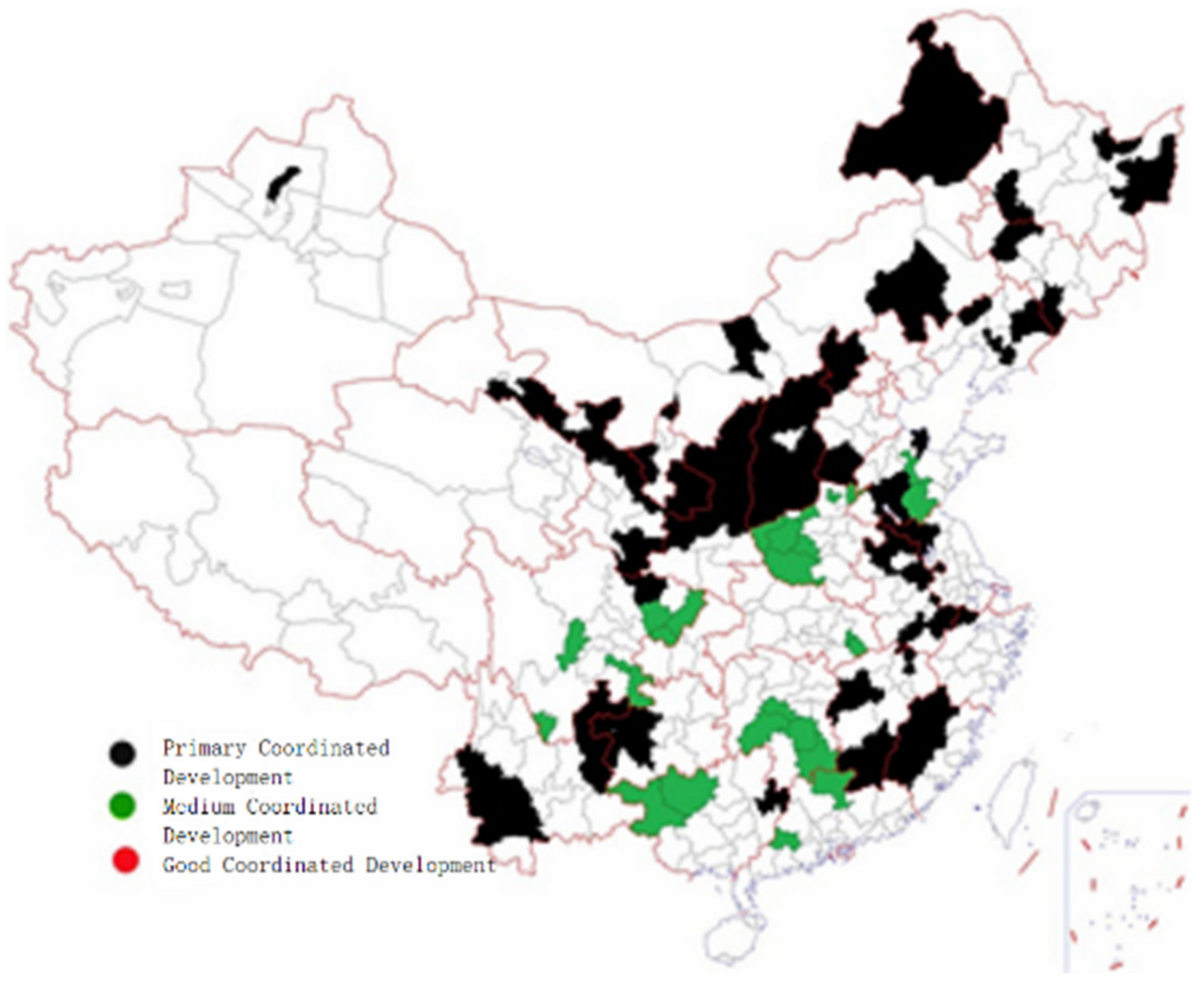
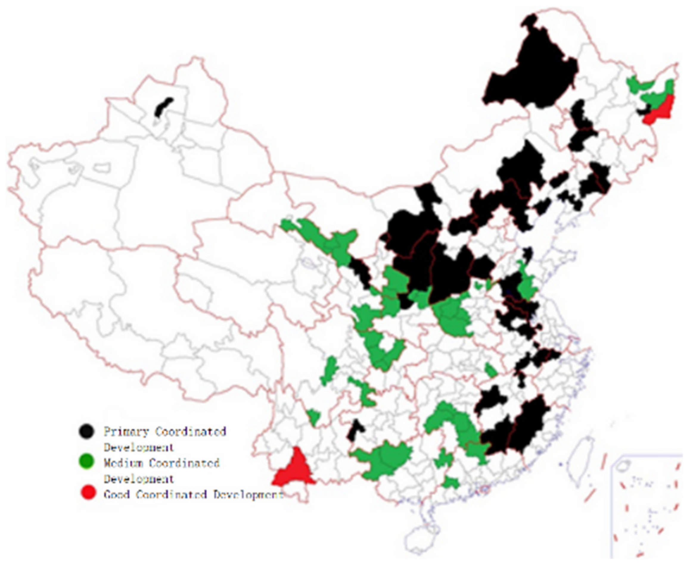
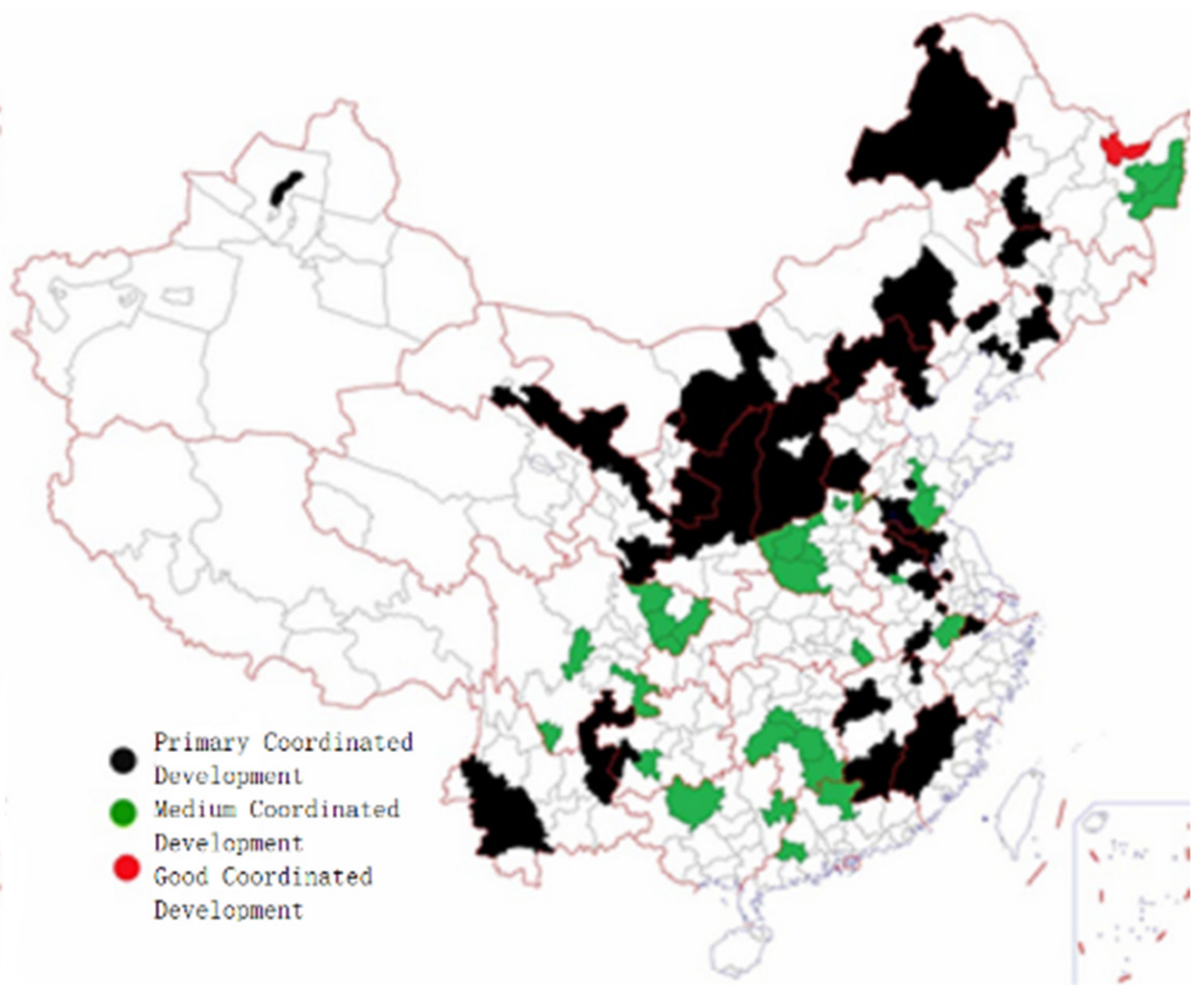
- The synergy between economy and environment in resource-based cities is not high that the environment lags behind obviously. It is easy to pay attention to that there are regional differences in coordination degree that the overall coordination of the eastern region is low, and the central and western regions show a high level.
- (4)
- The factors affecting the coordinated development of the economy and environment in resource-based cities are dense and obvious. The research results confirmed that indicators such as urban GDP, investment in fixed assets, and per capita solid waste discharge had played an important role in the coordinated development of resource-based cities’ economies and environment.
- (1)
- The government should improve the attractiveness of the urban manpower, provide complete welfare benefits for both the migrant workers and local workers, and improve the population quality of employees.
- (2)
- The government should enhance the urban industrial structure, increase the support for high value-added industries, strictly supervise pollution-intensive industries, encourage innovation and cultivate the high-tech industries.
- (3)
- While controlling environmental pollution and repairing ecological damage, the government should also pay attention to economic development to avoid economic weakness caused by excessive investment.
Author Contributions
Funding
Institutional Review Board Statement
Informed Consent Statement
Data Availability Statement
Acknowledgments
Conflicts of Interest
Appendix A

| Air Quality | Water | ||||
|---|---|---|---|---|---|
| 2009 | 2012 | 2015 | 2009 | 2012 | 2015 |
| 0.752059 | 0.750398 | 0.751473 | 0.289526 | 0.29062 | 0.289974 |
| 0.750005 | 0.749413 | 0.290727 | 0.29129 | ||
| 0.751075 | 0.751338 | 0.750163 | 0.290106 | 0.289962 | 0.290689 |
| 0.750823 | 0.752605 | 0.751276 | 0.290364 | 0.2893 | 0.290123 |
| 0.752365 | 0.751993 | 0.289383 | 0.289674 | ||
| 0.724623 | 0.752104 | 0.751947 | 0.30623 | 0.289602 | 0.289706 |
| 0.750048 | 0.747721 | 0.748388 | 0.29091 | 0.29236 | 0.291945 |
| 0.752203 | 0.751359 | 0.751143 | 0.289536 | 0.290058 | 0.290201 |
| 0.752061 | 0.750694 | 0.747788 | 0.289567 | 0.290456 | 0.292219 |
| 0.725015 | 0.71167 | 0.305689 | 0.314047 | ||
| 0.743917 | 0.751169 | 0.748413 | 0.294647 | 0.290189 | 0.291905 |
| 0.745091 | 0.713491 | 0.747473 | 0.293831 | 0.311648 | 0.292447 |
| 0.745985 | 0.751317 | 0.745874 | 0.29327 | 0.290062 | 0.293442 |
| 0.747701 | 0.751148 | 0.749932 | 0.292257 | 0.290213 | 0.290961 |
| 0.752295 | 0.753001 | 0.752215 | 0.289496 | 0.28906 | 0.289546 |
| 0.748528 | 0.749794 | 0.75073 | 0.291761 | 0.291025 | 0.290441 |
| 0.750457 | 0.753454 | 0.290646 | 0.288768 | ||
| 0.749232 | 0.752009 | 0.751407 | 0.291421 | 0.28967 | 0.290056 |
| 0.746994 | 0.745178 | 0.744518 | 0.292782 | 0.293887 | 0.29427 |
| 0.750292 | 0.750977 | 0.746678 | 0.290721 | 0.290301 | 0.292978 |
| 0.75157 | 0.752116 | 0.751162 | 0.289843 | 0.289566 | 0.290152 |
| 0.750995 | 0.748487 | 0.749936 | 0.290304 | 0.291803 | 0.290949 |
| 0.752608 | 0.751755 | 0.750742 | 0.289243 | 0.289812 | 0.290457 |
| 0.75258 | 0.749822 | 0.748414 | 0.289253 | 0.29097 | 0.291847 |
| 0.744473 | 0.74702 | 0.293846 | 0.292602 | ||
| 0.745638 | 0.749891 | 0.735022 | 0.293432 | 0.290891 | 0.299865 |
| 0.753088 | 0.752334 | 0.75019 | 0.288979 | 0.289154 | 0.29074 |
| 0.753357 | 0.752304 | 0.752089 | 0.288684 | 0.289385 | 0.28958 |
| 0.752442 | 0.289141 | ||||
| 0.752334 | 0.289413 | ||||
| 0.936888 | 0.749592 | 1.598564 | 0.235454 | 0.291022 | 0.401434 |
| 1.296465 | 0.753536 | 0.937323 | 0.454302 | 0.288647 | 0.358945 |
| 0.930656 | 0.75099 | 0.936639 | 0.238547 | 0.290217 | 0.359492 |
| 0.93699 | 0.75413 | 0.752522 | 0.235408 | 0.288308 | 0.289304 |
| 0.751847 | 0.75264 | 0.75254 | 0.289713 | 0.289232 | 0.289309 |
| 0.74527 | 0.744407 | 0.740109 | 0.292367 | 0.293936 | 0.296381 |
| 0.749836 | 0.7538 | 0.753547 | 0.290636 | 0.288476 | 0.288641 |
| 0.75288 | 0.751889 | 0.752272 | 0.288992 | 0.289636 | 0.289367 |
| 0.741561 | 0.727169 | 0.75335 | 0.290921 | 0.302729 | 0.288798 |
| 0.935246 | 0.753795 | 0.75335 | 0.3606 | 0.288524 | 0.288798 |
| 0.732686 | 0.752329 | 0.753722 | 0.293701 | 0.289316 | 0.288529 |
| 0.747844 | 0.750414 | 0.748822 | 0.292207 | 0.29063 | 0.291614 |
| 0.928764 | 0.753616 | 0.752609 | 0.363633 | 0.288619 | 0.289221 |
| 0.751559 | 0.751061 | 0.750308 | 0.289785 | 0.290174 | 0.290654 |
| 0.715748 | 0.74716 | 0.740155 | 0.307551 | 0.29264 | 0.29682 |
| 0.752677 | 0.752717 | 0.75318 | 0.289087 | 0.289184 | 0.288906 |
| 0.75361 | 0.752932 | 0.751516 | 0.28827 | 0.288802 | 0.289567 |
| 0.753069 | 0.753896 | 0.7534 | 0.288293 | 0.28837 | 0.288727 |
| 0.750448 | 0.754245 | 0.754371 | 0.290391 | 0.288262 | 0.288182 |
| 0.752834 | 0.697935 | 0.751357 | 0.288994 | 0.270997 | 0.289881 |
| 0.751559 | 0.751061 | 0.750308 | 0.289785 | 0.290174 | 0.290654 |
| 0.751622 | 0.67235 | 0.749614 | 0.289866 | 0.296012 | 0.291162 |
| 0.668151 | 0.75216 | 0.753039 | 0.315143 | 0.289361 | 0.288912 |
| 0.751686 | 0.752158 | 0.751656 | 0.289821 | 0.289532 | 0.289832 |
| 0.744411 | 0.743291 | 0.294121 | 0.294856 | ||
| 0.752477 | 0.752274 | 0.751341 | 0.289298 | 0.289436 | 0.290009 |
| 0.751553 | 0.747545 | 0.289893 | 0.292217 | ||
| 0.735343 | 0.751252 | 0.750921 | 0.299807 | 0.290148 | 0.290359 |
| 0.751599 | 0.753081 | 0.753069 | 0.289668 | 0.288953 | 0.28897 |
| 0.74937 | 0.75125 | 0.75143 | 0.29114 | 0.2901 | 0.28998 |
| 0.75215 | 0.75209 | 0.7513 | 0.28944 | 0.28956 | 0.29006 |
| 0.7471 | 0.75127 | 0.75132 | 0.29271 | 0.29009 | 0.29005 |
| 0.75324 | 0.752503 | 0.75151 | 0.28884 | 0.289294 | 0.28993 |
| 0.75296 | 0.752893 | 0.75152 | 0.28904 | 0.289099 | 0.28996 |
| 0.75171 | 0.75296 | 0.75258 | 0.28948 | 0.288981 | 0.28921 |
| 0.75319 | 0.753555 | 0.75328 | 0.28828 | 0.28859 | 0.28877 |
| 0.74992 | 0.753149 | 0.75178 | 0.29094 | 0.288949 | 0.28979 |
| 0.75329 | 0.750815 | 0.75311 | 0.28866 | 0.290301 | 0.28894 |
| 0.7356 | 0.752863 | 0.75108 | 0.29911 | 0.289118 | 0.29024 |
| 0.73765 | 0.742593 | 0.74688 | 0.2982 | 0.29539 | 0.29281 |
| 0.74844 | 0.752225 | 0.7429 | 0.29155 | 0.289421 | 0.29509 |
| 0.75203 | 0.75112 | 0.75049 | 0.28956 | 0.290135 | 0.29052 |
| 0.73473 | 0.748581 | 0.75024 | 0.29611 | 0.29148 | 0.29052 |
| 0.73506 | 0.736469 | 0.75162 | 0.29906 | 0.29842 | 0.28989 |
| 0.75261 | 0.738215 | 0.75106 | 0.28897 | 0.296927 | 0.29014 |
| 0.74569 | 0.749018 | 0.75336 | 0.29315 | 0.29129 | 0.28882 |
| 0.750542 | 0.75053 | 0.290497 | 0.29055 | ||
| 0.67594 | 0.730121 | 0.73277 | 0.3258 | 0.301652 | 0.30051 |
| 0.67728 | 0.752843 | 0.74458 | 0.32967 | 0.288908 | 0.29382 |
| 0.68896 | 0.676266 | 0.67061 | 0.31309 | 0.3236 | 0.32476 |
| 0.75135 | 0.748646 | 0.73671 | 0.28986 | 0.29168 | 0.29811 |
| 0.73034 | 0.753144 | 0.75152 | 0.30129 | 0.288964 | 0.28998 |
| 0.75037 | 0.752125 | 0.75192 | 0.29068 | 0.2896 | 0.28973 |
| 0.72803 | 0.746557 | 0.74852 | 0.30297 | 0.292822 | 0.29165 |
| 0.74928 | 0.751016 | 0.74959 | 0.29131 | 0.290261 | 0.29116 |
| 0.75048 | 0.752256 | 0.74982 | 0.29052 | 0.289529 | 0.29101 |
| 0.72087 | 0.752156 | 0.73337 | 0.30692 | 0.289547 | 0.30082 |
| 0.784468 | 0.784398 | 0.584707 | 0.230687 | 0.23071 | 0.501019 |
| 0.655221 | 0.658985 | 0.55386 | 0.352217 | 0.350143 | 0.329968 |
| 0.665189 | 0.829243 | 0.346387 | 0.364868 | ||
| 0.780499 | 0.785238 | 0.58558 | 0.232757 | 0.230276 | 0.458963 |
| 0.665401 | 0.654813 | 0.660048 | 0.345837 | 0.352474 | 0.358517 |
| 0.674493 | 0.626961 | 0.796009 | 0.338656 | 0.36906 | 0.345267 |
| 0.677786 | 0.670514 | 0.583785 | 0.338893 | 0.343146 | 0.333267 |
| 0.644091 | 0.670483 | 0.59196 | 0.359903 | 0.343376 | 0.093165 |
| 0.674382 | 0.654613 | 0.613681 | 0.341015 | 0.353041 | 0.382211 |
| 0.640081 | 0.582205 | 0.561135 | 0.35796 | 0.390625 | 0.303102 |
| 0.67144 | 0.659397 | 0.567867 | 0.339794 | 0.34897 | 0.377249 |
| 0.64932 | 0.596281 | 0.539441 | 0.35463 | 0.38792 | 0.402051 |
| 0.671199 | 0.675924 | 0.715323 | 0.342966 | 0.340035 | 0.321485 |
| 0.669892 | 0.674569 | 0.852626 | 0.343732 | 0.340859 | 0.308013 |
| 0.65813 | 0.660694 | 0.675472 | 0.350781 | 0.349264 | 0.329737 |
| 0.660462 | 0.669929 | 0.524097 | 0.349359 | 0.343698 | 0.361825 |
| 0.661404 | 0.666709 | 0.74041 | 0.348091 | 0.344668 | 0.315423 |
| 0.655905 | 0.636648 | 0.851786 | 0.350203 | 0.362707 | 0.305371 |
| 0.6436 | 0.676072 | 0.920043 | 0.359163 | 0.338628 | 0.338407 |
| 0.677044 | 0.677404 | 0.758067 | 0.339354 | 0.339129 | 0.360516 |
| 0.667373 | 0.674494 | 0.994378 | 0.345218 | 0.340879 | 0.222976 |
| 0.614518 | 0.65371 | 0.560969 | 0.376628 | 0.353616 | 0.343661 |
| 0.675398 | 0.674266 | 0.601362 | 0.339915 | 0.341025 | 0.18931 |
| Land | General environment | ||||
| 2009 | 2012 | 2015 | 2009 | 2012 | 2015 |
| 0.199678 | 0.200335 | 0.199835 | 0.413754 | 0.413784 | 0.413761 |
| 0.20068 | 0.200708 | 0.413804 | 0.413804 | ||
| 0.200155 | 0.200016 | 0.200539 | 0.413779 | 0.413772 | 0.413797 |
| 0.200142 | 0.1993 | 0.199893 | 0.413776 | 0.413735 | 0.413764 |
| 0.199487 | 0.199582 | 0.413745 | 0.413750 | ||
| 0.211798 | 0.199533 | 0.199593 | 0.414217 | 0.413746 | 0.413749 |
| 0.200409 | 0.201416 | 0.201126 | 0.413789 | 0.413832 | 0.413820 |
| 0.199496 | 0.199874 | 0.199959 | 0.413745 | 0.413764 | 0.413768 |
| 0.199629 | 0.200184 | 0.201504 | 0.413752 | 0.413778 | 0.413837 |
| 0.211892 | 0.216975 | 0.414199 | 0.414231 | ||
| 0.203179 | 0.199939 | 0.201134 | 0.413914 | 0.413766 | 0.413817 |
| 0.202795 | 0.214864 | 0.201592 | 0.413906 | 0.413334 | 0.413837 |
| 0.202373 | 0.199922 | 0.202255 | 0.413876 | 0.413767 | 0.413857 |
| 0.201584 | 0.199937 | 0.20049 | 0.413847 | 0.413766 | 0.413794 |
| 0.199435 | 0.199115 | 0.199466 | 0.413742 | 0.413725 | 0.413742 |
| 0.201179 | 0.20056 | 0.200159 | 0.413823 | 0.413793 | 0.413777 |
| 0.200241 | 0.198926 | 0.413781 | 0.413716 | ||
| 0.200763 | 0.199564 | 0.199816 | 0.413805 | 0.413748 | 0.413760 |
| 0.201755 | 0.202504 | 0.202776 | 0.413844 | 0.413856 | 0.413855 |
| 0.200344 | 0.200033 | 0.201887 | 0.413786 | 0.413770 | 0.413848 |
| 0.199879 | 0.199567 | 0.199996 | 0.413764 | 0.413750 | 0.413770 |
| 0.200014 | 0.201188 | 0.200496 | 0.413771 | 0.413826 | 0.413794 |
| 0.199364 | 0.199699 | 0.200131 | 0.413738 | 0.413755 | 0.413777 |
| 0.199385 | 0.200613 | 0.201234 | 0.413739 | 0.413802 | 0.413832 |
| 0.203471 | 0.201959 | 0.413930 | 0.413860 | ||
| 0.20258 | 0.200625 | 0.206711 | 0.413883 | 0.413802 | 0.413866 |
| 0.19911 | 0.199794 | 0.200452 | 0.413726 | 0.413761 | 0.413794 |
| 0.19914 | 0.199558 | 0.199579 | 0.413727 | 0.413749 | 0.413749 |
| 0.199684 | 0.413756 | ||||
| 0.199487 | 0.413745 | ||||
| 0.247724 | 0.200804 | 0.473355 | 0.413806 | 0.666666 | |
| 0.240965 | 0.198974 | 0.123781 | 0.663911 | 0.413719 | 0.473350 |
| 0.251177 | 0.200126 | 0.123955 | 0.473460 | 0.413778 | 0.473362 |
| 0.247661 | 0.19867 | 0.199394 | 0.473353 | 0.413703 | 0.413740 |
| 0.199705 | 0.199338 | 0.199363 | 0.413755 | 0.413737 | 0.413737 |
| 0.204289 | 0.203463 | 0.20559 | 0.413975 | 0.413935 | 0.414027 |
| 0.200981 | 0.198862 | 0.198966 | 0.413818 | 0.413713 | 0.413718 |
| 0.199341 | 0.199749 | 0.199614 | 0.413738 | 0.413758 | 0.413751 |
| 0.210056 | 0.212889 | 0.199011 | 0.414179 | 0.414262 | 0.413720 |
| 0.124312 | 0.19881 | 0.199011 | 0.473386 | 0.413710 | 0.413720 |
| 0.216766 | 0.199609 | 0.198892 | 0.414384 | 0.413751 | 0.413714 |
| 0.201478 | 0.200301 | 0.200993 | 0.413843 | 0.413782 | 0.413810 |
| 0.128571 | 0.198912 | 0.199391 | 0.473656 | 0.413716 | 0.413740 |
| 0.199959 | 0.200089 | 0.200412 | 0.413768 | 0.413775 | 0.413791 |
| 0.216946 | 0.201653 | 0.204555 | 0.413415 | 0.413818 | 0.413843 |
| 0.199467 | 0.199304 | 0.199087 | 0.413744 | 0.413735 | 0.413724 |
| 0.199328 | 0.199505 | 0.200275 | 0.413736 | 0.413746 | 0.413786 |
| 0.199944 | 0.198875 | 0.199039 | 0.413769 | 0.413714 | 0.413722 |
| 0.200545 | 0.198588 | 0.198534 | 0.413795 | 0.413698 | 0.413696 |
| 0.199389 | 0.277649 | 0.200083 | 0.413739 | 0.415527 | 0.413774 |
| 0.199959 | 0.200089 | 0.200412 | 0.413768 | 0.413775 | 0.413791 |
| 0.199788 | 0.279414 | 0.200629 | 0.413759 | 0.415925 | 0.413802 |
| 0.262742 | 0.199756 | 0.199249 | 0.415345 | 0.413759 | 0.413733 |
| 0.199768 | 0.199553 | 0.199792 | 0.413758 | 0.413748 | 0.413760 |
| 0.203074 | 0.203454 | 0.413869 | 0.413867 | ||
| 0.199453 | 0.199529 | 0.199943 | 0.413743 | 0.413746 | 0.413764 |
| 0.199833 | 0.201751 | 0.413760 | 0.413838 | ||
| 0.206816 | 0.199893 | 0.200035 | 0.413989 | 0.413764 | 0.413772 |
| 0.200053 | 0.199148 | 0.19914 | 0.413773 | 0.413727 | 0.413726 |
| 0.20093 | 0.19996 | 0.19988 | 0.413813 | 0.413770 | 0.413763 |
| 0.19967 | 0.1996 | 0.19994 | 0.413753 | 0.413750 | 0.413767 |
| 0.20271 | 0.199946 | 0.19992 | 0.414173 | 0.413769 | 0.413763 |
| 0.19909 | 0.199426 | 0.19984 | 0.413723 | 0.413741 | 0.413760 |
| 0.19919 | 0.199198 | 0.1998 | 0.413730 | 0.413730 | 0.413760 |
| 0.20015 | 0.199258 | 0.19943 | 0.413780 | 0.413733 | 0.413740 |
| 0.19982 | 0.199017 | 0.19913 | 0.413763 | 0.413721 | 0.413727 |
| 0.20053 | 0.19907 | 0.19969 | 0.413797 | 0.413723 | 0.413753 |
| 0.19925 | 0.200223 | 0.19913 | 0.413733 | 0.413780 | 0.413727 |
| 0.20758 | 0.199209 | 0.19999 | 0.414097 | 0.413730 | 0.413770 |
| 0.20592 | 0.203646 | 0.2018 | 0.413923 | 0.413876 | 0.413830 |
| 0.20156 | 0.199605 | 0.20381 | 0.413850 | 0.413750 | 0.413933 |
| 0.19967 | 0.200053 | 0.20033 | 0.413753 | 0.413769 | 0.413780 |
| 0.21186 | 0.201449 | 0.20065 | 0.414233 | 0.413837 | 0.413803 |
| 0.20814 | 0.206789 | 0.19977 | 0.414087 | 0.413893 | 0.413760 |
| 0.19969 | 0.206939 | 0.20012 | 0.413757 | 0.414027 | 0.413773 |
| 0.20285 | 0.201167 | 0.19898 | 0.413897 | 0.413825 | 0.413720 |
| 0.200315 | 0.20026 | 0.413785 | 0.413780 | ||
| 0.24172 | 0.209904 | 0.20851 | 0.414487 | 0.413892 | 0.413930 |
| 0.23536 | 0.199481 | 0.20325 | 0.414103 | 0.413744 | 0.413883 |
| 0.24245 | 0.243471 | 0.24818 | 0.414833 | 0.414446 | 0.414517 |
| 0.2001 | 0.201119 | 0.20612 | 0.413770 | 0.413815 | 0.413647 |
| 0.21048 | 0.199062 | 0.19978 | 0.414037 | 0.413723 | 0.413760 |
| 0.2003 | 0.199507 | 0.1996 | 0.413783 | 0.413744 | 0.413750 |
| 0.2112 | 0.202241 | 0.20134 | 0.414067 | 0.413873 | 0.413837 |
| 0.20082 | 0.200039 | 0.20066 | 0.413803 | 0.413772 | 0.413803 |
| 0.20035 | 0.19944 | 0.20057 | 0.413783 | 0.413742 | 0.413800 |
| 0.21373 | 0.199533 | 0.20792 | 0.413840 | 0.413745 | 0.414037 |
| 0.230685 | 0.230736 | 0.579895 | 0.415280 | 0.415281 | 0.555207 |
| 0.239119 | 0.237259 | 0.36414 | 0.415519 | 0.415462 | 0.415989 |
| 0.234602 | 0.232006 | 0.415393 | 0.475372 | ||
| 0.232763 | 0.230289 | 0.619636 | 0.415340 | 0.415268 | 0.554726 |
| 0.234896 | 0.239099 | 0.645392 | 0.415378 | 0.415462 | 0.554652 |
| 0.232661 | 0.250339 | 0.190266 | 0.415270 | 0.415453 | 0.443847 |
| 0.229001 | 0.232302 | 0.744881 | 0.415227 | 0.415321 | 0.553978 |
| 0.242506 | 0.232102 | 0.160135 | 0.415500 | 0.415320 | 0.281753 |
| 0.230421 | 0.238726 | 0.666623 | 0.415273 | 0.415460 | 0.554172 |
| 0.249221 | 0.275336 | 0.382737 | 0.415754 | 0.416055 | 0.415658 |
| 0.235029 | 0.238099 | 0.301732 | 0.415421 | 0.415489 | 0.415616 |
| 0.242902 | 0.263582 | 0.301732 | 0.415617 | 0.415928 | 0.414408 |
| 0.231771 | 0.229797 | 0.62704 | 0.415312 | 0.415252 | 0.554616 |
| 0.232358 | 0.230383 | 0.50325 | 0.415327 | 0.415270 | 0.554630 |
| 0.237412 | 0.236297 | 0.659474 | 0.415441 | 0.415418 | 0.554894 |
| 0.236494 | 0.232367 | 0.362078 | 0.415438 | 0.415331 | 0.416000 |
| 0.236778 | 0.234721 | 0.609103 | 0.415424 | 0.415366 | 0.554979 |
| 0.240345 | 0.247197 | 0.506695 | 0.415484 | 0.415517 | 0.554617 |
| 0.243752 | 0.231049 | 0.405707 | 0.415505 | 0.415250 | 0.554719 |
| 0.229312 | 0.229164 | 0.544434 | 0.415237 | 0.415232 | 0.554339 |
| 0.233477 | 0.23044 | 0.446197 | 0.415356 | 0.415271 | 0.554517 |
| 0.255959 | 0.239266 | 0.343402 | 0.415702 | 0.415531 | 0.416011 |
| 0.230463 | 0.230531 | 0.18931 | 0.415259 | 0.415274 | 0.326661 |
| The Current State of the City’s Economy | City Economic Power | General Economic Strength | ||||||
|---|---|---|---|---|---|---|---|---|
| 2009 | 2012 | 2015 | 2009 | 2012 | 2015 | 2009 | 2012 | 2015 |
| 0.080618 | 0.080612 | 0.080608 | 0.061024 | 0.061029 | 0.061032 | 0.708208 | 0.708205 | 0.708203 |
| 0.080627 | 0.080620 | 0.080612 | 0.061016 | 0.061022 | 0.061029 | 0.708212 | 0.708209 | 0.708205 |
| 0.080607 | 0.080607 | 0.080601 | 0.061033 | 0.061033 | 0.061038 | 0.708202 | 0.708202 | 0.708199 |
| 0.080602 | 0.080600 | 0.080596 | 0.061038 | 0.061039 | 0.061044 | 0.708200 | 0.708199 | 0.708196 |
| 0.080606 | 0.080607 | 0.080601 | 0.061034 | 0.061033 | 0.061039 | 0.708202 | 0.708202 | 0.708199 |
| 0.080636 | 0.080625 | 0.080617 | 0.061007 | 0.061017 | 0.061024 | 0.708217 | 0.708211 | 0.708208 |
| 0.080699 | 0.080718 | 0.080663 | 0.060951 | 0.060934 | 0.060983 | 0.708249 | 0.708258 | 0.708231 |
| 0.080644 | 0.080633 | 0.080613 | 0.061000 | 0.061010 | 0.061028 | 0.708221 | 0.708216 | 0.708205 |
| 0.080663 | 0.080654 | 0.080627 | 0.060983 | 0.060991 | 0.061016 | 0.708231 | 0.708226 | 0.708212 |
| 0.080631 | 0.080626 | 0.080612 | 0.061012 | 0.061017 | 0.061029 | 0.708215 | 0.708212 | 0.708205 |
| 0.080646 | 0.080633 | 0.080615 | 0.060999 | 0.061010 | 0.061026 | 0.708222 | 0.708215 | 0.708206 |
| 0.080637 | 0.080625 | 0.080609 | 0.061007 | 0.061017 | 0.061031 | 0.708218 | 0.708212 | 0.708203 |
| 0.080624 | 0.080617 | 0.080607 | 0.061019 | 0.061024 | 0.061033 | 0.708211 | 0.708208 | 0.708202 |
| 0.080644 | 0.080636 | 0.080612 | 0.061000 | 0.061007 | 0.061029 | 0.708221 | 0.708217 | 0.708205 |
| 0.080658 | 0.080651 | 0.080623 | 0.060988 | 0.060994 | 0.061020 | 0.708228 | 0.708225 | 0.708210 |
| 0.080638 | 0.080639 | 0.080643 | 0.061006 | 0.061005 | 0.061001 | 0.708218 | 0.708219 | 0.708221 |
| 0.080652 | 0.080642 | 0.080643 | 0.060993 | 0.061002 | 0.061001 | 0.708225 | 0.708220 | 0.708221 |
| 0.080891 | 0.080841 | 0.080813 | 0.060778 | 0.060822 | 0.060848 | 0.708341 | 0.708318 | 0.708305 |
| 0.080619 | 0.080613 | 0.080616 | 0.061022 | 0.061028 | 0.061025 | 0.708209 | 0.708205 | 0.708207 |
| 0.080633 | 0.080627 | 0.080628 | 0.061010 | 0.061015 | 0.061015 | 0.708216 | 0.708213 | 0.708213 |
| 0.080703 | 0.080667 | 0.080695 | 0.060948 | 0.060980 | 0.060954 | 0.708250 | 0.708232 | 0.708247 |
| 0.080673 | 0.080650 | 0.080755 | 0.060974 | 0.060995 | 0.060900 | 0.708236 | 0.708224 | 0.708277 |
| 0.080646 | 0.080641 | 0.080682 | 0.060998 | 0.061003 | 0.060966 | 0.708222 | 0.708219 | 0.708240 |
| 0.080636 | 0.080623 | 0.080625 | 0.061008 | 0.061019 | 0.061017 | 0.708217 | 0.708210 | 0.708212 |
| 0.080678 | 0.080665 | 0.080667 | 0.060969 | 0.060981 | 0.060979 | 0.708238 | 0.708232 | 0.708233 |
| 0.080668 | 0.080647 | 0.080774 | 0.060979 | 0.060997 | 0.060884 | 0.708233 | 0.708223 | 0.708286 |
| 0.080627 | 0.080638 | 0.080631 | 0.061016 | 0.061005 | 0.061012 | 0.708212 | 0.708218 | 0.708214 |
| 0.080655 | 0.080682 | 0.080684 | 0.060990 | 0.060966 | 0.060964 | 0.708227 | 0.708240 | 0.708242 |
| 0.080629 | 0.080641 | 0.080637 | 0.061014 | 0.061003 | 0.061006 | 0.708213 | 0.708219 | 0.708218 |
| 0.080580 | 0.080577 | 0.080672 | 0.061156 | 0.061158 | 0.061072 | 0.708680 | 0.708679 | 0.708723 |
| 0.080650 | 0.080614 | 0.080632 | 0.061093 | 0.061125 | 0.061109 | 0.708713 | 0.708697 | 0.708705 |
| 0.080678 | 0.080665 | 0.080826 | 0.061067 | 0.061079 | 0.060933 | 0.708726 | 0.708720 | 0.708793 |
| 0.080610 | 0.080581 | 0.080756 | 0.061129 | 0.061155 | 0.060996 | 0.708695 | 0.708681 | 0.708762 |
| 0.080692 | 0.080778 | 0.080806 | 0.061054 | 0.060976 | 0.060951 | 0.708732 | 0.708771 | 0.708784 |
| 0.080513 | 0.080512 | 0.080507 | 0.061217 | 0.061218 | 0.061222 | 0.708649 | 0.708649 | 0.708647 |
| 0.080506 | 0.080507 | 0.080504 | 0.061223 | 0.061223 | 0.061225 | 0.708646 | 0.708646 | 0.708645 |
| 0.080561 | 0.080557 | 0.080549 | 0.061174 | 0.061177 | 0.061184 | 0.708672 | 0.708670 | 0.708666 |
| 0.080544 | 0.080528 | 0.080522 | 0.061188 | 0.061203 | 0.061209 | 0.708664 | 0.708656 | 0.708653 |
| 0.080557 | 0.080550 | 0.080532 | 0.061177 | 0.061183 | 0.061200 | 0.708670 | 0.708667 | 0.708658 |
| 0.080581 | 0.080565 | 0.080535 | 0.061155 | 0.061170 | 0.061197 | 0.708681 | 0.708674 | 0.708660 |
| 0.080530 | 0.080531 | 0.080521 | 0.061201 | 0.061201 | 0.061210 | 0.708657 | 0.708658 | 0.708653 |
| 0.080578 | 0.080587 | 0.080558 | 0.061158 | 0.061150 | 0.061176 | 0.708680 | 0.708684 | 0.708670 |
| 0.080529 | 0.080541 | 0.080530 | 0.061203 | 0.061192 | 0.061202 | 0.708657 | 0.708662 | 0.708657 |
| 0.080537 | 0.080545 | 0.080539 | 0.061195 | 0.061188 | 0.061193 | 0.708661 | 0.708664 | 0.708662 |
| 0.080648 | 0.080634 | 0.080550 | 0.061095 | 0.061107 | 0.061184 | 0.708712 | 0.708706 | 0.708666 |
| 0.080585 | 0.080544 | 0.080527 | 0.061152 | 0.061189 | 0.061204 | 0.708683 | 0.708664 | 0.708656 |
| 0.080545 | 0.080541 | 0.080523 | 0.061188 | 0.061191 | 0.061208 | 0.708664 | 0.708663 | 0.708654 |
| 0.080543 | 0.080542 | 0.080526 | 0.061190 | 0.061190 | 0.061205 | 0.708663 | 0.708663 | 0.708655 |
| 0.080567 | 0.080549 | 0.080526 | 0.061168 | 0.061185 | 0.061205 | 0.708675 | 0.708666 | 0.708655 |
| 0.080573 | 0.080585 | 0.080564 | 0.061162 | 0.061151 | 0.061171 | 0.708678 | 0.708683 | 0.708673 |
| 0.080572 | 0.080591 | 0.080583 | 0.061163 | 0.061146 | 0.061154 | 0.708677 | 0.708686 | 0.708682 |
| 0.080545 | 0.080548 | 0.080542 | 0.061188 | 0.061185 | 0.061191 | 0.708664 | 0.708666 | 0.708663 |
| 0.080525 | 0.080518 | 0.080509 | 0.061206 | 0.061212 | 0.061221 | 0.708655 | 0.708652 | 0.708647 |
| 0.080529 | 0.080534 | 0.080515 | 0.061202 | 0.061198 | 0.061215 | 0.708657 | 0.708659 | 0.708650 |
| 0.080571 | 0.080556 | 0.080537 | 0.061164 | 0.061178 | 0.061195 | 0.708677 | 0.708669 | 0.708661 |
| 0.080523 | 0.080519 | 0.080510 | 0.061208 | 0.061212 | 0.061219 | 0.708654 | 0.708652 | 0.708648 |
| 0.080527 | 0.080520 | 0.080515 | 0.061204 | 0.061210 | 0.061215 | 0.708656 | 0.708653 | 0.708650 |
| 0.080641 | 0.080610 | 0.080574 | 0.061101 | 0.061129 | 0.061161 | 0.708709 | 0.708695 | 0.708678 |
| 0.080551 | 0.080539 | 0.080524 | 0.061182 | 0.061193 | 0.061206 | 0.708667 | 0.708661 | 0.708655 |
| 0.084989 | 0.084980 | 0.085968 | 0.080082 | 0.082091 | 0.080101 | 0.825357 | 0.835352 | 0.830345 |
| 0.084953 | 0.084950 | 0.084946 | 0.080114 | 0.080117 | 0.080120 | 0.825337 | 0.825335 | 0.825333 |
| 0.084992 | 0.084990 | 0.084971 | 0.080079 | 0.080082 | 0.080098 | 0.825359 | 0.825357 | 0.825347 |
| 0.085024 | 0.085018 | 0.085000 | 0.080051 | 0.080056 | 0.080073 | 0.825376 | 0.825373 | 0.825363 |
| 0.084975 | 0.084965 | 0.084956 | 0.080095 | 0.080103 | 0.080112 | 0.825349 | 0.825344 | 0.825338 |
| 0.084974 | 0.084974 | 0.084964 | 0.080096 | 0.080095 | 0.080105 | 0.825348 | 0.825349 | 0.825343 |
| 0.084979 | 0.084973 | 0.084963 | 0.080092 | 0.080097 | 0.080105 | 0.825351 | 0.825348 | 0.825342 |
| 0.084956 | 0.084955 | 0.084949 | 0.080111 | 0.080113 | 0.080117 | 0.825339 | 0.825338 | 0.825335 |
| 0.084950 | 0.084948 | 0.084945 | 0.080117 | 0.080119 | 0.080122 | 0.825335 | 0.825334 | 0.825332 |
| 0.085078 | 0.085056 | 0.085021 | 0.080003 | 0.080023 | 0.080054 | 0.825405 | 0.825393 | 0.825374 |
| 0.085004 | 0.084993 | 0.084972 | 0.080069 | 0.080079 | 0.080097 | 0.825365 | 0.825359 | 0.825347 |
| 0.084971 | 0.084966 | 0.084952 | 0.080098 | 0.080103 | 0.080116 | 0.825347 | 0.825344 | 0.825336 |
| 0.103809 | 0.085965 | 0.084955 | 0.061262 | 0.080104 | 0.080113 | 0.825357 | 0.830343 | 0.825338 |
| 0.084953 | 0.084954 | 0.086747 | 0.080114 | 0.080114 | 0.080119 | 0.825337 | 0.825337 | 0.834334 |
| 0.103819 | 0.084981 | 0.084965 | 0.061254 | 0.080090 | 0.080104 | 0.825364 | 0.825352 | 0.825344 |
| 0.103805 | 0.084998 | 0.084991 | 0.061266 | 0.080074 | 0.080080 | 0.825354 | 0.825361 | 0.825358 |
| 0.103813 | 0.084984 | 0.084972 | 0.061259 | 0.080087 | 0.080098 | 0.825360 | 0.825354 | 0.825347 |
| 0.103827 | 0.084958 | 0.084962 | 0.061247 | 0.080109 | 0.080107 | 0.825369 | 0.825340 | 0.825342 |
| 0.103835 | 0.085001 | 0.084980 | 0.061240 | 0.080072 | 0.080090 | 0.825375 | 0.825363 | 0.825352 |
| 0.103828 | 0.084972 | 0.084972 | 0.061246 | 0.070098 | 0.080097 | 0.825370 | 0.775347 | 0.825347 |
| 0.103831 | 0.084957 | 0.084953 | 0.061244 | 0.080111 | 0.080115 | 0.825372 | 0.825339 | 0.825336 |
| 0.103823 | 0.084972 | 0.084957 | 0.061250 | 0.080098 | 0.080111 | 0.825367 | 0.825347 | 0.825339 |
| 0.109950 | 0.084978 | 0.084978 | 0.055749 | 0.090093 | 0.080092 | 0.828496 | 0.875350 | 0.825350 |
| 0.103826 | 0.084980 | 0.084969 | 0.061247 | 0.080090 | 0.080100 | 0.825369 | 0.825352 | 0.825345 |
| 0.103807 | 0.085015 | 0.085003 | 0.061264 | 0.080060 | 0.080070 | 0.825356 | 0.825371 | 0.825365 |
| 0.103789 | 0.085069 | 0.085058 | 0.061279 | 0.080011 | 0.080021 | 0.825343 | 0.825400 | 0.825394 |
| 0.103825 | 0.084961 | 0.084955 | 0.061249 | 0.080107 | 0.080113 | 0.825368 | 0.825341 | 0.825338 |
| 0.103815 | 0.085018 | 0.085002 | 0.061257 | 0.080057 | 0.080071 | 0.825361 | 0.825372 | 0.825364 |
| 0.091552 | 0.090787 | 0.090295 | 0.050867 | 0.051746 | 0.052269 | 0.712095 | 0.712665 | 0.712820 |
| 0.090591 | 0.090168 | 0.089955 | 0.051958 | 0.052398 | 0.052609 | 0.712745 | 0.712830 | 0.712820 |
| 0.090094 | 0.089885 | 0.052471 | 0.052676 | 0.712825 | 0.712805 | |||
| 0.090098 | 0.089899 | 0.089848 | 0.052467 | 0.052663 | 0.052712 | 0.712825 | 0.712810 | 0.712800 |
| 0.091365 | 0.090684 | 0.090384 | 0.051089 | 0.051858 | 0.052176 | 0.712270 | 0.712710 | 0.712800 |
| 0.090746 | 0.090439 | 0.051792 | 0.052119 | 0.712690 | 0.712790 | |||
| 0.091673 | 0.090633 | 0.090302 | 0.050721 | 0.051914 | 0.052261 | 0.711970 | 0.712735 | 0.712815 |
| 0.090892 | 0.090379 | 0.090214 | 0.051631 | 0.052181 | 0.052350 | 0.712615 | 0.712800 | 0.712820 |
| 0.091928 | 0.091082 | 0.090709 | 0.050405 | 0.051417 | 0.051832 | 0.711665 | 0.712495 | 0.712705 |
| 0.090198 | 0.089933 | 0.089901 | 0.052367 | 0.052630 | 0.052611 | 0.712825 | 0.712815 | 0.712560 |
| 0.090097 | 0.089862 | 0.089715 | 0.052468 | 0.052698 | 0.052838 | 0.712825 | 0.712800 | 0.712765 |
| 0.089925 | 0.089736 | 0.089740 | 0.052638 | 0.052819 | 0.052815 | 0.712815 | 0.712775 | 0.712775 |
| 0.090263 | 0.089970 | 0.089800 | 0.052301 | 0.052593 | 0.052758 | 0.712820 | 0.712815 | 0.712790 |
| 0.090139 | 0.089906 | 0.089826 | 0.052426 | 0.052656 | 0.052733 | 0.712825 | 0.712810 | 0.712795 |
| 0.091581 | 0.091001 | 0.090727 | 0.050832 | 0.051509 | 0.051812 | 0.712065 | 0.712550 | 0.712695 |
| 0.091120 | 0.090584 | 0.090505 | 0.051374 | 0.051966 | 0.052050 | 0.712470 | 0.712750 | 0.712775 |
| 0.091575 | 0.090622 | 0.090301 | 0.050839 | 0.051925 | 0.052263 | 0.712070 | 0.712735 | 0.712820 |
References
- Li, W.; Yi, P. Assessment of city sustainability—Coupling coordinated development among economy, society and environment. J. Clean. Prod. 2020, 256, 120453. [Google Scholar] [CrossRef]
- Zhang, M.; Sun, X.; Wang, W. Study on the effect of environmental regulations and industrial structure on haze pollution in China from the dual perspective of independence and linkage. J. Clean. Prod. 2020, 256, 120748. [Google Scholar] [CrossRef]
- Wang, X.; Tian, G.; Yang, D.; Zhang, W.; Lu, D.; Liu, Z. Responses of PM2.5 pollution to urbanization in China. Energy Policy 2018, 123, 602–610. [Google Scholar] [CrossRef]
- Matsuyama, K. Agricultural productivity, comparative advantage, and economic growth. J. Econ. Theory 1992, 58, 317–334. [Google Scholar] [CrossRef] [Green Version]
- Auty, R. Sustaining Development in Mineral Economies: ‘The Resource Curse’ Thesis; Routledge: London, UK, 2002. [Google Scholar] [CrossRef]
- Jeffrey, D.; Saches, A.; Warner, M. Natural Resource Abundance and Economic Growth. Land Econ. 2005, 81, 496–502. [Google Scholar]
- Gylfason, T. Natural resources, education, and economic development. Eur. Econ. Rev. 2001, 45, 847–859. [Google Scholar] [CrossRef]
- Cole, M.A.; Neumayer, E. Examining the Impact of Demographic Factors on Air Pollution. Popul. Environ. 2004, 26, 5–21. [Google Scholar] [CrossRef] [Green Version]
- Larsen, E.R. Escaping the Resource Curse and the Dutch Disease? Am. J. Econ. Sociol. 2006, 65, 605–640. [Google Scholar] [CrossRef]
- Papyrakis, E.; Gerlagh, R. The resource curse hypothesis and its transmission channels. J. Comp. Econ. 2004, 32, 181–193. [Google Scholar] [CrossRef]
- Papyrakis, E.; Gerlagh, R. Resource abundance and economic growth in the United States. Eur. Econ. Rev. 2007, 51, 1011–1039. [Google Scholar] [CrossRef]
- Mikesell, R.F. Explaining the resource curse, with special reference to mineral-exporting countries. Resour. Policy 1997, 23, 191–199. [Google Scholar] [CrossRef]
- Wright, G. Resource-Based Growth Then and Now (Patterns of Integration in the Global Economy); ResearchGate: Berlin, Germany, 2001. [Google Scholar]
- Ginsburg, N. Natural Resource and Economic Development. Ann. Assoc. Am. Geogr. 1957, 47, 197–212. [Google Scholar] [CrossRef]
- Wen, M.; King, S.P. Push or pull? The relationship between development, trade and primary resource endowment. J. Econ. Behav. Organ. 2004, 53, 569–591. [Google Scholar] [CrossRef]
- Martin, W. Outgrowing Resource Dependence: Theory and Some Recent Developments. Int. Food Policy Res. Inst. 2005, 3482, 961–1027. [Google Scholar] [CrossRef]
- Boschini, A.D.; Pettersson, J.; Roine, J. Resource Curse or Not: A Question of Appropriability. Scand. J. Econ. 2007, 109, 593–617. [Google Scholar] [CrossRef] [Green Version]
- Same, A.T. Mineral-Rich Countries and Dutch Disease: Understanding the Macroeconomic Implications of Windfalls and The Development Prospects-The Case of Equatorial Guinea; World Bank: Washington, DC, USA, 2008; pp. 45–59. [Google Scholar] [CrossRef]
- Grossman, G.M.; Krueger, A.B. Environmental Impacts of a North American Free Trade Agreement; National Bureau of Economic Research: Cambridge, MA, USA, 1991. [Google Scholar] [CrossRef]
- Grossman, G.M.; Krueger, A.B. Economic growth and the environment. Q. J. Econ. 1995, 110, 353–377. [Google Scholar] [CrossRef] [Green Version]
- Spangenberg, J.H. The Environmental Kuznets Curve: A Methodological Artefact? Popul. Environ. 2001, 23, 175–191. [Google Scholar] [CrossRef]
- Wu, W.; Wang, W.; Zhang, M. Using China’s provincial panel data exploring the interaction between Socio-economic and Eco-environment system. Ecol. Complex. 2020, 44, 100873. [Google Scholar] [CrossRef]
- Xing, L.; Xue, M.; Hu, M. Dynamic simulation and assessment of the coupling coordination degree of the economy–resource–environment system: Case of Wuhan City in China. J. Environ. Manag. 2019, 230, 474–487. [Google Scholar] [CrossRef]
- Wang, Q.; Yuan, X.; Cheng, X.; Mu, R.; Zuo, J. Coordinated development of energy, economy and environment subsystems—A case study. Ecol. Indic. 2014, 46, 514–523. [Google Scholar] [CrossRef]
- Sun, Y.; Cui, Y. Analyzing the Coupling Coordination among Economic, Social, and Environmental Benefits of Urban Infrastructure: Case Study of Four Chinese Autonomous Municipalities. Math. Probl. Eng. 2018, 2018, 8280328. [Google Scholar] [CrossRef]
- Sun, Z.; Zhu, X.; Pan, Y.; Zhang, J.; Liu, X. Drought evaluation using the GRACE terrestrial water storage deficit over the Yangtze River Basin, China. Sci. Total Environ. 2018, 634, 727–738. [Google Scholar] [CrossRef]
- Deng, C.; Li, H.; Peng, D.; Liu, L.; Zhu, Q.; Li, C. Modelling the coupling evolution of the water environment and social economic system using PSO-SVM in the Yangtze River Economic Belt, China. Ecol. Indic. 2021, 129, 108012. [Google Scholar] [CrossRef]
- Srinivasan, V.; Seto, K.C.; Emerson, R.; Gorelick, S.M. The impact of urbanization on water vulnerability: A coupled human—Environment system approach for Chennai, India. Glob. Environ. Chang. 2013, 23, 229–239. [Google Scholar] [CrossRef]
- Fang, C.; Liu, H.; Li, G. International progress and evaluation on interactive coupling effects between urbanization and the eco-environment. J. Geogr. Sci. 2016, 26, 1081–1116. [Google Scholar] [CrossRef]
- Cheng, K.; He, K.; Fu, Q.; Tagawa, K.; Guo, X. Assessing the coordination of regional water and soil resources and ecological-environment system based on speed characteristics. J. Clean. Prod. 2022, 339, 130718. [Google Scholar] [CrossRef]
- Guan, D.; Gao, W.; Su, W.; Li, H.; Hokao, K. Modeling and dynamic assessment of urban economy–resource–environment system with a coupled system dynamics—Geographic information system model. Ecol. Indic. 2011, 11, 1333–1344. [Google Scholar] [CrossRef]
- Sauvé, S.; Bernard, S.; Sloan, P. Environmental sciences, sustainable development and circular economy: Alternative concepts for trans-disciplinary research. Environ. Dev. 2016, 17, 48–56. [Google Scholar] [CrossRef] [Green Version]
- Sunderland, T.; Butterworth, T. Meeting local economic decision-maker’s demand for environmental evidence: The Local Environment and Economic Development (LEED) toolkit. Ecosyst. Serv. 2016, 17, 197–207. [Google Scholar] [CrossRef] [Green Version]
- Zuo, Y.; Shi, Y.-L.; Zhang, Y.-Z. Research on the Sustainable Development of an Economic-Energy-Environment (3E) System Based on System Dynamics (SD): A Case Study of the Beijing-Tianjin-Hebei Region in China. Sustainability 2017, 9, 1727. [Google Scholar] [CrossRef] [Green Version]
- Estoque, R.C.; Murayama, Y. Social–ecological status index: A preliminary study of its structural composition and application. Ecol. Indic. 2014, 43, 183–194. [Google Scholar] [CrossRef]
- Kharazishvili, Y.; Kwilinski, A.; Grishnova, O.; Dzwigol, H. Social Safety of Society for Developing Countries to Meet Sustainable Development Standards: Indicators, Level, Strategic Benchmarks (with Calculations Based on the Case Study of Ukraine). Sustainability 2020, 12, 8953. [Google Scholar] [CrossRef]
- Yang, G.; Song, G.; Liu, H. The development of ecological environment in China based on the system dynamics method from the society, economy and environment perspective. J. Environ. Biol. 2016, 37, 155–162. [Google Scholar]
- Ning, X.L. Evaluation on coordination degree between environmental and economic development in Baotou city. J. Arid Land Resour. Environ. 2008, 22, 32–35. [Google Scholar]
- Fan, Y.; Fang, C.; Zhang, Q. Coupling coordinated development between social economy and ecological environment in Chinese provincial capital cities-assessment and policy implications. J. Clean. Prod. 2019, 229, 289–298. [Google Scholar] [CrossRef]
- Wang, Z.; Yuan, K.; Lu, C. Research on urban comprehensive carrying capacity based on resource and environmental Endowment and Pressure: A Case study of Dalian City. J. Arid Land Resour. Environ. 2015, 29, 64–69. [Google Scholar] [CrossRef]
- Guo, S.; Zhang, Y.; Huang, J. Coupling analysis of economy and environment of each city in Henan Province. Chin. Agric. Sci. Bull. 2016, 32, 193–198. [Google Scholar]
- Xu, N.; Yang, H.; Cheng, X.; Li, T. Spatial-temporal evolution pattern of coordination degree between economic strength and environmental carrying capacity in Shaanxi Province. Bull. Soil Water Conserv. 2017, 37, 152–158,166. [Google Scholar] [CrossRef]
- Shannon, C.E. The Mathematical Theory of Communication. BSTJ 1948, 27, 379–423. [Google Scholar] [CrossRef] [Green Version]

| For the ecological system | Ind(t) = 0 | Eco(t) = λC(t)/α(t) |
| Eco(t) = 0 | Ind(t) = λC(t) | |
| For the environmental ecosystem | Ind(t) = 0 | Eco(t) = ΦC(t) |
| Eco(t) = 0 | Ind(t) = ΦC(t)/β(t) |
| Definition | Value | Relationship |
|---|---|---|
| 1 | α(t) > 0 and β(t) > 0 | Competitive relationship |
| 2 | α(t) > 0 and β(t) < 0 | Favor symbiosis |
| 3 | α(t) < 0 and β(t) > 0 | / |
| 4 | α(t) < 0 and β(t) < 0 | Benign interaction |
| Classify | Relationship | Value |
|---|---|---|
| Symbiosis model | Mutually beneficial symbiosis model | α(t) < 0 and β(t) < 0 |
| Partial force symbiosis model | α(t) ≤ 0, β(t) ≤ 0 and α and β are not 0 at the same time | |
| Non-symbiotic model | Partial harm model | α(t) ≥ 0, β(t) ≥ 0 and α and β are not 0 at the same time |
| Single harm mode | α(t)β(t) < 0 | |
| Competitive model | α(t) > 0 and β(t) > 0 |
| Target Layer | Environmental Factors | Evaluation Index | Attributes |
|---|---|---|---|
| Comprehensive carrying capacity of resource-based cities | Air quality | Sulfur dioxide production [42] | − |
| Sulfur dioxide emissions | − | ||
| Industrial smoke (powder) dust removal | + | ||
| Industrial smoke (dust) emissions | − | ||
| Water | Industrial wastewater discharge | − | |
| Centralized treatment rate of sewage treatment plant | + | ||
| Land | Comprehensive utilization rate of general industrial solid waste | + | |
| Harmless treatment rate of domestic garbage | + |
| Target Layer | Environmental Factors | Evaluation Index | Attributes |
|---|---|---|---|
| The current state of the city’s economy | City GDP | GDP per capita | + |
| Economic growth rate | Annual economic growth rate | + | |
| Proportion of added value by industry | Proportion of secondary industry | + | |
| The proportion of tertiary industry | + | ||
| Disposable Personal income | Per capita disposable income | + | |
| The Driving force of City economy | Investment in fixed assets | Total investment in fixed assets | + |
| Unemployment rate | Urban unemployment rate | − | |
| Urban public service level | Public Finance Expenditure | + | |
| Science and technology | Science and Technology Expenditure | + |
| The-First Level | The-Second Level | Contrast Relationship | Types |
|---|---|---|---|
| (0.90, 1.00) | High-qualitied coordinated development | Economic lag | |
| Environmental and economic synchronous | |||
| Environmental lag | |||
| Economic lag | |||
| (0.80, 0.90) | Good coordinated development | Environmental and economic synchronous | |
| Environmental lag | |||
| Economic lag | |||
| (0.70, 0.80) | Medium coordinated development | Environmental and economic synchronous | |
| Environmental lag | |||
| Economic lag | |||
| (0.60, 0.70) | Primary coordinated development | Environmental and Economic synchronous | |
| Environmental lag | |||
| Economic lag | |||
| (0.50, 0.60) | Barely coordinated development | Environmental and Economic synchronous | |
| Enviromental lag | |||
| Economic lag | |||
| (0.40, 0.50) | Maladjustment on the verge of decline | Environmental and Economic synchronous | |
| Environmental lag | |||
| Economic lag | |||
| (0.30, 0.40) | Mild maladjustment recession | Environmental and Economic synchronous | |
| Environmental lag | |||
| Economic lag | |||
| [0.20, 0.30) | Moderate maladjusted recession | Environmental and Economic synchronous | |
| Environmental lag | |||
| Economic lag | |||
| (0.10, 0.20) | Severe maladjustment recession | Environmental and Economic synchronous | |
| Environmental lag | |||
| Economic lag | |||
| (0, 0.10) | Extreme maladjustment recession | Envirronmetal and Economic synchronous | |
| Environmental lag |
| Variables | Max | Min | Average | Standard Error | Observed Value |
|---|---|---|---|---|---|
| Coupling coordination degree | 0.745 | 0.520 | 0.589 | 0.036 | 109 |
| GDP | 6103.060 | 0.000 | 1411.806 | 1096.197 | 109 |
| GDP per capita | 20.716 | 0.000 | 4.013 | 3.304 | 109 |
| Annual average population (the whole city) | 1186.310 | 39.560 | 369.914 | 251.278 | 109 |
| Average annual population (municipal district) | 332.070 | 22.680 | 97.797 | 61.785 | 109 |
| The population density | 1024.360 | 10.250 | 341.281 | 256.900 | 109 |
| The proportion of secondary industry in GDP | 0.715 | 0.000 | 0.417 | 0.197 | 109 |
| The balance of various RMB deposits of financial institutions at the end of the year | 7456.807 | 324.588 | 1655.585 | 1122.796 | 109 |
| Balance of various RMB loans of financial institutions at the end of the year | 9027.592 | 145.846 | 1147.186 | 1081.190 | 109 |
| Public finance expenditure | 752.460 | 52.173 | 258.843 | 136.280 | 109 |
| Science and technology expenditure | 86.835 | 0.000 | 3.377 | 8.576 | 109 |
| Education expenditure | 152.350 | 7.139 | 46.393 | 28.266 | 109 |
| Practitioners in the secondary industry | 61.914 | 1.900 | 16.420 | 12.091 | 109 |
| Practitioners in the construction industry | 30.037 | 0.000 | 4.531 | 5.254 | 109 |
| Amount of foreign capital actually used in the year | 25.537 | 0.000 | 3.305 | 4.582 | 109 |
| Investment in fixed assets | 4543.877 | 0.000 | 1191.406 | 1012.983 | 109 |
| Industrial wastewater discharge | 712,158.0 | 0.000 | 12,493.340 | 69,285.150 | 109 |
| Industrial sulfur dioxide production | 212.346 | 0.000 | 23.561 | 30.100 | 109 |
| Industrial sulfur dioxide emissions | 22.553 | 0.000 | 5.480 | 4.828 | 109 |
| Industrial smoke (powder) dust removal | 1471.849 | 0.776 | 271.919 | 239.069 | 109 |
| Industrial smoke (dust) emissions | 46.690 | 0.431 | 4.798 | 5.829 | 109 |
| Comprehensive utilization rate of general industrial solid waste | 1.000 | 0.000 | 0.775 | 0.254 | 109 |
| Centralized treatment rate of sewage treatment plant | 1.000 | 0.000 | 0.865 | 0.136 | 109 |
| Harmless treatment rate of domestic garbage | 1.000 | 0.000 | 0.902 | 0.201 | 109 |
| Years | Air quality | Water | Land | General Environment |
|---|---|---|---|---|
| 2009 | 0.7095429 | 0.314384 | 0.2197904 | 0.41457244 |
| 2012 | 0.7292113 | 0.3023484 | 0.2109992 | 0.41418629 |
| 2015 | 0.75295 | 0.31154 | 0.2624 | 0.441495 |
| Carrying capacity level | Medium to high carrying capacity | Low to medium carrying capacity | Low to medium carrying capacity | Medium capacity |
| City Types | Air Quality | Water | Land | Overall Environmental Carrying Capacity |
|---|---|---|---|---|
| Growing city | 0.7585 | 0.30718 | 0.30096 | 0.455547 |
| Mature city | 0.75794 | 0.30115 | 0.25381 | 0.436198 |
| Declining city | 0.74118 | 0.30779 | 0.23005 | 0.426341 |
| Regenerative city | 0.74361 | 0.29423 | 0.2338 | 0.423879 |
| Years | The Current State of the City’s Economy | City Economic Power | General Economic Strength |
|---|---|---|---|
| 2009 | 0.86350452 | 0.61556952 | 0.739537019 |
| 2012 | 0.83733099 | 0.64113436 | 0.739232671 |
| 2015 | 0.83714836 | 0.6413114 | 0.739229877 |
| Evaluation grade | High capacity | Medium to high carrying capacity | Medium to high carrying capacity |
| Influencing Factors | Coefficient | p-Value |
|---|---|---|
| GDP | 0.3522 | 0.1650 |
| GDP per capita | −0.0405 | 0.8280 |
| Annual average population (the whole city) | 0.3260 * | 0.0870 |
| Average annual population (municipal district) | −0.0904 | 0.4590 |
| The population density | 0.0400 | 0.6270 |
| The proportion of secondary industry in GDP | −0.1840 ** | 0.0230 |
| The balance of various RMB deposits of financial institutions at the end of the year | −0.1851 | 0.4560 |
| Balance of various RMB loans of financial institutions at the end of the year | −0.0033 | 0.9840 |
| Public finance expenditure | −0.1421 | 0.5530 |
| Science and technology expenditure | −0.0777 | 0.5980 |
| Education expenditure | −0.0715 | 0.7570 |
| Practitioners in the secondary industry | −0.1028 | 0.5820 |
| Practitioners in the construction industry | 0.2438 | 0.1400 |
| Amount of foreign capital actually used in the year | 0.1126 | 0.2570 |
| Investment in fixed assets | −0.3800 ** | 0.0190 |
| Constant term | 0.4284 *** | 0.0000 |
| Influencing Factors | Coefficient | p-Value |
|---|---|---|
| Industrial wastewater discharge | 0.3018 * | 0.0560 |
| Industrial sulfur dioxide production | −0.0687 | 0.5340 |
| Industrial sulfur dioxide emissions | 0.0238 | 0.8000 |
| Industrial smoke (powder) dust removal | −0.0987 | 0.4960 |
| Industrial smoke (dust) emissions | −0.2405 | 0.1200 |
| Comprehensive utilization rate of general industrial solid waste | −0.1153 * | 0.0530 |
| Centralized treatment rate of sewage treatment plant | −0.2499 | 0.0340 |
| Harmless treatment rate of domestic garbage | −0.0450 | 0.5510 |
| Constant term | 0.6910 *** | 0.0000 |
| Influencing Factors | Coefficient | p-Value |
|---|---|---|
| GDP | 0.0915 | 0.7740 |
| GDP per capita | 0.4558 | 0.1950 |
| Annual average population (the whole city) | 0.5184 | 0.1410 |
| Average annual population (municipal district) | −0.3654 ** | 0.0410 |
| The population density | 0.0825 | 0.5430 |
| The proportion of secondary industry in GDP | −0.2310 ** | 0.0870 |
| The balance of various RMB deposits of financial institutions at the end of the year | −0.8948 | 0.0360 |
| Balance of various RMB loans of financial institutions at the end of the year | 0.1159 | 0.5260 |
| Public finance expenditure | 0.6129 | 0.2430 |
| Science and technology expenditure | −0.2634 | 0.2060 |
| Education expenditure | −0.6494 | 0.1750 |
| Practitioners in the secondary industry | 0.0982 | 0.7270 |
| Practitioners in the construction industry | 0.2423 | 0.4330 |
| Amount of foreign capital actually used in the year | −0.0595 | 0.7230 |
| Investment in fixed assets | −0.4462 * | 0.0750 |
| Constant term | 0.4817 *** | 0.0000 |
| Influencing Factors | Coefficient | p-Value |
|---|---|---|
| Industrial wastewater discharge | 0.4206 ** | 0.0160 |
| Industrial sulfur dioxide production | −0.0312 | 0.8630 |
| Industrial sulfur dioxide emissions | 0.2349 * | 0.0660 |
| Industrial smoke (powder) dust removal | −0.3004 | 0.1630 |
| Industrial smoke (dust) emissions | −0.5335 ** | 0.0300 |
| Comprehensive utilization rate of general industrial solid waste | −0.0858 | 0.2680 |
| Centralized treatment rate of sewage treatment plant | −0.4301 * | 0.0130 |
| Harmless treatment rate of domestic garbage | 0.0809 | 0.6240 |
| Constant term | 0.7213 *** | 0.0000 |
Publisher’s Note: MDPI stays neutral with regard to jurisdictional claims in published maps and institutional affiliations. |
© 2022 by the authors. Licensee MDPI, Basel, Switzerland. This article is an open access article distributed under the terms and conditions of the Creative Commons Attribution (CC BY) license (https://creativecommons.org/licenses/by/4.0/).
Share and Cite
Li, Q.; Guo, Q.; Zhou, M.; Xia, Q.; Quan, M. Analysis on the Mechanism and Influencing Factors of the Coordinated Development of Economy and Environment in China’s Resource-Based Cities. Sustainability 2022, 14, 2929. https://doi.org/10.3390/su14052929
Li Q, Guo Q, Zhou M, Xia Q, Quan M. Analysis on the Mechanism and Influencing Factors of the Coordinated Development of Economy and Environment in China’s Resource-Based Cities. Sustainability. 2022; 14(5):2929. https://doi.org/10.3390/su14052929
Chicago/Turabian StyleLi, Quan, Quan Guo, Min Zhou, Qing Xia, and Mengqi Quan. 2022. "Analysis on the Mechanism and Influencing Factors of the Coordinated Development of Economy and Environment in China’s Resource-Based Cities" Sustainability 14, no. 5: 2929. https://doi.org/10.3390/su14052929
APA StyleLi, Q., Guo, Q., Zhou, M., Xia, Q., & Quan, M. (2022). Analysis on the Mechanism and Influencing Factors of the Coordinated Development of Economy and Environment in China’s Resource-Based Cities. Sustainability, 14(5), 2929. https://doi.org/10.3390/su14052929