Towards Maximizing Hosting Capacity by Optimal Planning of Active and Reactive Power Compensators and Voltage Regulators: Case Study

Abstract

Improving the performance of distribution systems is one of the main objectives of power system operators. This can be done in several ways, such as network reconfiguration, system reinforcement, and the addition of different types of equipment, such as distributed generation (DG) units, shunt capacitor banks (CBs), and voltage regulators (VRs). In addition, the optimal use of renewable and sustainable energy sources (RSESs) has become crucial for meeting the increase in demand for electricity and reducing greenhouse gas emissions. This requires the development of techno-economic planning models that can measure to what extent modern power systems can host RSESs. This article applies a new optimization technique called RUN to increase hosting capacity (HC) for a rural Egyptian radial feeder system called the Egyptian Talla system (ETS). RUN relies on mathematical concepts and principles of the widely known Runge–Kutta (RK) method to get optimal locations and sizes of DGs, CBs, and VRs. Furthermore, this paper presents a cost-benefit analysis that includes fixed and operating costs of the compensators (DGs, CBs, and VRs), the benefits obtained by reducing the power purchased from the utility, and the active power loss. The current requirements of Egyptian electricity distribution companies are met in the formulated optimization problem to improve the HC of this rural system. Uncertain loading conditions are taken into account in this study. The main load demand clusters are obtained using the soft fuzzy C-means clustering approach according to load consumption patterns in this rural area. The introduced RUN optimization algorithm is used to solve the optimal coordination problem between DGs, CBs, and VRs. Excellent outcomes are obtained with a noteworthy reduction in the distribution network power losses, improvement in the system’s minimum voltage, and improvement of the loading capacity. Several case studies are investigated, and the results prove the efficiency of the introduced RUN-based methodology, in which the probabilistic HC of the system reaches 100% when allowing reverse power flow to the utility. In comparison, this becomes 49% when allowing reverse power to flow back to the utility.

1. Introduction

In 2022, renewable energy growth is accelerating as interest in climate change increases, in line with augmented technical, environmental, and social considerations and governance support. In this context, the demand for cleaner energy sources from most market sectors is accelerating. Fortunately, the penetration of renewable energy resources in radial distribution systems (RDSs) helps improve the performance of these systems [1,2]. Optimal allocation (i.e., location and size) of multiple centralized/decentralized renewable energy resources at different buses of the system can give numerous benefits [3], such as reducing the system power losses and peak power requirements, boosting the voltage profile, ancillary services provisioning, deferring the upgrading process of distribution system lines/cables, and enhancing the system reliability [4,5]. Moreover, reactive power compensators such as capacitor banks (CBs), series compensators, shunt reactors, static VAR compensators (SVCs) [6], static synchronous compensators, and synchronous condensers can be added to these systems to enhance the voltage profile of nodes and improve the power factor of loads [7]. Voltage regulators (VRs) can also be an efficient solution to minimize voltage deviations in RDSs. The recent VR technologies provide significant advantages over traditional VR designs—electronic control with more advanced features to support innovative grid technologies and quick-drive tap changers that operate within only 10 s through 32 steps; this allows fast recovery from large voltage swings and power quality improvement.

Unfortunately, non-optimal integration of renewables and reactive power compensators may increase power system losses and cause thermal overloading and overvoltage problems, weaken systems’ power quality (PQ) and reliability [8], and trigger harmonic distortion problems by inverter-based distributed generation units, especially if feeding nonlinear loads.

Several studies have been conducted to solve these problems by quantifying the proper penetration of renewables in hosting capacity (HC) analysis frameworks. HC is an indicator for network operators of the available renewable capabilities, so that the power system can effectively make the best use of them. The HC border in the distribution network is an easy-to-calculate indicator, on scientific but reliable grounds, to decide where and when more renewables can be added to the system without surpassing the operational constraints [9,10]. In this context, several actions can enhance the HC of a system, such as (i) voltage control using on-load tap changers (OLTCs), which is considered an efficient way to control voltage profiles; (ii) reactive power control, which is regarded as one of the most efficient solutions to solve reactive power and voltage problems by adding external compensators such as CBs, static VAR compensators (SVCs), and others; (iii) active power control, in which active power curtailment techniques can be applied in centralized renewables-based power stations to control their output power by balancing the mismatch between power generation and consumption; and (iv) using energy storage systems to overcome the overvoltage problems from the high penetration of renewables. The proper planning of energy storage units can postpone the upgrading process of modern distribution systems: (v) reinforcing and/or reconfiguring power system networks in planning stages can also accommodate high HC levels, and (vi) harmonic management can be used to minimize harmonic distortion, as the nonlinearity degree of loads can impact the targeted HC level. It should be mentioned that more than one solution can be applied to make the best use of renewables and to get the highest possible HC.

Distribution networks connect high-voltage transmission systems to low-voltage customers. RDSs have a simple design and construction and cheap cost advantages. Load growth in RDSs has a detrimental influence on power system quality, resulting in increased voltage variations, feeder overloading (increased values of branch currents), and increased power loss in systems not ready for it. Simultaneous allocation of distributed generation (DG) units, VRs, and reactive compensators can be an efficient solution to enhance the PQ of these deteriorated RDSs. In this regard, few studies have examined the optimal allocation of DGs, CBs, and VRs for maximizing the HC of deteriorated RDSs.

Many research studies have been conducted to allocate DGs and CBs simultaneously in RDSs in the literature [11,12,13,14]. In [11], the authors identified appropriate DG and CB locations, sizes, and types for small, isolated networks with nonlinear loads at the planning phase. In [12], the Manta ray foraging optimization technique manages the DGs and CBs allocation in RDSs for reducing energy loss using appropriate data to meet customer expectations. The firefly and backtracking optimization techniques were used in [14] to solve the optimal coordination issue for DGs and CBs in RDSs for reducing power loss and enhancing the voltage magnitude of all buses. In [13], the authors suggested a multiobjective model with a two-stage fuzzy approach based on the grasshopper optimization algorithm for optimum allocation of DGs, CBs, and EV charging stations, while considering various technical PQ performance indicators.

Additionally, the problem of optimal coordination between DGs and VRs was addressed in [15,16,17] to decrease system losses, control and improve the voltage profile, and enhance voltage stability. In addition, the authors of [18] discussed using multi-agents (DGs, CBS/SVC, or VRs) to improve the performance of RDSs, while considering various PQ indices. However, HC analysis was not conducted in detail.

This article applies a new optimization technique to obtain optimal locations and sizes of DGs, CBs, and VRs to increase HC for a rural Egyptian radial feeder system called the Egyptian Talla system (ETS). A recently introduced RUN optimization technique is used to solve the desired allocation problem in two cases. The first case considers reverse power flow to the utility, while the second prevents reverse power flow in the feeder. RUN relies on mathematical concepts and principles of the widely known Runge–Kutta (RK) method. Furthermore, this paper presents a cost-benefit analysis (CBA) that includes fixed and operating costs of the compensators (DGs, CBs, and VRs) and the benefits obtained by enhancing the voltage stability of the system and reducing the active power loss, voltage deviation, loading capacity, and power purchased from the utility. The CBA can measure the benefits of a particular action for system operators and customers minus the costs of taking that action.

In addition, the current requirements of Egyptian electricity distribution companies were met in the formulated optimization problem to improve the HC of this rural system. Uncertain loading conditions were taken into account in this study. The main load demand clusters were obtained using the soft fuzzy C-means clustering approach according to load consumption patterns in this system.

The core contributions of this article are summarized in the following points:

• A new optimization methodology is applied to obtain the optimal allocation of various units (DGs, CBs, and VRs) to maximize the HC in a real deteriorated Egyptian system, while taking into consideration load demand uncertainty.
• A probabilistic HC planning model is proposed, increasing renewables penetration and meeting load demands in the studied system.
• A CBA is introduced, considering the costs of all compensators (DGs, CBs, and VRs) and the benefits of decreasing the power losses and the total power purchased from the utility.
• The simulation results validate the efficiency of solving the simultaneous allocation problem of DGs, CBs, and VRs, while complying with the considered linear and nonlinear constraints in an efficient techno-economical manner.
• The simulation results show the proposed strategy’s efficiency in solving the optimal sizing and siting problem cost-effectively. The probabilistic HC of the system reaches 100% when allowing a reverse power flow to the utility. In comparison, this becomes 49% when not allowing the reverse power to flow back to the utility.

The rest of the paper is arranged as follows: Section 2 presents an overview of recent related HC studies. Section 3 illustrates the VR model and optimal load flow. Section 4 explains the system under study, the problem formulation, and the RUN optimization algorithm employed. Section 5 presents the obtained simulation results and their discussion. The conclusions derived from this study are provided in Section 6.

2. Related Works

The terminology “hosting capacity” (HC) is a relatively new concept that refers to the maximum penetration of DGs that a system can host without operational problems [19,20,21]. Figure 1 illustrates HC calculation using a generic performance index versus penetration level. The performance index is determined based on the issue in the power network.

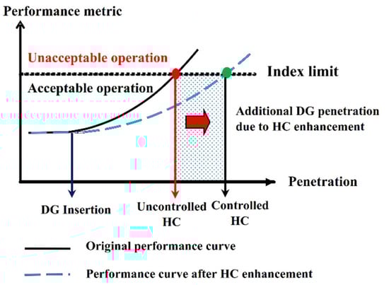
Figure 1. HC demonstration using a general performance index.

Figure 2 shows the typical operational problems and HC enhancement solutions in modern RDSs. In the near past, conventional rules of thumb were used to decide on adding renewables. However, they were not widely used as the HC definition. Nowadays, HC determination can assess the addition of renewables reasonably. HC has been embedded in several well-known simulation software applications due to its importance, such as DIGSilent, CYME, EPRI (DRIVE), ETAP, and Siemens, as shown in Table 1. The reader can refer to [19,20,21] for more details about HC calculation.

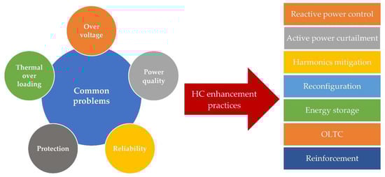
Figure 2. Common problems and HC enhancement practices.

Table 1. HC determination in the well-known simulation software.

Software	Name	Description
	DIGSilent	DIGSilent offers features to solve the DG problems, such as the reverse flow and the increase in the system voltage. A built-in interface determines the HC, relying on SCADA system measurements.
	CYME	Network HC can be determined by connecting one DG or more than one without exceeding the operational constraints.
	EPRI Drive Module	This module decides the maximum HC of the distribution system in its current state before exceeding system constraints such as reliability, protection, and PQ issues.
	ETAP	Maximum HC can be calculated by performing the worst-case scenario load flow analysis to identify renewables’ negative impacts on the distribution system’s performance.
	Siemens	The new capacity module has the potential to obtain the maximum HC at each distribution system point without exceeding the operational constraints.

SVCs were optimally designed using multi-stage stochastic optimization to allocate photovoltaic (PV) units [22]. An appropriately sized C-type harmonic filter enhanced the HC of a system operating under non-sinusoidal conditions in [23]. In [24], HC was analyzed for an 18-node practical distribution feeder using a decoupled harmonic power flow model, and it was found that by decentralizing the DG capacity, higher penetration levels could be obtained. In [25], the authors examined the influence of autonomous voltage control techniques on the PV-HC in LV distribution feeders. The operating strategies explored were based on the PV systems’ active and reactive power control capabilities and the capability of OLTCs. The authors of [26] examined the effect of reactive power management of the PV inverter on the PV-based HC of a distribution network. When a DG unit’s output power exceeds the load requirement, the excess electricity is returned to the grid. As a result, a voltage rise at the load bus may occur, potentially resulting in an overload at the adjacent feeder. In addition, the effects of tap locations of OLTCs and SVCs configurations were investigated.

Uncertainties of generation, load demand, and renewables are challenging to model and risky to manage in a deterministic way. The main difficulty is determining the appropriate solutions for calculating deviations of these parameters from their nominal values. The authors of [10] proposed an HC maximization approach considering different technical constraints, such as power flow equations and feeders’ maximum allowable voltages and currents, and economic conditions, such as the cost of energy procurement from the upstream network and power generation by renewable energy sources. The authors presented a stochastic multi-objective optimization model to maximize the HC and minimize the energy procurement costs in a power system integrated with wind systems. Shayani et al. [27] evaluated the influence of high PV penetration on electrical networks. The authors discovered that when DG penetration is substantial, the voltage rise and the continuous conductor maximum current are the primary indices that exceed the permitted limits. The authors concluded from their calculations that installing DG level between 1 and 2 p.u of the load power could be possible.

The authors of [28] provided an approach in which a multi-objective and multi-period optimization model was formulated, where the demand response is utilized as an effective tool to increase HC and decrease energy losses simultaneously. The authors of [29] developed a multi-objective bilevel optimization problem to optimize the HC that meets distribution system reconfiguration (DSR) and placement of soft opening points (SOP) for two real distribution systems, one with 59 nodes in Egypt and another with 83 nodes in Taiwan. The outcomes demonstrated the efficacy of DSR and SOP allocation to optimize the HC of the distribution systems. The authors of [30] proposed a maximum HC evaluation method, while considering the robust optimal operation of OLTCs and SVCs, as well as the uncertainty of DG power outputs and load demands. An actual 55-bus rural feeder in China was modeled to demonstrate the advantages of the proposed technique over the standard method and validate the value in PV-planning decision making for utilities. The sensitivity of interval-valued PV-HC to the number of Monte Carlo simulations was investigated. In this regard, uncertainty analysis has gained much attention in these works [31,32]. In [33], a stochastic optimization was devised for the best position of SVCs to enhance the penetration of solar PV energy, while accounting for renewables and load uncertainty.

The authors of [34] introduced an enhanced grey wolf algorithm (EGWA) for allocating DG units in coordination with capacitor banks and VRs. Load alteration was introduced via three-stepped load levels—light, shoulder, and peak demand—to minimize investment costs for the coordinated equipment while maximizing advantages gained from enhancing the voltage profile and loading capacity, reducing power loss and the amount of power imported from the utility. In addition, the authors of [35] proposed an optimal two-stage strategy for allocating SVC equipment in conjunction with fixed capacitors and distributed energy resources using EGWA. Several objectives were handled, including reducing the investment costs associated with installing new devices, the expenses related to grid power production, active power losses, and system voltage deviations, and enhancing power transfer capabilities by minimizing the load balancing index. However, HC analysis was not conducted.

This overview shows that the four main problematic issues are overvoltage, overloading and power loss complications, PQ issues, and protection problems [36,37], as shown in Figure 2. The HC approach gathers the technical restrictions implemented by operators and customers to guarantee that the power system runs satisfactorily. This means that the HC calculation is not static, with a single answer that relies on one performance metric. However, HC would be calculated for several performance indices, such as voltage and frequency variations, PQ, thermal overload capacity, system reliability and stability, and others. A detailed overview of HC—progresses, assessment practices, and enhanced technologies—is presented by Ismael et al. in [38]. The hands-on experience (rule-of-thumb) of distribution system operatives, PQ markets, and decisions from actual case studies are presented and discussed [38]. The authors in [39] also demonstrated a detailed analysis of HC theory and its influences on power networks, challenges, and solutions.

To conclude, the main focus of researchers is moving towards empowering distribution systems with highly penetrated renewables by unlocking the uncontrolled or the uncoordinated HC, while offering multi-functionality facilities to enhance it whenever possible. Finally, HC can be boosted by several methods: (a) using OLTCs to control the voltage profile (not included in this paper); (b) adding external compensators such as CBs, which provide reactive power control, which is regarded as one of the most effective solutions to solve reactive power and voltage problems (this method is included in the paper); (c) using VRs, which provide a better voltage profile and better branch current values so that both branch current values and bus voltage magnitudes are in the certain allowable limits (this method is provided in the paper, and it can be considered a novel way to improve the HC); and (d) using renewable-based DGs, which can improve the active power flow in the system (this method is included in the paper). Moreover, there are mainly two methods to improve the HC: the first is reconfiguring the distribution system, which is not applicable in our case, and the second is adding external compensators to the system (DGs, CBs, and VRs). We studied the effect of each compensator alone on the distribution system, but the best results were obtained by simultaneously using all these compensators.

3. Voltage Regulators and Optimal Load Flow

3.1. Voltage Regulator Model

Controlling the voltage is a crucial action in distribution systems. Because of load alteration, some controlling methods, such as step VRs and CBs, should be used to ensure that each customer’s voltage remains within its acceptable range. A step VR consists of an autotransformer and a mechanism to change the tapping position. The voltage is varied by changing the taps on the autotransformer’s series winding, in which a line drop compensator circuit determines the tapping position. The equivalent circuits of a VR in the raise and lower positions are depicted in Figure 3.

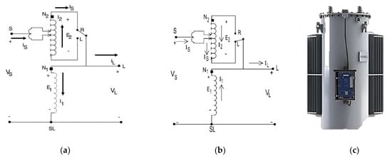
Figure 3. Circuit diagram of a step VR: (a) raise position, (b) lower position, and (c) type B regulator.

The voltage and current equations of the regulator in the raise position, Figure 3a, are expressed as follows:

$$\frac{E_1}{N_1}=\frac{E_2}{N_2}$$

(1)

$$V_S=E_1-E_2$$

(2)

$$V_L=E_1$$

(3)

$$E_2=\left(\frac{N_2}{N_1}\right)E_1=\left(\frac{N_2}{N_1}\right)V_L$$

(4)

$$V_S=\left(1-\frac{N_2}{N_1}\right) V_L$$

(5)

$$V_S=a_R· V_L$$

(6)

$$a_R=\left(1-\frac{N_2}{N_1}\right)$$

(7)

The voltage equations of the regulator in the lower position, Figure 3b, are expressed as follows:

$$V_S=E_1+E_2$$

(8)

$$E_2=\left(\frac{N_2}{N_1}\right),E_1=\left(\frac{N_2}{N_1}\right)V_L$$

(9)

$$V_S=\left(1+\frac{N_2}{N_1}\right)\times V_L$$

(10)

$$V_S=a_R· V_L, a_R=\left(1+\frac{N_2}{N_1}\right)$$

(11)

where V_S denotes the main source voltage, V_L denotes the voltage of the load, and a_R refers to the turns ratio of the VR, defined as a function of the turns ratio of the transformer. E₁ and E₂ are the voltage applied on N₁ and N₂, respectively. A reverse switch must be equipped to control the VR voltage in the range of ±10% of the specified voltage, often in 8, 16, or 32 steps. The 32-step is most commonly employed in substations (16 steps in both voltage increase and voltage decrease positions). Each step corresponds to a voltage change of 0.00625 p.u. (i.e., 0.1/16 p.u). VRs may connect in wye, delta, or open delta for a three-phase system. Bandwidth (BW) should be set to ensure that the taps are changed only when the voltage is out of the BW, and this is specified by a minimum and maximum regulation voltage (set to ±1% of the nominal voltage).

The turns ratio of the voltage regulator can be considered a function of the tap position (TP), as indicated in (12):

$$a_R=\{\begin{array}{c}1-\left(0.00625 · TP\right), raise position\\ 1+\left(0.00625 · TP\right), lower position\end{array}$$

(12)

The reader may refer to [40] for further information on VRs and control circuits.

3.2. Direct Load Flow Approach, including VR Units

An improved direct approach load flow method for radial distribution systems, including VRs, is explored in this section. The proposed technique’s fundamental goal is to obtain the power flow solution and VR optimum tapping positions as quickly as possible. The standard backward/forward sweep approach may be used and offers an accurate solution, but the additional implementation time is the biggest obstacle, since it depends on iterative solutions. The suggested methodology can be considered a combination of optimization and load flow strategies, as it determines the best tapping position and calculates the load flow without repetitive solutions.

The following example illustrates the mathematical formulation of the suggested model: consider the radial system indicated in Figure 4, which consists of seven buses, six branches, and one VR connected directly before bus 4. The branch current can be expressed in terms of the load current by applying the Kirchhoff current law (KCL), as follows:

$$\begin{gathered} I{b}_1=I_2+I_3+\raisebox{1ex}{$I_4$}\!\left/ \!\raisebox{-1ex}{$a_R $}\right.+\raisebox{1ex}{$I_5$}\!\left/ \!\raisebox{-1ex}{$a_R $}\right.+\raisebox{1ex}{$I_6$}\!\left/ \!\raisebox{-1ex}{$a_R $}\right.+I_7 \\ I{b}_2=0+I_3+\raisebox{1ex}{$I_4$}\!\left/ \!\raisebox{-1ex}{$a_R $}\right.+\raisebox{1ex}{$I_5$}\!\left/ \!\raisebox{-1ex}{$a_R $}\right.+\raisebox{1ex}{$I_6$}\!\left/ \!\raisebox{-1ex}{$a_R $}\right.+0 \\ I{b}_3=0+0+\raisebox{1ex}{$I_4$}\!\left/ \!\raisebox{-1ex}{$a_R $}\right.+\raisebox{1ex}{$I_5$}\!\left/ \!\raisebox{-1ex}{$a_R $}\right.+\raisebox{1ex}{$I_6$}\!\left/ \!\raisebox{-1ex}{$a_R $}\right.+0 \\ I{b}_4=0+0+0+I_5+0+0 \\ I{b}_5=0+0+0+0+I_6+0 \\ I{b}_6=0+0+0+0+0+I_7 \end{gathered}$$

(13)

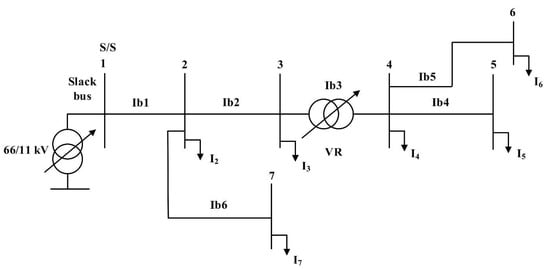
Figure 4. An illustrative example of the direct load flow approach, including VR units.

Equation (13) can be written in the matrix form below.

$$\left[\begin{array}{c}I{b}_1\\ I{b}_2\\ I{b}_3\\ I{b}_4\\ I{b}_5\\ I{b}_6\end{array}\right]=\left[\begin{array}{cccccc}1& 1& 1/a_R& 1/a_R& 1/a_R& 1\\ 0& 1& 1/a_R& 1/a_R& 1/a_R& 0\\ 0& 0& 1/a_R& 1/a_R& 1/a_R& 0\\ 0& 0& 0& 1& 0& 0\\ 0& 0& 0& 0& 1& 0\\ 0& 0& 0& 0& 0& 1\end{array}\right]\left[\begin{array}{c}{I}_2\\ I_3\\ I_4\\ I_5\\ I_6\\ I_7\end{array}\right]$$

(14)

To generalize, Equation (14) can be written in the following form:

$${\left[Ib\right]}_{nl\times 1}={\left[BIB{C}_N\right]}_{nl\times \left(nb-1\right)}\times {\left[I\right]}_{\left(nb-1\right)\times 1}$$

(15)

where nl denotes the number of branches in the system, nb denotes the total number of buses, and $BIB{C}_N$ is the modified bus-injection-to-branch-current matrix.

The bus voltage values of the system can be expressed as a function of branch currents, while the voltage drop across the VR can be neglected; thus,

$$\begin{gathered} v_2=v_1-Z_{12} I{b}_1 \\ {v}_3=v_2-Z_{23} I{b}_2=v_1-Z_{12} I{b}_1-Z_{23} I{b}_2 \\ {v}_4=\left(v_{3 }-Z_{34} I{b}_3\right)/a_R=\left(v_{1 }-Z_{12} I{b}_1-Z_{23} I{b}_2-Z_{34} I{b}_3 \right)/a_R \\ {v}_5=v_4-Z_{45} I{b}_4=\left(v_{1 }-Z_{12} I{b}_1-Z_{23} I{b}_2-Z_{34} I{b}_3 \right)/a_R-Z_{45} I{b}_4 \\ {v}_6=v_4-Z_{46} I{b}_{5 }=\left(v_{1 }-Z_{12} I{b}_1-Z_{23} I{b}_2-Z_{34} I{b}_3 \right)/a_R-Z_{46} I{b}_5 \\ {v}_7=v_2-Z_{27} I{b}_6= v_1-Z_{12} I{b}_1-Z_{27} I{b}_6 \end{gathered}$$

(16)

Equation (16) can be expressed in the following form (matrix form):

$$\left[\begin{array}{c}{V}_2\\ V_3\\ V_4\\ V_5\\ V_6\\ V_7\end{array}\right]=\left[\begin{array}{c}{V}_1\\ V_1\\ V_1/a_R\\ V_1/a_R\\ V_1/a_R\\ V_1\end{array}\right]-\left[\begin{array}{cccccc}{Z}_{12}& 0& 0& 0& 0& 0\\ Z_{12}& Z_{23}& 0& 0& 0& 0\\ Z_{12}/a_{\mathrm{R}}& Z_{23}/a_{\mathrm{R}}& Z_{34}/a_{\mathrm{R}}& 0& 0& 0\\ Z_{12}/a_{\mathrm{R}}& Z_{23}/a_{\mathrm{R}}& Z_{34}/a_{\mathrm{R}}& Z_{45}& 0& 0\\ Z_{12}/a_{\mathrm{R}}& Z_{23}/a_{\mathrm{R}}& Z_{34}/a_{\mathrm{R}}& 0& Z_{46}& 0\\ Z_{12}& 0& 0& 0& 0& Z_7\end{array}\right]\left[\begin{array}{c}I{b}_1\\ I{b}_2\\ I{b}_3\\ I{b}_4\\ I{b}_5\\ I{b}_6\end{array}\right]$$

(17)

To generalize, Equation (17) can be written in the following form:

$${\left[Vb\right]}_{\left(nb-1\right)\times 1}={\left[V_{slac{k}_N}\right]}_{\left(nb-1\right)\times 1}-{\left[BCB{V}_N\right]}_{\left(nb-1\right)\times nl}\times {\left[Ib\right]}_{nl\times 1}$$

(18)

where Vb is the distribution system bus voltage, $V_{slac{k}_N}$ is the modified slack bus voltage considering the VR turns ratio, $BCB{V}_N$ denotes the modified branch-current-to-bus-voltage matrix, and Ib is the branch current.

This load flow method relies on two metrics, BIBC and BCBV. BIBC is the bus-injection-to-branch-current matrix. BIBC matrix rows are associated with the branches of the RDS, while its columns are associated with the bus-injected currents, except for the slack bus. BCBV is the branch-current-to-bus-voltage matrix. Rows of the BCBV matrix are related to the bus-injected currents, except for the slack bus, while its columns are related to the distribution system branches. Further information about the construction of these matrices can be found in [41].

The steps of determining the optimal tapping position of each VR unit can be summarized as follows:

• Insert line data, load data, VR connection point, minimum and maximum regulation voltage, and the pre-defined tap voltage regulator.
• Construct BIBC and BCBV matrices.
• Perform an initial load flow without VRs.
• For the first VR, identify its bus and compare its voltage value with the minimum and maximum regulation voltage. If the voltage exceeds the maximum regulation, update the tapping position and calculate a_R using (19). If the voltage is lower than the minimum regulation voltage, update the tapping position and calculate a_R using (20), where Tapvalue is the tapping value, V(VR_bus) is the voltage of the VR bus, $V_{reg}^{max}$ is the maximum regulation voltage, $V_{reg}^{min}$ is the minimum regulation voltage, $Ta{p}_{pos}^{new}$ denotes the new tapping position, and $Ta{p}_{pos}^{old}$ denotes the old tapping position.

  $$\begin{gathered} Tapvalue=\frac{V\left(V{R}_{bus}\right)- V_{reg}^{max}}{0.00625}, \\ Ta{p}_{pos}^{new}=Ta{p}_{pos}^{old}-Tapvalue, \\ {a}_R=1+\left(0.00625\times Ta{p}_{pos}^{new}\right). \end{gathered}$$

  (19)

  $$\begin{gathered} Tapvalue=\frac{ V_{reg}^{min}– V\left(V{R}_{bus}\right)}{0.00625}, \\ Ta{p}_{pos}^{new}=Ta{p}_{pos}^{old}-Tapvalue, \\ {a}_R=1-\left(0.00625\times Ta{p}_{pos}^{new}\right). \end{gathered}$$

  (20)
• Calculate the BIBC_N and BCBV_N after considering the VRs.
• Perform the load flow with the new matrices and calculate the tapping position.
• Stop and terminate the program if the tapping position is the same in two successive iterations.
• Repeat steps from 3 to 5 if the tapping position is not the same. Stop when the tapping position becomes the same.
• Repeat the above steps for the other VR units.

4. System Studied and Problem Formulation

4.1. System Studied

Figure 5 shows the one-line diagram for the studied Egyptian Talla system (ETS), located in a rural area in Menoufia Governorate, Egypt. It includes 37 buses with a reactive power of 2.9759 MVAr and active power of 4.8019 MW. The reader may refer to [42,43] for further information about ETS, and the system data is given in Appendix A. We aim to present a cost-benefit analysis that contains the fixed and operating costs of the investigated compensators (DGs, CBs, and VRs) and the profits obtained by reducing the active power loss and power bought from the grid when maximizing the allowable HC level of the system.

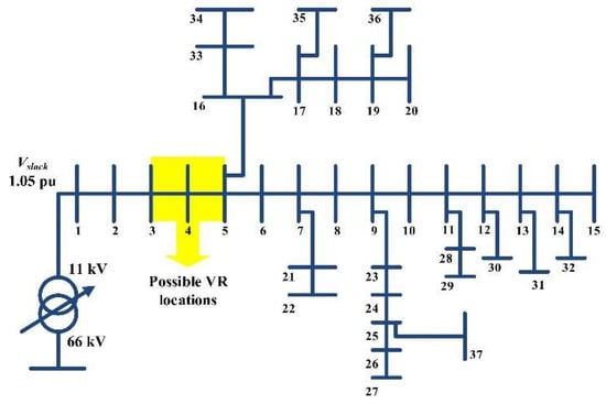
Figure 5. The system under study.

Moreover, we assumed the daily load curve of ETS based on the electricity consumption pattern in this area, as shown in Table 2. This assumption relies on an accurate study of the geographical nature of this rural area and SCADA system measurements. Moreover, five loading levels (LL) are assumed in this study, and each loading level is characterized by a certain percentage of the peak load.

Table 2. Assumed daily load curve of ETS.

Loading Level (LL)	Hour		Percentage of Peak Load (%)
	From	To	From	To
1	1	6	40	60
2	7	12	60	80
3	13	18	80	90
4	19	22	90	100
5	23	24	50	70

Uncertain loading conditions were taken into account in this study. The main load demand clusters were obtained using the soft fuzzy C-means (FCM) clustering approach according to load consumption patterns in this rural area. Each cluster is associated with a unique scenario (centroid) obtained using the FCM algorithm.

Primarily, Dunn developed the FCM clustering technique in 1973 [44], and Bezdek enhanced it in 1981. It is used to divide a collection of data (N) into a predetermined number of clusters (C), where C ≥ 2. The clustered data is collected in a matrix Y, which includes a series of column vectors y_j, where j ∈ {1, 2… N}. FCM needs two parameters for group Y: C and the fuzziness component (m), where m ∈ R and m > 1. The optimization process is supposed to be terminated at a pre-specified tolerance. The FCM algorithm is summarized as follows:

• Step 1: A membership matrix $\left(k={\left[K_{ij}\right]}_{C\times N}\right)$ is randomly initialized, with the sum of each column j in K equaling one. From the available data, random C centroids are initially picked and collected in a vector called c, where $\left(c={\left[c_i\right]}_{1\times c}\right)$.
• Step 2: Using the following function, calculate the new centroids:
  $$c_i=\frac{{\sum }_{i=1}^N{k}_{ij}^m\times y_i}{{\sum }_{i=1}^N{k}_{ij}^m }$$

  (21)
• Step 3: Calculate the membership matrix elements $\left(k={\left[K_{ij}\right]}_{C\times N}\right)$ for each element in Y; thus,
  $$k_{ij}=\frac{1}{{(\frac{y_j-c_i}{y_j-c_p})}^{\frac{2}{m-1}}}$$

  (22)
• Step 4: Determine $F_{FCM}^{\left(t\right)}=\sum _{j=1}^N\sum _{i=1}^c{k}_{ij}^m{y}_j-c_i$, where $F_{FCM}^{\left(t\right)}$ denotes the value of the objective function at the tth iteration.
• Step 5: If $F_{FCM}^{\left(t\right)}$ − $F_{FCM}^{\left(t-1\right)}$ < tolerance, break the optimization process; otherwise, restart the process from Step 2. Further information about the FCM clustering technique can be retrieved from [44,45]. In this work, we obtained the most indicative five scenarios of each loading level at each hour; thus, the whole number of scenarios in this study is set to 120.

4.2. Objective Function

In this article, we consider maximizing the total active power injected from the connected DG units (P_dg) as the primary objective function, which refers to maximizing the allowable HC level when divided by the apparent power of the total connected loads ($S_{load}^{rated}$). The HC is expressed as given in (23).

$$HC (\%)=\frac{P_{dg}}{S_{load}^{rated}}\times 100$$

(23)

The objective function is exposed to several constraints (linear and nonlinear).

4.3. Constraints

In the optimization problem, seven limitations are considered: the max suffix indicates the maximum parameter value, the min suffix indicates the minimum parameter value, and the designer specifies these maximum and minimum values.

4.3.1. Bus Voltage Constraint

The bus voltage magnitude should be kept within the minimum and maximum predetermined levels, as expressed in (24).

$$V^{min}\le V_{i,h,L}\le V^{max},\forall i\in nb,h\in H, L\in N_l$$

(24)

where V^min and V^max represent the defined minimum and maximum bus voltage magnitude, respectively, where the minimum and maximum values are considered to be 0.9 and 1.1 p.u., respectively. H is the total number of hours considered in this study (i.e., 24 h). N_l denotes the number of the LLs given in Table 1 (i.e., N_l = 5).

4.3.2. Line Capacity Constraint

The branch currents are limited by their thermal limits, as expressed in (25).

$$I_{br,h,L }\le I_{br}^{max}, \forall br\in nl,h\in H, L\in N_l$$

(25)

where $I_{br}^{max}$ represents the maximum current carrying capacity of the branch.

4.3.3. DG Capacity Constraint

The size of the DG should not be greater than the maximum size limit or the penetration level, as expressed in (26), to avoid the voltage rise or any other concerns related to the power quality in the distribution system.

$$0\le P_{dg}\left(g\right)\le P_{dg}{\left(g\right)}^{max} , \forall g\in N_{dg}$$

(26)

where N_dg represents the total number of DGs, P_dg denotes the size of the DG unit, and g is the DG number.

4.3.4. CB Capacity Constraint

The CBs’ size should not exceed the defined maximum size limit, as formulated in (27).

$$0\le Q_c\left(q\right)\le Q_c{\left(q\right)}^{max}, \forall q\in N_C$$

(27)

where N_c represents the number of CBs, and Q_c denotes the size of CB.

4.3.5. Power Factor Constraint

The power factor (PF) must be specified within certain minimum and maximum values to ensure optimal energy transfer; thus, the PF is limited as expressed in (28).

$$P{F}^{min} \le PF \le P{F}^{max}$$

(28)

where PF^min and PF^max denote the distribution system’s minimum and maximum allowable PF. The minimum and maximum values are assumed to be within 0.92 lagging and unity, respectively.

4.3.6. Power Balance Equality Constraints

The power system constraints are expressed in (29) and (30), and they should be met at each loading level.

$$P_g+{{\displaystyle \sum }}_{g=1}^{N_{dg}}{P}_{dg} \left(g\right)={{\displaystyle \sum }}_{br=1}^{nl}{P}_{loss}\left(br\right)+{{\displaystyle \sum }}_{i=1}^{nb}{P}_d \left(i\right)$$

(29)

$$Q_g+{{\displaystyle \sum }}_{q=1}^{N_C}{Q}_c\left(q\right)={{\displaystyle \sum }}_{br=1}^{nl}{Q}_{loss}\left(br\right)+{{\displaystyle \sum }}_{i=1}^{nb}{Q}_d \left(i\right)$$

(30)

where P_g and Q_g are the real and reactive power of the utility, respectively; P_loss and Q_loss denote the real and imaginary power losses; and P_d and Q_d represent the active and reactive power of the loads.

4.3.7. Reverse Power Flow Constraint

The two cases suggested to maximize HC in this work are given as follows:

• Case 1: It is assumed that the distribution network operator (DNO) has upgraded facilities to deal with the system’s bi-directional power flow (that may occur due to the DGs), and thus reverse power flow might be allowed in the system’s branches;
• Case 2: The DNO restricts the reverse power flow in the system’s branches.
  $$\tau \times P_{Line}^{br} \ge 0, \forall br\in nl, \tau =\left\{0,1\right\}$$

  (31)

  where $P_{Line}$ denotes the net active power flow in each branch. Algorithmically, Case 1 is activated when the decision variable τ is set to 0, while Case 2 is activated when the decision variable τ is set to 1.

4.4. Constraints Handling

The penalty methods are widely used for handling optimization constraints. Several penalty methods are used in the literature, such as static, dynamic, death, and others. In this work, we used a static penalty method (large number), in which a constant penalty coefficient is multiplied by the constraint and merged with the objective function. Accordingly, the best fitness function corresponds to the best-unpenalized value of the objective function when all the constraints are satisfied [46].

4.5. System Performance Assessment

This section presents different technical and economic indices that describe the system under investigation’s performance.

4.5.1. Technical PQ Performance Indices

• Benefits due to reduction of the real power loss (B₁)

The real power loss of the system after compensation should be lower than the system power loss before compensation. The annual benefit gained (USD/year) from such a reduction is expressed in (32), where w₁ denotes the active power rate (USD/kWh), and its numerical value is set to USD 0.06/kWh [43].

$$B_1=365\times w_1\times {\displaystyle \sum }_{h=1}^{h=24}\left[ \left(P_{loss,h}^{before}-P_{loss,h}^{after}\right)\right]$$

(32)

• Benefits due to reduction of the purchased complex power (B₂)

The annual reduction of the apparent power (USD/year) purchased from the utility is expressed in (33), where w₂ denotes the tariff rate of the apparent power (USD/kVAh) and is assumed to be USD 0.06/kVAh [43].

$$B_2=365\times w_2\times {\displaystyle \sum }_{h=1}^{h=24}\left[ \left(S_{grid,h}^{before}-S_{grid,h}^{after}\right)\right]$$

(33)

• Loading capacity enhancement (B₃)

The loading capacity (LC) is formulated by dividing each branch’s current value by the current carrying capacity of this branch at the worst scenario obtained in LL₄ (which represents the peak loading level at hours 19, 20, 21, and 22), as formulated in (34).

$$B_3=\mathit{max}\left(LC\right)=\mathit{max}\left(\frac{I_{br,h}}{I_{br}^{max}}\right),\forall br\in nl, h=\left\{19,20,21,22\right\}$$

(34)

• Voltage stability enhancement (B₄)

The voltage stability index (VSI) enhancement is formulated by determining the VSI calculated at all buses, picking the minimum one, as given in Equation (35), and comparing its value with the value obtained in the uncompensated case at the worst scenario obtained in LL₄.

$$B_4=\mathit{min}\left[VS{I}_{bus}\right]=V_i^4-4{\left(PX-QR\right)}^2-4V_i^2\left(PR+QX\right),\forall i\in nb, h=\left\{19,20,21,22\right\}$$

(35)

where V_i denotes the bus i sending-end voltage, R refers to the transmission line resistance, X denotes the line reactance, P refers to the transferred real power within the line, and Q represents the transferred reactive power throughout the line.

4.5.2. Economic Evaluation

• Costs of DGs (C_DG)

C_DG denotes the investment costs of the DGs (costs to be paid in USD/year) as formulated in (36), where OM_DG represents DGs’ operation and maintenance costs. RF_DG describes the capital recovery factor of DGs, which converts the present value cost to an annualized cost. OM_DG is set to USD 5/W.

$$C_{DG}=O{M}_{DG}\times R{F}_{DG}\times {\displaystyle \sum }_{g=1}^{N_{dg}}{P}_{dg}\left(g\right)$$

(36)

• Costs of CBs (C_CBs)

C_CBs denotes investment costs of the CBs, as expressed in (37), where O_CB represents CBs’ operation costs, FC_CB means CBs’ fixed installation costs, and RF_CB denotes CBs’ capital recovery factor. O_CB and FC_CB are set to USD 30/kVAr and USD 1000, respectively.

$$C_{CB}=R{F}_{CB}\left[F{C}_{CB}+{\displaystyle \sum }_{q=1}^{N_C }{O}_{CB}\times Q_C\left(q\right)\right]$$

(37)

• Costs of VRs (C_VR)

C_VR (USD/year) is expressed in Equation (38), where RF_VR represents the capital recovery factor of VRs. R₀ is the VR’s cost (USD), which relies on the current rating of the VR (I_VR). For instance, R₀ equals USD 38,000 for 100 A, USD 44,800 for 150 A, USD 50,600 for 200 A, USD 58,100 for 250 A, USD 64,700 for 300 A, USD 70,300 for 350 A, and USD 77,900 for 400 A [43].

$$C_{VR}=R{F}_{VR}\times R_0\left(I_{VR}\right)$$

(38)

A generalized formula of the different compensators’ capital recovery factors (RF_k) is expressed in Equation (39), where int is the annual interest rate, and it is assumed to be 7%, while LT denotes the lifetime of the connected compensator. In this study, the lifetime of the components is taken as twenty years for the DGs, ten years for the CBs, and fifteen years for the VRs.

$$R{F}_k=\frac{int\times {\left(1+int\right)}^{LT}}{{\left(1+int\right)}^{LT}-1},\forall k=\left\{DG,CB,VR\right\}$$

(39)

• Total savings (TS)

Finally, the total saving after allocating the compensators is defined as the difference between the total benefits and costs, as expressed in (40).

$$TS=\left[B_1+B_2\right]-\left[C_{DG}+C_{CB}+C_{VR}\right]$$

(40)

Finally, Figure 6 shows the hierarchical formulation of the problem studied.

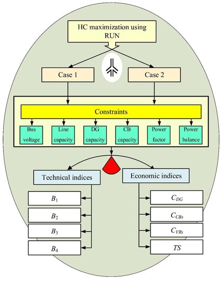
Figure 6. Hierarchical formulation of the problem studied.

4.6. RUN Optimization Technique

Nowadays, optimization algorithms are usually needed to solve complex engineering problems in different applications [47,48,49,50,51]. In this study, RUN is applied to solve the proposed problem. RUN was developed in 2021 by Ahmadianfar et al. [52]. Its idea relies on the Runge–Kutta (RK) theory to find the numerical solution for ordinary differential equations. Like any other optimization technique, the RUN consists of three phases: (a) the initialization process, (b) the updating phase, and (c) the evaluation phase. The mechanism of the RUN is depicted in Figure 7. The RUN has been employed in many applications, such as (a) reconfiguring the partially shaded PV array to maximize its generated power [53], (b) enhancing the reliability of the power system and increasing renewables penetration [54], and (c) finding the optimal tuning of different power system stabilizer controllers [55].

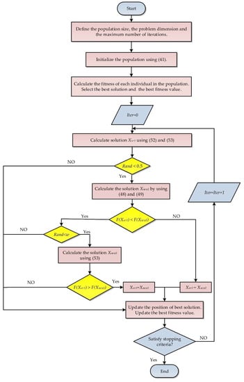
Figure 7. Mechanism of operation of the RUN algorithm.

4.6.1. Initialization

A population of size N and dimension D is randomly generated using (41). U_l and L_l refer to the upper and lower bounds of the lth variable, and rand is a uniformly distributed random value in the range [0, 1].

$$x_{n,l}=L_l+rand\times \left(U_l-L_l\right)$$

(41)

4.6.2. Updating and Evaluation Phases

In the RUN algorithm, the decision variables are subjected to three steps of updating. The first stage uses a search mechanism (SM) based on the RK method for updating the position of each individual in the population, as explained in (42) and (43). If the random value rand is less than 0.5, the new positions are determined by (42). Otherwise, they are calculated by (43). More details about SM can be found in [52].

$$x_{n+1}=\left(x_c+r\times SF\times g\times x_c\right)+SF\times SM+\mu \times randn\times (x_m-x_c)$$

(42)

$$x_{n+1}=\left(x_m+r\times SF\times g\times x_m\right)+SF\times SM+\mu \times randn\times \left(x_{r1}-x_{r2}\right)$$

(43)

where r is an integer that equals 1 or −1, $g$ is a random value in the range [0, 2], and $\mu$ is a random number with normal distribution; $SF$ is an adaptive factor calculated by (44) and (45); and $x_c$ and $x_m$ are obtained by (46) and (47), respectively.

$$SF=2\left(0.5-rand\right)\times f$$

(44)

$$f=a\times exp\left(-b\times rand\times \left(\frac{i}{Maxi}\right)\right)$$

(45)

$$x_c=\phi \times x_n+\left(1-\phi \right)\times x_{r1}$$

(46)

$$x_m=\phi \times x_{best}+\left(1-\phi \right)\times x_{lbest}$$

(47)

where $Maxi$ refers to the maximum number of iterations, a and b are constant numbers, i denotes the number of the current iteration, $\phi$ is a random value in the range of (0, 1), $x_{best}$ represents the best solution obtained so far, and $x_{lbest}$ denotes the best position found at each iteration.

In the second stage, the enhanced solution quality scheme, formulated in (48) and (49), is executed to improve the quality of the solutions obtained. The new variable x_new2 is obtained by (48) if w < 1; otherwise, x_new2 is computed by (49). It is worth mentioning that Equations (48) and (49) are carried out if a randomly generated value between 0 and 1 is less than 0.5.

$$x_{new2}=x_{new1}+r\times w\times |\left(x_{new1}-x_{avg}\right)+randn|$$

(48)

$$x_{new2}=\left(x_{new1}-x_{avg}\right)+r\times w\times |\left(u\times x_{new1}-x_{avg}\right)+randn|$$

(49)

where β is a random value in the range of [0, 1]; c is a random value equal to 5 × rand; x_best denotes the best solution obtained so far; and w, x_avg, and x_new1 are calculated using (50)–(52), respectively.

$$w=rand\left(0, 2\right)\times exp\left(-c\left(\frac{i}{Maxi}\right)\right)$$

(50)

$$x_{avg}=\frac{x_{r1}+x_{r2}+x_{r3}}{3}$$

(51)

$$x_{new1}=\beta \times x_{avg}+\left(1-\beta \right)\times x_{best}$$

(52)

If the fitness value of $x_{new2}$ is greater than the fitness of $x_{n+1}$, the third stage is conducted, and the new position $x_{new3}$ is generated as expressed in (53). The third stage provides another chance to boost the solution quality of the RUN algorithm.

$$x_{new3}=\left(x_{new2}-rand\times x_{new2}\right)+SF(rand\times x_{RK}+\left(v\times x_b-x_{new2}\right))$$

(53)

where $v$ is a random number with a value of $2\times rand$.

5. Numerical Results and Discussion

5.1. Uncompensated System

The decision variables of the investigated problem under study are the location and sizes of DGs and CBs and the tapping positions of the VRs. The locations are considered integer variables and are set to be from 2 to N_buses (system number of buses). The discrete CB sizes are assumed to be from 0 to 1200 kVAr in a 150 kVAr step. It should be noted that more than one capacitor can be connected to the same bus. The DG sizes are assumed to be continuous in the 0–2 MW range. The numbers of CBs and DGs are considered to be seven and three, respectively, plus one VR location. These mixed variables—locations and sizes—are produced randomly within their allowable ranges. Then, the RUN optimization algorithm is used for solving this issue and calculating the optimal values for these parameters when HC maximization is considered. The backward/forward sweep algorithm performs the load flow. Table 3 explores the values of the load demand in percentages and the probability of occurrence of the corresponding demand scenarios for the system under investigation given in Figure 5.

Table 3. Values of the load demand and probability of occurrence of the corresponding demand scenarios.

Hour	Load Percentage (%)					Probability (p)
	C1	C2	C3	C4	C5	p1	p2	p3	p4	p5
1	41.997	45.699	49.780	54.001	58.149	0.212	0.176	0.216	0.231	0.165
2	41.797	46.296	50.756	54.461	58.315	0.188	0.241	0.205	0.185	0.181
3	41.685	45.801	50.151	54.149	58.136	0.192	0.197	0.217	0.210	0.184
4	41.742	46.008	50.401	54.501	58.391	0.210	0.202	0.197	0.190	0.201
5	41.842	45.630	49.705	53.584	57.811	0.186	0.205	0.194	0.205	0.210
6	41.811	45.998	50.257	54.428	58.382	0.178	0.200	0.206	0.217	0.199
7	61.897	66.200	70.181	74.241	78.337	0.193	0.204	0.209	0.214	0.180
8	61.870	65.681	69.769	73.926	78.161	0.169	0.198	0.222	0.204	0.207
9	61.757	65.696	69.632	73.850	78.222	0.180	0.184	0.191	0.225	0.220
10	61.844	66.234	70.371	74.640	78.138	0.220	0.197	0.179	0.206	0.198
11	62.031	66.262	70.440	74.322	78.189	0.196	0.210	0.220	0.198	0.176
12	61.629	65.638	69.906	73.891	78.052	0.178	0.215	0.227	0.207	0.173
13	81.005	83.262	85.381	87.367	89.208	0.203	0.237	0.177	0.210	0.173
14	81.049	83.200	85.349	87.373	89.248	0.193	0.214	0.225	0.198	0.170
15	80.957	83.193	85.104	87.033	89.009	0.200	0.199	0.182	0.207	0.212
16	81.219	83.395	85.500	87.485	89.317	0.226	0.224	0.214	0.170	0.166
17	80.915	82.825	84.846	87.080	89.155	0.182	0.189	0.204	0.240	0.185
18	80.713	82.664	84.950	87.010	89.145	0.187	0.200	0.227	0.182	0.204
19	90.929	92.990	95.048	97.070	99.058	0.165	0.226	0.204	0.208	0.197
20	90.820	92.920	94.921	97.120	99.230	0.185	0.197	0.229	0.190	0.199
21	90.994	93.015	95.279	97.459	99.203	0.214	0.213	0.209	0.213	0.151
22	90.785	92.787	94.912	97.070	99.192	0.201	0.196	0.209	0.210	0.184
23	51.652	55.493	59.533	63.825	68.106	0.193	0.199	0.195	0.223	0.190
24	51.711	55.461	59.519	63.770	67.997	0.188	0.166	0.232	0.216	0.198

Table 4 presents the results of ETS’s initial load flow without applying any enhancement technique (base case). It can be noted that the system’s losses (active and reactive) are very high, especially in high loading conditions (i.e., LL₃ and LL₄). Figure 8 shows the active power loss, reactive power loss, and complex power purchased from the grid throughout the day. It can be seen that the active power loss, reactive power loss, and complex purchased power from the utility are significantly high, especially at hours 19–22, due to the high loading conditions.

Table 4. Results obtained for the uncompensated base ETS.

Parameter	Value
Ploss (MW)	14.81
Qloss (MVAr)	20.02
Sgrid (MVA)	121.28
LC at h = 19	0.7320
LC at h = 20	0.7554
LC at h = 21	0.7879
LC at h = 22	0.8105
VSImin at h = 19	0.3545
VSImin at h = 20	0.3382
VSImin at h = 21	0.3167
VSImin at h = 22	0.3020

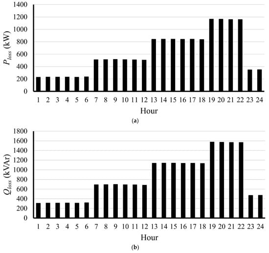
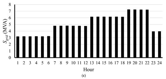
Figure 8. Results obtained for the uncompensated base ETS throughout the day: (a) active power loss, (b) reactive power loss, and (c) apparent power purchased from the grid.

Figure 9a illustrates the minimum values of the bus voltage magnitudes of the uncompensated ETS at hours 4 and 20, respectively, in which hour 4 represents the light loading condition, and hour 20 represents the peak loading condition. In addition, Figure 9b shows the maximum bus voltage magnitudes at the same chosen hours. Minimum and maximum bus voltage magnitudes were obtained by obtaining minimum and maximum values for the five scenarios per hour. The bus voltage magnitudes can be considered slightly low due to the geographical nature of the system, where the system contains some long branches (about 13 km for branches 3–4 and 4–5). These are the possible locations for the VR, as marked in Figure 5. Moreover, the branch currents at hour 20 are slightly high due to the peak loading conditions. Figure 10 shows the base case system’s current values (minimum and maximum values of each branch current) at the same chosen hours.

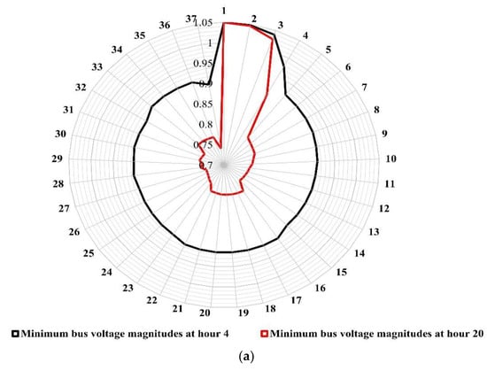
Figure 9. Values of the bus voltage magnitudes of the uncompensated ETS at hours 4 and 20: (a) minimum and (b) maximum.

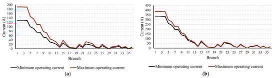
Figure 10. Values of the branch current magnitudes of the uncompensated ETS at: (a) hour 4 and (b) hour 20.

5.2. Compensated System

The RUN optimization algorithm has been used to obtain the optimal allocation of the compensators used for the performance enhancement of ETS. In the two cases considered, we assumed that the candidate locations for one VR are (i) between buses 4–5 or (ii) between buses 3–4.

• Results obtained in Case 1

In this case, it was assumed that the DNO has upgraded facilities to deal with the system’s bi-directional power flow, which may occur due to the DGs, and thus reverse power flow might be allowed in the system’s branches. The output results are shown in Table 5, considering that the candidate location of the VR is before bus 5, while Table 6 shows the detailed results if the candidate location for the VR is before bus 4.

Table 5. Results obtained for the compensated ETS with one VR between buses 4 and 5 while allowing reverse power to flow: Case 1.

Parameter	Value	Parameter	Value
Ploss (MW)	1.60	TP at h = 23, 24	−12
Qloss (MVAr)	1.71	Cost of CBs (USD/year)	19,363.34
Sgrid (MVA)	70.72	Cost of DGs (USD/year)	1,359,796.16
Optimal CBs locations	2, 6, 7	Cost of VRs (USD/year)	4918.80
Optimal CBs sizes (kVAr)	2850, 450, 1200	Benefits (USD/year)	1,396,747.20
Optimal DGs locations	12, 2, 7	Total saving (USD/year)	12,668.90
Optimal DGS sizes (kW)	1818.499, 1999.999, 983.402	HC (%)	100.00
TP at h = 1, 2, 3, 4, 5, 6	−15	LC at h = 19	0.2963
TP at h = 7, 8, 10, 11	−8	LC at h = 20	0.2971
TP at h = 9, 12	−9	LC at h = 21	0.3000
TP at h = 13, 14, 15, 16, 17, 18	−2	LC at h = 22	0.3044
TP at h = 19, 21	4	VSImin at h = 19, 20	0.9206, 0.9122
TP at h = 20, 22	3	VSImin at h = 21, 22	0.8981, 0.8844

Table 6. Results obtained for the compensated ETS with one VR between buses 3 and 4 while allowing reverse power to flow: Case 1.

Parameter	Values	Parameter	Values
Ploss (MW)	2.35	Cost of DGs (USD/year)	1,359,796.09
Qloss (MVAr)	2.76	Cost of VRs (USD/year)	5555.61
Sgrid (MVA)	98.83	Benefits (USD/year)	764,712.45
Optimal CBs locations	4, 2, 13	Total saving (USD/year)	−625,128.18
Optimal CBs sizes (kVAr)	450, 4350, 900	HC (%)	100.00%
Optimal DGs locations	17, 7, 2	LC at h = 19	0.4140
Optimal DGS sizes (kW)	805.3462, 1999.999, 1996.554	LC at h = 20	0.4265
TP at h = 1, 2, 3, 4, 5, 6	−12	LC at h = 21	0.4391
TP at h = 7, 8, 9, 10, 11, 12	−8	LC at h = 22	0.4506
TP at h = 13, 14, 15, 16, 17, 18	−4	VSImin at h = 19	0.7155
TP at h = 19, 20, 21, 22	−2	VSImin at h = 20	0.6969
TP at h = 23, 24	−10	VSImin at h = 21	0.6952
Cost of CBs (USD/year)	24,889.31	VSImin at h = 22	0.6783

Although the system operating HC reaches 100% in the two candidate locations for the VR, the real power loss, reactive power loss, and complex power purchased from the grid throughout the day in the first location are less than their corresponding values in the second location, so we decided to visualize the results obtained when using the first VR location. Figure 11 illustrates the real power loss, reactive power loss, and complex power purchased from the grid throughout the day. It is apparent that the system losses (i.e., active and reactive) and the purchasing power from this grid in the candidate’s two locations are significantly decreased compared with the base case due to the optimal coordination allocation of DG units, CBs, and VRs.

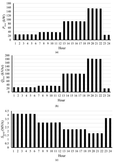
Figure 11. Results obtained for the compensated base ETS throughout the day while allowing reverse power flow: (a) active power loss, (b) reactive power loss, and (c) apparent power purchased from the grid.

Figure 12a presents the minimum values of the bus voltage magnitudes of the compensated ETS at hours 4 and 20, respectively. Moreover, Figure 12b shows the maximum bus voltage magnitudes at the same chosen hours. Figure 13 illustrates the compensated system’s minimum and maximum branch current values at the same investigated hours.

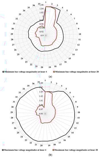
Figure 12. Values of the bus voltage magnitudes of the compensated ETS at hours 4 and 20 while allowing reverse power flow: (a) minimum and (b) maximum.

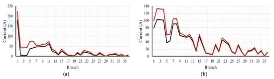
Figure 13. Values of the branch current magnitudes of the compensated ETS while allowing reverse power flow at: (a) hour 4 and (b) hour 20.

Figure 12 and Figure 13 present the bus voltage magnitudes and system branch currents after compensation, in which the current of each branch is decreased, and the bus voltage magnitudes are enhanced within the allowable limits. The minimum voltage at hour 4 is improved to 0.9792 p.u, compared to 0.8996 p.u at the base case; and the maximum voltage at hour 4 is increased to 1.0839 p.u (preserved within the acceptable limits), compared to 1.05 p.u at the base case. Moreover, the minimum voltage at hour 20 is improved to 0.9365 p.u, compared to 0.7411 p.u at the base case. The benefits achieved in this case can be summarized as follows: the active power loss is reduced from 14.81 MW in the base case to 1.60 while VR is in its first location and reaches 2.35 MW in the second location, and the reactive power loss is reduced from 20.02 MVAr in the base case to 1.71 MVAr in the first location and becomes 2.76 MVAr in the second location. Besides, the complex power purchased from the utility is significantly decreased in the first location to 70.72 MVA, and 98.83 MVA in the second location, compared with the 121.28 MVA base case.

In addition, at h = 19, the LC of the system is improved to 0.2963 in the first location and 0.4140 in the second location, compared to 0.7320 in the base case. Moreover, the VSI_min at the same hour is improved to be 0.9206 in the first location and 0.7155 in the second location, compared to 0.3545 in the base case.

In the first possible VR location, the revenue obtained from power loss and total power reduction is USD 1.3967 million annually. The total saving, defined as compensators’ benefits minus their costs, is annually about USD 0.0127 million.

• Results obtained in Case 2

In this case, it was assumed that the DNO restricts the reverse power flow in the system’s branches. The output results are explored in Table 7, considering that the suggested location of the VR is between buses 4 and 5, while Table 8 illustrates the detailed results if the proposed location for the VR is between buses 3 and 4.

Table 7. Results obtained for the compensated ETS with one VR between buses 4 and 5, no reverse power to flow: Case 2.

Parameter	Value	Parameter	Value
Ploss (MW)	12.28	Cost of DGs (USD/year)	886,938.2825
Qloss (MVAr)	14.17	Cost of VRs (USD/year)	7103.7122
Sgrid (MVA)	61.97	Benefits (USD/year)	1,354,359.219
Optimal CBs locations	13, 37, 27, 6, 10, 4, 23	Total saving (USD/year)	442,235.2809
Optimal CBs sizes (kVAr)	150, 1200, 1050, 150, 150, 1200, 300	HC (%)	49%
Optimal DGs locations	2, 3	LC at h = 19	0.6920
Optimal DGs sizes (kW)	2119.368, 229.6908	LC at h = 20	0.6922
TP at h = 1, 2, 3, 4, 5, 6	−14	LC at h = 21	0.6824
TP at h = 7, 8, 10, 11	−6	LC at h = 22	0.6756
TP at h = 9, 12	−7	VSImin at h = 19	0.8651
TP at h = 13, 14, 15, 16, 17, 18	1	VSImin at h = 20	0.8476
TP at h = 19, 20, 21, 22	12	VSImin at h = 21	0.8143
TP at h = 23, 24	−10	VSImin at h = 22	0.7914
Cost of CBs (USD/year)	18,081.9428

Table 8. Results obtained for the compensated ETS with one VR between buses 3 and 4, no reverse power to flow: Case 2.

Parameter	Value	Parameter	Value
Ploss (MW)	11.41	Cost of DGs (USD/year)	881,647.6346
Qloss (MVAr)	12.86	Cost of VRs (USD/year)	7103.7122
Sgrid (MVA)	94.07	Benefits (USD/year)	670,524.0625
Optimal CBs locations	37, 19, 2, 8, 12	Total saving (USD/year)	−243,356.9135
Optimal CBs sizes (kVAr)	1200, 150, 2400, 600, 300	HC (%)	49%
Optimal DGs locations	3, 19	LC at h = 19	0.6175
Optimal DGs sizes (KW)	2224.8278, 110.2191	LC at h = 20	0.6113
TP at h = 1, 2, 3, 4, 5, 6	−12	LC at h = 21	0.6096
TP at h = 7, 8, 9, 10, 11, 12	−8	LC at h = 22	0.6103
TP at h = 13, 14, 15, 16, 17, 18	−3	VSImin at h = 19	0.7390
TP at h = 19, 20, 21, 22	−1	VSImin at h = 20	0.7149
TP at h = 23, 24	−10	VSImin at h = 21	0.7114
Cost of CBs (USD/year)	25,129.6292	VSImin at h = 22	0.5627

Figure 14 shows the real power loss, reactive power loss, and complex power purchased from the grid throughout the day. It can be noted that the system power losses and the power supplied by the utility are higher than their values in the case of allowing reverse power flow, which is accompanied by changing the protection system settings.

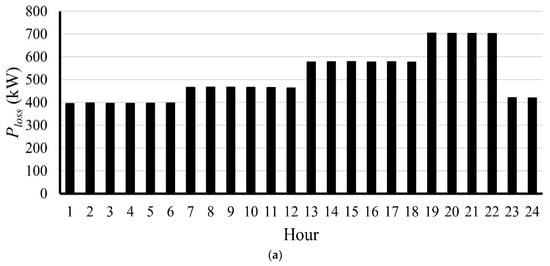
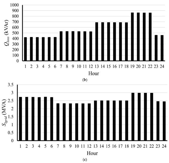
Figure 14. Results obtained for the compensated base ETS throughout the day while not allowing reverse power flow: (a) active power loss, (b) reactive power loss, and (c) apparent power purchased from the grid.

Figure 15a shows the minimum values of the bus voltage magnitudes of the compensated ETS while not permitting reverse power flow at hours 4 and 20, respectively. Moreover, Figure 15b presents the maximum bus voltage magnitudes at the same chosen hours. It can be noted that the minimum voltage magnitude at hour 4 is 0.9823 p.u, compared to 0.8996 p.u at the base case. Moreover, the minimum voltage magnitude at hour 20 is 0.9028 p.u, compared with 0.7411 p.u at the base case.

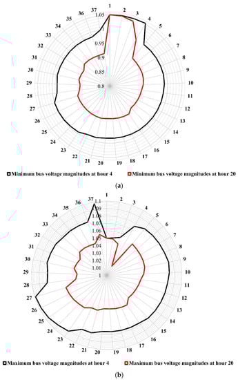
Figure 15. Values of the bus voltage magnitudes of the compensated ETS at hours 4 and 20 while not allowing reverse power flow: (a) minimum and (b) maximum.

Figure 16 shows the compensated system’s minimum and maximum branch current values while not allowing reverse power flow at the same hours. At hour 4, the current value of the first branch drops from 190.26 A in the base case to 158.12 A. In addition, at hour 20, the current value for the same branch drops from 386.04 A in the base case to 159.10 A.

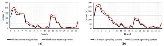
Figure 16. Values of the branch current magnitudes of the compensated ETS while not allowing reverse power flow at: (a) hour 4 and (b) hour 20.

The benefits achieved in this case can be summarized as follows: the active power loss is reduced from 14.81 MW in the base case to 12.28 MW while VR is in its first location and reaches 11.41 MW in the second location, and the reactive power loss is reduced from 20.02 MVAr in the base case to 14.17 MVAr in the first location and becomes 12.86 MVAr in the second location. The complex power purchased from the utility is significantly decreased in the first location to 61.97 MVA, and 94.07 MVA in the second location, compared with the 121.28 MVA base case.

In addition, the LC of the system at h = 19 is improved to 0.6920 in the first location and 0.6175 in the second location compared to 0.7320 in the base case. Moreover, the VSI_min at the same hour is improved to 0.8651 in the first location, and 0.7390 in the second location, compared to 0.3545 in the base case.

The benefits of power loss and apparent power reduction in the first possible VR location are USD 1.3543 million annually. Moreover, the annual total saving is USD 0.4423 million.

Finally, it should be noted that allowing reverse power flow necessities updating the network protection setting and configurations in the presence of renewables and reverse fault currents. Multiple working groups and researchers worldwide are currently working on analyzing and resolving these issues. Conversely, it would be an oversimplification to say that reverse power flow should be avoided. It was apparent in this work that one of the advantages of allowing this reverse power is increasing the HC to reach 100%, while it only reaches 49% when not permitting it.

6. Conclusions and Future Works

This paper proposes the RUN optimization algorithm to solve the optimal coordination problem between DGs, CBs, and VRs in the studied ETS. The results validate that RUN is an efficient optimization tool due to its high convergence speed and balance between exploration and exploitation in solving engineering optimization problems. The soft fuzzy C-means clustering approach considered daily load variations through different loading conditions (i.e., five loading levels). The objective is to maximize the HC under linear and nonlinear constraints in two cases: the first one allows reverse power flow in the system’s branches, and the second one restricts reverse power flow in the system’s branches. The optimal active and reactive power compensators and voltage regulators have been able to maximize the hosting capacity, reduce the system’s total real and reactive power losses, reduce the bought power from the grid, and improve the loading capability and stability of the system.

The optimal allocation of the different units in the distribution system provides a practical technical and economic benefit to the distribution system. The suggested model successfully allocated the different equipment (DGs, CBs, and VRs) for the two studied scenarios. In the case of allowing reverse power flow to the grid while the VR is before bus five, the costs of the compensators are USD 1.384 million per year, and the benefits gained by power loss and total power reduction are USD 1.3967 million per year; therefore, the total saving, defined as the benefits minus the costs, is USD 0.0127 million per year. In the case of restricting the reverse power flow to the grid while VR is in the same location, the equipment costs are USD 0.912 million per year, and the benefits obtained by power loss and complex power reduction are USD 1.3543 million per year; therefore, the total saving is USD 0.4423 million per year. Significant savings occur due to the optimal coordination allocation of DGs, CBs, and VRs at an acceptable voltage profile. This voltage profile improvement is due to the distribution of the capacitors bank at different laterals. We presented HC solutions with and without permission of reverse power flow, allowing or restricting reverse power flow, and the related protection issues are still under investigation in the Egyptian distribution codes. Finally, the integration of energy storage systems will be considered in future works.

References

- Haghighat, H. Energy loss reduction by optimal distributed generation allocation in distribution systems. Int. Trans. Electr. Energy Syst. 2015, 25, 1673–1684. [Google Scholar] [CrossRef]
- Kanwar, N.; Gupta, N.; Niazi, K.R.; Swarnkar, A.; Bansal, R.C. Simultaneous allocation of distributed energy resource using improved particle swarm optimization. Appl. Energy 2017, 185, 1684–1693. [Google Scholar] [CrossRef]
- Ali, Z.M.; Aleem, S.H.E.A.; Omar, A.I.; Mahmoud, B.S. Economical-Environmental-Technical Operation of Power Networks with High Penetration of Renewable Energy Systems Using Multi-Objective Coronavirus Herd Immunity Algorithm. Mathematics 2022, 10, 1201. [Google Scholar] [CrossRef]
- Rawa, M.; Abusorrah, A.; Bassi, H.; Mekhilef, S.; Ali, Z.M.; Abdel Aleem, S.H.E.; Hasanien, H.M.; Omar, A.I. Economical-technical-environmental operation of power networks with wind-solar-hydropower generation using analytic hierarchy process and improved grey wolf algorithm. Ain Shams Eng. J. 2021, 12, 2717–2734. [Google Scholar] [CrossRef]
- Abdelaziz, A.Y.; Hegazy, Y.G.; El-Khattam, W.; Othman, M.M. A multiobjective optimization for sizing and placement of voltage-controlled distributed generation using supervised big bang-big crunch method. Electr. Power Compon. Syst. 2015, 43, 105–117. [Google Scholar] [CrossRef]
- Abdelaziz, A.Y.; Ali, E.S. Static VAR Compensator Damping Controller Design Based on Flower Pollination Algorithm for a Multi-machine Power System. Electr. Power Compon. Syst. 2015, 43, 1268–1277. [Google Scholar] [CrossRef]
- Khodabakhshian, A.; Andishgar, M.H. Simultaneous placement and sizing of DGs and shunt capacitors in distribution systems by using IMDE algorithm. Int. J. Electr. Power Energy Syst. 2016, 82, 599–607. [Google Scholar] [CrossRef]
- Almalaq, A.; Alqunun, K.; Refaat, M.M.; Farah, A.; Benabdallah, F.; Ali, Z.M.; Aleem, S.H.E.A. Towards Increasing Hosting Capacity of Modern Power Systems through Generation and Transmission Expansion Planning. Sustainability 2022, 14, 2998. [Google Scholar] [CrossRef]
- Zobaa, A.F.; Aleem, S.H.E.A.; Abdelaziz, A.Y. Classical and Recent Aspects of Power System Optimization; Academic Press: Cambridge, MA, USA; Elsevier: Amsterdam, The Netherlands, 2018; ISBN 9780128124413. [Google Scholar]
- Rabiee, A.; Mohseni-Bonab, S.M. Maximizing hosting capacity of renewable energy sources in distribution networks: A multiobjective and scenario-based approach. Energy 2017, 120, 417–430. [Google Scholar] [CrossRef]
- Yazdavar, A.H.; Shaaban, M.F.; El-Saadany, E.F.; Salama, M.M.A.; Zeineldin, H.H. Optimal Planning of Distributed Generators and Shunt Capacitors in Isolated Microgrids with Nonlinear Loads. IEEE Trans. Sustain. Energy 2020, 11, 2732–2744. [Google Scholar] [CrossRef]
- Elattar, E.E.; Shaheen, A.M.; El-Sayed, A.M.; El-Sehiemy, R.A.; Ginidi, A.R. Optimal Operation of Automated Distribution Networks Based-MRFO Algorithm. IEEE Access 2021, 9, 19586–19601. [Google Scholar] [CrossRef]
- Gampa, S.R.; Jasthi, K.; Goli, P.; Das, D.; Bansal, R.C. Grasshopper optimization algorithm based two stage fuzzy multiobjective approach for optimum sizing and placement of distributed generations, shunt capacitors and electric vehicle charging stations. J. Energy Storage 2020, 27, 101117. [Google Scholar] [CrossRef]
- Kumar Injeti, S.; Shareef, S.M.; Kumar, T.V. Optimal Allocation of DGs and Capacitor Banks in Radial Distribution Systems. Distrib. Gener. Altern. Energy J. 2018, 33, 6–34. [Google Scholar] [CrossRef]
- Ranamuka, D.; Agalgaonkar, A.P.; Muttaqi, K.M. Examining the Interactions between DG Units and Voltage Regulating Devices for Effective Voltage Control in Distribution Systems. IEEE Trans. Ind. Appl. 2017, 53, 1485–1496. [Google Scholar] [CrossRef]
- Jabbari, M.; Niknam, T.; Hosseinpour, H. Multiobjective fuzzy adaptive PSO for placement of AVRs considering DGs. In Proceedings of the PEAM 2011—Proceedings: 2011 IEEE Power Engineering and Automation Conference, Wuhan, China, 8–9 September 2011; Volume 2, pp. 403–406. [Google Scholar]
- Ghanegaonkar, S.P.; Pande, V.N. Coordinated optimal placement of distributed generation and voltage regulator by multiobjective efficient PSO algorithm. In Proceedings of the 2015 IEEE Workshop on Computational Intelligence: Theories, Applications and Future Directions, WCI 2015, Kanpur, India, 14–17 December 2015; pp. 1–6. [Google Scholar]
- Rakočević, S.; Ćalasan, M.; Abdel Aleem, S.H.E. Smart and coordinated allocation of static VAR compensators, shunt capacitors and distributed generators in power systems toward power loss minimization. Energy Sources Part A Recover. Util. Environ. Eff. 2021, 1–19. [Google Scholar] [CrossRef]
- Fatima, S.; Püvi, V.; Lehtonen, M. Review on the PV hosting capacity in distribution networks. Energies 2020, 13, 4756. [Google Scholar] [CrossRef]
- Ul Abideen, M.Z.; Ellabban, O.; Al-Fagih, L. A review of the tools and methods for distribution networks’ hosting capacity calculation. Energies 2020, 13, 2758. [Google Scholar] [CrossRef]
- Mulenga, E.; Bollen, M.H.J.; Etherden, N. A review of hosting capacity quantification methods for photovoltaics in low-voltage distribution grids. Int. J. Electr. Power Energy Syst. 2020, 115, 105445. [Google Scholar] [CrossRef]
- Xu, X.; Li, J.; Xu, Z.; Zhao, J.; Lai, C.S. Enhancing photovoltaic hosting capacity—A stochastic approach to optimal planning of static var compensator devices in distribution networks. Appl. Energy 2019, 238, 952–962. [Google Scholar] [CrossRef]
- Ismael, S.M.; Aleem, S.H.E.A.; Abdelaziz, A.Y.; Zobaa, A.F. Probabilistic hosting capacity enhancement in non-sinusoidal power distribution systems using a hybrid PSOGSA optimization algorithm. Energies 2019, 12, 1018. [Google Scholar] [CrossRef]
- Pandi, V.R.; Zeineldin, H.H.; Xiao, W.; Zobaa, A.F. Optimal penetration levels for inverter-based distributed generation considering harmonic limits. Electr. Power Syst. Res. 2013, 97, 68–75. [Google Scholar] [CrossRef]
- Abad, M.S.S.; Ma, J. Photovoltaic Hosting Capacity Sensitivity to Active Distribution Network Management. IEEE Trans. Power Syst. 2021, 36, 107–117. [Google Scholar] [CrossRef]
- Seuss, J.; Reno, M.J.; Broderick, R.J.; Grijalva, S. Improving distribution network PV hosting capacity via smart inverter reactive power support. In Proceedings of the IEEE Power and Energy Society General Meeting, Denver, CO, USA, 26–30 July 2015; Volume 2015, pp. 1–5. [Google Scholar]
- Shayani, R.A.; De Oliveira, M.A.G. Photovoltaic generation penetration limits in radial distribution systems. IEEE Trans. Power Syst. 2011, 26, 1625–1631. [Google Scholar] [CrossRef]
- Soroudi, A.; Rabiee, A.; Keane, A. Distribution networks’ energy losses versus hosting capacity of wind power in the presence of demand flexibility. Renew. Energy 2017, 102, 316–325. [Google Scholar] [CrossRef]
- Diaaeldin, I.M.; Abdel Aleem, S.H.E.; El-Rafei, A.; Abdelaziz, A.Y.; Zobaa, A.F. Enhancement of hosting capacity with soft open points and distribution system reconfiguration: Multiobjective bilevel stochastic optimization. Energies 2020, 13, 5446. [Google Scholar] [CrossRef]
- Wang, S.; Chen, S.; Ge, L.; Wu, L. Distributed Generation Hosting Capacity Evaluation for Distribution Systems Considering the Robust Optimal Operation of OLTC and SVC. IEEE Trans. Sustain. Energy 2016, 7, 1111–1123. [Google Scholar] [CrossRef]
- Ebeed, M.; Aleem, S.H.E.A. Overview of uncertainties in modern power systems: Uncertainty models and methods. In Uncertainties in Modern Power Systems; Zobaa, A.F., Abdel Aleem, S.H.E., Eds.; Academic Press: Cambridge, MA, USA, 2021; pp. 1–34. ISBN 978-0-12-820491-7. [Google Scholar]
- Adly, A.R.; Aleem, S.H.E.A.; Algabalawy, M.A.; Jurado, F.; Ali, Z.M. A novel protection scheme for multi-terminal transmission lines based on wavelet transform. Electr. Power Syst. Res. 2020, 183, 106286. [Google Scholar] [CrossRef]
- Xu, X.; Xu, Z.; Lyu, X.; Li, J. Optimal SVC placement for Maximizing Photovoltaic Hosting Capacity in Distribution Network. IFAC-PapersOnLine 2018, 51, 356–361. [Google Scholar] [CrossRef]
- Shaheen, A.M.; El-Sehiemy, R.A. Optimal Coordinated Allocation of Distributed Generation Units/ Capacitor Banks/ Voltage Regulators by EGWA. IEEE Syst. J. 2021, 15, 257–264. [Google Scholar] [CrossRef]
- Abou El-Ela, A.A.; El-Sehiemy, R.A.; Shaheen, A.M.; Eissa, I.A. Optimal coordination of static VAR compensators, fixed capacitors, and distributed energy resources in Egyptian distribution networks. Int. Trans. Electr. Energy Syst. 2020, 30, e12609. [Google Scholar] [CrossRef]
- Bajaj, M.; Kumar Singh, A. Hosting capacity enhancement of renewable-based distributed generation in harmonically polluted distribution systems using passive harmonic filtering. Sustain. Energy Technol. Assessments 2021, 44, 101030. [Google Scholar] [CrossRef]
- Sakar, S.; Balci, M.E.; Abdel Aleem, S.H.E.; Zobaa, A.F. Integration of large- scale PV plants in non-sinusoidal environments: Considerations on hosting capacity and harmonic distortion limits. Renew. Sustain. Energy Rev. 2018, 82, 176–186. [Google Scholar] [CrossRef]
- Ismael, S.M.; Abdel Aleem, S.H.E.; Abdelaziz, A.Y.; Zobaa, A.F. State-of-the-art of hosting capacity in modern power systems with distributed generation. In Renewable Energy; Elsevier: Amsterdam, The Netherlands, 2019; Volume 130, pp. 1002–1020. [Google Scholar]
- Azibek, B.; Abukhan, A.; Nunna, H.S.V.S.K.; Mukatov, B.; Kamalasadan, S.; Doolla, S. Hosting Capacity Enhancement in Low Voltage Distribution Networks: Challenges and Solutions. In Proceedings of the 2020 IEEE International Conference on Power Electronics, Smart Grid and Renewable Energy, PESGRE 2020, Kerala, India, 2 January 2020; pp. 1–6. [Google Scholar]
- Kersting, W.H. The modeling and application of step voltage regulators. In Proceedings of the 2009 IEEE/PES Power Systems Conference and Exposition, PSCE 2009, Seattle, WA, USA, 15–18 March 2009; pp. 1–8. [Google Scholar]
- Teng, J.H. A direct approach for distribution system load flow solutions. IEEE Trans. Power Deliv. 2003, 18, 882–887. [Google Scholar] [CrossRef]
- Elsayed, A.M.; Mishref, M.M.; Farrag, S.M. Distribution system performance enhancement (Egyptian distribution system real case study). Int. Trans. Electr. Energy Syst. 2018, 28, e2545. [Google Scholar] [CrossRef]
- Mahmoud, A.M.; Ezzat, M.; Abdelaziz, A.Y.; Aleem, S.H.E.A. A Cost-Benefit Analysis of Optimal Active and Reactive Power Compensators and Voltage Conditioners Allocation in a Real Egyptian Distribution System. In Proceedings of the 22nd International Middle East Power Systems Conference, MEPCON 2021—Proceedings, Assiut, Egypt, 14–16 December 2021; pp. 116–123. [Google Scholar]
- Dunn, J.C. A fuzzy relative of the ISODATA process and its use in detecting compact well-separated clusters. J. Cybern. 1973, 3, 32–57. [Google Scholar] [CrossRef]
- Honda, K.; Kunisawa, K.; Ubukata, S.; Notsu, A. Fuzzy c-Varieties Clustering for Vertically Distributed Datasets. Procedia Comput. Sci. 2021, 192, 457–466. [Google Scholar] [CrossRef]
- Deb, K. An efficient constraint handling method for genetic algorithms. Comput. Methods Appl. Mech. Eng. 2000, 186, 311–338. [Google Scholar] [CrossRef]
- Sitbon, E.; Ostrovsky, R.; Malka, D. Optimizations of thermo-optic phase shifter heaters using doped silicon heaters in Rib waveguide structure. Photonics Nanostructures 2022, 51, 101052. [Google Scholar] [CrossRef]
- Moshaev, V.; Leibin, Y.; Malka, D. Optimizations of Si PIN diode phase-shifter for controlling MZM quadrature bias point using SOI rib waveguide technology. Opt. Laser Technol. 2021, 138, 106844. [Google Scholar] [CrossRef]
- Khateeb, S.; Katash, N.; Malka, D. O-Band Multimode Interference Coupler Power Combiner Using Slot-Waveguide Structures. Appl. Sci. 2022, 12, 6444. [Google Scholar] [CrossRef]
- Selim, A.; Kamel, S.; Mohamed, A.A.; Elattar, E.E. Optimal Allocation of Multiple Types of Distributed Generations in Radial Distribution Systems Using a Hybrid Technique. Sustainability 2021, 13, 6644. [Google Scholar] [CrossRef]
- Venkatesan, C.; Kannadasan, R.; Alsharif, M.H.; Kim, M.-K.; Nebhen, J. A Novel Multiobjective Hybrid Technique for Siting and Sizing of Distributed Generation and Capacitor Banks in Radial Distribution Systems. Sustainability 2021, 13, 3308. [Google Scholar] [CrossRef]
- Ahmadianfar, I.; Heidari, A.A.; Gandomi, A.H.; Chu, X.; Chen, H. RUN beyond the metaphor: An efficient optimization algorithm based on Runge Kutta method. Expert Syst. Appl. 2021, 181, 115079. [Google Scholar] [CrossRef]
- Nassef, A.M.; Houssein, E.H.; Helmy, B.E.; Fathy, A.; Alghaythi, M.L.; Rezk, H. Optimal reconfiguration strategy based on modified Runge Kutta optimizer to mitigate partial shading condition in photovoltaic systems. Energy Rep. 2022, 8, 7242–7262. [Google Scholar] [CrossRef]
- Rawa, M.; AlKubaisy, Z.M.; Alghamdi, S.; Refaat, M.M.; Ali, Z.M.; Aleem, S.H.E.A. A techno-economic planning model for integrated generation and transmission expansion in modern power systems with renewables and energy storage using hybrid Runge Kutta-gradient-based optimization algorithm. Energy Rep. 2022, 8, 6457–6479. [Google Scholar] [CrossRef]
- El-Dabah, M.A.; Kamel, S.; Abido, M.A.Y.; Khan, B. Optimal tuning of fractional-order proportional, integral, derivative and tilt-integral-derivative based power system stabilizers using Runge Kutta optimizer. Eng. Rep. 2022, 4, e12492. [Google Scholar] [CrossRef]
Publisher’s Note: MDPI stays neutral with regard to jurisdictional claims in published maps and institutional affiliations. |
© 2022 by the authors. Licensee MDPI, Basel, Switzerland. This article is an open access article distributed under the terms and conditions of the Creative Commons Attribution (CC BY) license (https://creativecommons.org/licenses/by/4.0/).