Abstract
The novel coronavirus (COVID-19) epidemic broke out in Wuhan at the end of 2019 and spread around the whole of China in 2020. In order to reduce the spread of COVID-19, transportation and industrial activities in different regions were limited to varying degrees. This study uses bivariate concentration polar plots, integrated with k-means clustering and temporal variation analyses for PM2.5 time series data, to understand the PM2.5 source characteristics in Shanghai during the COVID-19 pandemic in the winter of 2020. Our findings show that 34.33% of the PM2.5 particles arise from external sources while 65.67% are from local sources. The results of source apportionment combined with land use, wind speed, and direction data are further used to locate the most likely directions of different source categories and geographic origins of PM2.5. During the lockdown period in 2020, traffic and industrial activity were still primary local sources of PM2.5 emissions in Shanghai. The growth of motor vehicle ownership, limited public transport, and a large volume of freight transport in Shanghai result in a higher level of PM2.5 concentrations on weekends than in midweeks. On the other hand, the regional-scale transport of air pollutants from the Yangtze River Delta, the Central Plains, the inland area of northern China, and coastal cities in the north and south of Shanghai aggravates PM2.5 pollution in Shanghai under unfavorable meteorological conditions. The methods and results presented here lay a basis for further study on the complicated effects of meteorological and anthropogenic factors on PM2.5 pollution and on the development of detailed and urgent strategies for the improvement of air quality.
1. Introductions
China has been frequently struck by large-scale haze weather in recent years, which causes public health risks and brings about substantial socioeconomic loss. PM2.5 (particles with aerodynamic diameters ≤2.5 μm) is the primary cause of severe haze weather. The results from recent researches indicate the primary sources of PM2.5 in China include coal combustion, motor vehicle exhaust, industrial production, and dust [1]. The contributions of different sources vary across cities and seasons. Since the 1990s, the number of vehicles in most large- and mid-sized cities of China has been rapidly growing. As a result, the air pollution has been transited from coal burning-induced pollution to mixed-type pollution caused by coal burning and vehicle exhaust [2]. This emerging situation in air pollution has made urban pollution control even more difficult. Identifying the presence and characteristics of different sources of PM2.5 is crucial for the effective control of air pollution. Source apportionments have become increasingly performed to identify the sources of airborne particulate matter and to estimate the contribution of sources to the mass of individual pollutants, total fine particle mass (e.g., PM2.5), and to health effects ranging from in vitro toxicologic effects and human health effects [3,4,5,6]. In recent years, emission inventories, air dispersion models, and receptor models have been widely used for the source apportionment of ambient air particulate matter pollution [3,7,8].
The emission inventory is a tool used to estimate pollutant emissions and determine major sources based on updated emission factors and detailed activity data. However, this approach has several defects, including deficiency of activity information, a large uncertainty of emission factors, and difficulty in determining emissions from natural sources and open sources (e.g., dust).
The air pollution dispersion model can be used to estimate the spatiotemporal distribution of airborne particulate matter concentrations under different conditions based on the emission rates of pollutant sources and local meteorological data and determine the contribution of individual emission source to environmental quality. The calculation the of model relies on the important characteristic parameters related to the generation, elimination, and transport of particulate matter, and the acquisition of these parameters and the task of understanding their regularity increases the complexity of the model. Moreover, calculation by the dispersion equations can only deliver an approximate value.
The receptor model qualitatively identifies the pollutant sources which contribute to the receptor and quantitatively calculates the contribution of each source based on the chemical compositions or physical properties of the receptor and sources. In recent years, chemical mass balance (CMB), principal component analysis (PCA), and positive matrix factor analysis (PMF) are the most commonly used receptor modelling methods. CMB solves the contributions of different sources based on the conservation of the mass of chemical elements. This method relies on accurate source composition spectra. Moreover, the change in pollutant concentrations resulting from various reactions among tracer elements leads to a great error. PCA can be used to identify some important but potentially missing sources. However, this method requires a large sample of environmental receptors, the obtained source spectra have little physical meaning, and there may be negative values in the principal component loading matrix. PMF does not require the measurement of source component spectra and has non-negative values of element contributions in the decomposition matrix. However, this method cannot clearly separate the synergistic sources. When some elements are not available or one element is a marker element for several sources, the interpretation of the source type may be subjective.
Even though these techniques are very useful and revealing, their cost and the availability of relevant laboratory facilities limit their applicability, especially in developing countries, where alternatives need to be found [9]. Among the innovative data analysis techniques developed in recent years, a non-parametric smoothing technique, i.e., bivariate polar plots, has proved to be extremely valuable for identifying and understanding sources of air pollution, and has been applied for a wide range of situations and species. This technique has allowed the identification of source contributions using relatively simple information with no additional costly chemical analyses.
Carslaw et al. [10] used bivariate polar plots to detect and quantify the airport contribution to NOx concentrations for a network of seven measurement sites close to the airport. Their finding also showed that these approaches can help discriminate between sources of NOx emitted at ground level with little or no buoyancy (e.g., road traffic) and sources of NOx with significant amounts of buoyancy (e.g., aircraft and large point sources). Carslaw and Beevers [11] brought together bivariate concentration polar plots to identify local emission sources with cluster analysis to help group source regions with similar features. Their analysis revealed that this approach is able to determine important clusters in the ambient monitoring data of air pollutant concentrations, which exhibit different source characteristics by further analyzing the temporal variations in concentration by cluster. Elangasinghe et al. [9] applied artificial neural networks (ANN), combined with k-means clustering, to understand the complex time series of PM10 and PM2.5 concentrations at a coastal location in New Zealand. After identifying key meteorological factors governing the pattern of the time series concentrations through input sensitivity analysis, the transport pathways of particulate matter under these key meteorological parameters were further analyzed through bivariate concentration polar plots and k-means clustering techniques. The results of their findings were in agreement with the results of receptor modelling based on Positive Matrix Factorization (PMF). Ali-Taleshi et al. [4] and Hui et al. [12] used conditional bivariate probability function (CBPF) plots to indicate the potential contribution of source regions to high pollutant concentrations. The new method proved to be useful in providing a more comprehensive understanding of a very wide range of sources affecting a particular monitoring site. It is applicable to an area of high source complexity that is affected by both near-field and distant sources.
The novel coronavirus (COVID-19) epidemic spread around the whole China in 2020. Moreover, the peak concentrations of air pollutants usually occur in winter. To understand the characteristics and sources of fine particulate matter in Shanghai during the COVID-19 pandemic in the winter of 2020, this study identifies different emission sources and estimates potential local and regional sources’ contributions using bivariate polar plots, k-means algorithm, and temporal variation analyses for the PM2.5 time series data. Meteorological data and thematic maps of land use, road network, and functional areas are adopted to reveal the main factors related to meteorological conditions and anthropogenic activity influencing the emission and dispersion of a fine particulate pollutant. In addition, three air quality monitoring stations are selected to perform analyses on the spatial heterogeneity of PM2.5 emission sources. The bivariate polar plots combined with land use, wind speed, and direction data are used to locate the most possible directions of different source categories and geographic origins of PM2.5 and assess the impacts of local emissions and regional transport on the accumulation of fine particulate matter.
2. Description of Study Area and Data Used
On the coast of the East China Sea, Shanghai lies between 30°23′–31°37′ N and 120°50′–121°45′ E, on the estuary of Yangtze River (Figure 1). It covers a total area of approximately 8239 km2, with sixteen districts. The flood season is from June to September due to the subtropical humid monsoon climate. It belongs to the alluvial plain of Yangtze River Delta, with an average altitude of about 4 m. Although Shanghai is the economic, trade, shipping, and financial hub of China, it has encountered critical environmental issues, especially concerning air pollution. According to the World Health Organization (WHO)’s study on urban air quality in 2016, Shanghai’s air pollution index ranked the seventh among all of the world’s megalopolises with a population over 14 million and the second among China’s major cities. Compound pollution is dominant in Shanghai, where fine particulate matter and ozone are the primary pollutants.
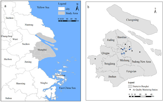
Figure 1.
Map of the study area: (a) Location of Shangai in the Yangtze River Delta. (b) Location of state-monitored air quality stations. A is Jing’an monitoring station. B is Shanghai Normal University monitoring station. C is Pudong monitoring station.
In 2020, COVID-19 was deemed a pandemic, resulting in restrictions on economic activity and changes in human behavior. Air quality improvements were observed in Shanghai due to pollution prevention and control, with lockdown measures being enforced to limit the spread of COVID-19. In 2020, the annual average PM2.5 concentration in the ambient air was 32 μg/m3 in Shanghai, a record low since monitoring began. To investigate the impact of the COVID-19 pandemic on air quality, the hourly time series data of PM2.5 concentrations measured by 10 state-monitored air quality stations, and meteorological observations that are measured by 10 state-monitored weather stations, are collected. Among the 10 air quality monitoring stations, nine stations are located in the downtown area, except the Dianshan Lake monitoring station in the Qingpu District. In addition to the monitoring data, thematic maps related to land use, road network, and functional areas are used to investigate the characteristics and geographic origins of emission sources.
3. Methodology
3.1. Construction of Bivariate Polar Plots
Firstly, a speed–wind direction polar coordinate system is established. Using the time series data of PM2.5 concentration, wind speed, and wind direction, a Generalized Additive Model (GAM) is applied to construct the bivariate polar plots by fitting the numerical surfaces between wind vectors and PM2.5 concentrations. Then, the variation of pollutant concentrations with meteorological conditions such as wind speed and wind direction can be shown in polar coordinates. The specific steps to construct the bivariate polar plots are as follows [11]:
Based on wind direction interval at 10° and wind speed interval at 30 m/s, multiple two-dimensional bins composed of wind direction and speed are generated. Each set of monitoring data, including the hourly wind direction, wind speed, and PM2.5 concentration at each monitoring site, are partitioned into the corresponding bins. The mean PM2.5 concentration (C) falling in each bin is calculated.
According to wind speed and direction, two components of wind vector, u and v, are calculated, i.e.,
where is the mean hourly wind speed in each bin, and is the mean wind direction in degrees with 90° as being from the east.
The GAM is applied to fit u, v, and concentration (C) surfaces to construct bivariate polar plots in order to describe the variation of PM2.5 concentration (C) as a function of the wind components u and v. The GAM can be expressed as shown in Equation (2):
where Ci is the ith PM2.5 concentration data, β0 is the intercept of the model, s(ui, vi) is the isotropic smooth function of the ith value of covariant u and v, and εi is the ith residual. A penalized regression spline is used to model the surface.
Bivariate polar plots provide an effective graphical method for identifying air pollutant sources and describing the characteristics of emission sources rather than noise.
3.2. Cluster Analysis
Cluster analysis groups data objects into a certain number of classes based on the similarity between objects, so that the objects with a higher similarity are classified into the same class. The indicators, such as distance and density, are usually adopted to evaluate the similarity. There are two types of classical algorithms based on the distance measure, namely, the Partitioning Method and Hierarchical Method, of which the k-means and k-medoids algorithms are typical representatives. After inputting the number of classes (K), the k-means algorithm partitions the n data objects into K classes, so that the data points in each class have the shortest distance from the center of the class.
The three variables used to calculate the similarity in cluster analysis are the wind components u and v and the PM2.5 concentration (C). The data of all three variables should be standardized first because the wind components u and v are on different scales to C. In the k-means clustering algorithm, the n data objects X = {xi}, i = 1, …, n, are divided into K classes, i.e., C = {ck, k = 1, …, K}. The iterations can be terminated when the calculation result of the formula reaches a minimum value, wherein represents a chosen distance measure and μk is the mean of data objects in class ck. In this paper, the Euclidean distance is used to calculate the distance between data:
where x and y are J-dimensional vectors, which is the set of standardized values of u, v, and PM2.5 concentration, and J is of length three.
The bivariate polar plot features can be effectively identified and grouped by using the k-means algorithm, and, moreover, different emission sources can be automatically partitioned.
3.3. Detection of Source Directions and Geographic Origins
According to the clustering results, the time series data of PM2.5 concentrations for each cluster are extracted and analysed for further accurate acquisition of source characteristics and quantification of source contributions. The temporal variations in concentration by cluster could help determine the source types represented by each cluster. Furthermore, meteorological data and thematic maps of land use, road network, and functional areas are adopted to reveal the main factors related to meteorological conditions and anthropogenic activity influencing the emission and dispersion of a fine particulate pollutant. The results of source apportionment combined with land use, wind speed, and direction data are used to locate the most possible directions of different source categories and geographic origins of PM2.5 and to assess the impacts of local emissions and regional transport on the accumulation of fine particulate matter.
4. Results
4.1. Temporal Variation in PM2.5 Concentration
4.1.1. Seasonal Variation in PM2.5 Concentration
Based on the air quality monitoring data, the PM2.5 concentrations in Shanghai are significantly higher in winter than in summer. Indeed, the PM2.5 concentrations change in the order of winter > spring > autumn > summer (Figure 2). January and December are the coldest months, when the increased use of heating equipment, such as air conditioners and electric heaters, results in a rise in electricity consumption. In winter, precipitation is low, and winds prevail in the northwest direction. Therefore, fine particulate pollutants from the inland area accumulate in Shanghai, downwind of the prevailing wind direction. Given the above, the PM2.5 concentrations are the highest in these two months. The air temperature begins to rise continuously since May, and the atmospheric convection intensifies, which is conducive to the dispersion of fine particulate matter. Moreover, the precipitation becomes more frequent between June and September, facilitating the dilution and clearance of particulate pollutants. Therefore, the monthly average PM2.5 concentrations in summer and autumn are the lowest within a year.
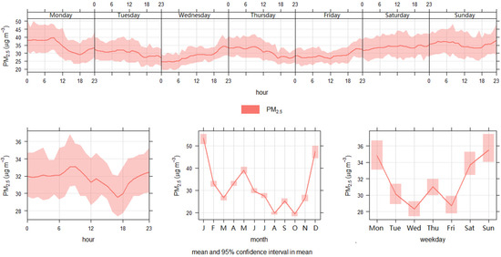
Figure 2.
Temporal variation in PM2.5 concentration in Shanghai.
4.1.2. Weekly Variation in PM2.5 Concentration
The weekly variation in PM2.5 concentration shows that the PM2.5 concentrations are relatively higher on Mondays and weekends. No significant weekend effects are observed in fine particulate pollution. The PM2.5 concentrations are generally higher on weekends than those in midweeks, indicating that the changes in the daily activities on weekends have a negative impact on air quality. This finding is consistent with that attained by other scholars [13]. A large number of production activities continue on weekends. In addition, more people choose private cars for travel than on weekdays, and larger traffic volume undoubtedly makes traffic-related emissions more serious.
4.1.3. Hourly Variation in PM2.5 Concentration
Morning rush hour is the time with a sudden surge in traffic flow, accompanied by an increase in the anthropogenic emissions of fine particulate matter. Moreover, the air temperature is generally lower in the morning, as is the height of the atmospheric mixed layer. A temperature inversion is more likely to form in the near-surface atmosphere in the morning, which is not conducive to pollutant dispersion. For this reason, the first peak of PM2.5 concentration occurs. The travel activities are reduced around noon, resulting in a reduction in traffic-related emissions. Meanwhile, the convective activity is enhanced in the atmosphere, promoting pollutant dispersion and a gradual decrease in PM2.5 concentration in the afternoon. Toward the evening, rush hour brings a rise in traffic-related pollution, and cooking-related pollution is also observed, leading to a gradual increase in PM2.5 concentration. At midnight, the price of industrial electricity is at the low stage, according to the tiered pricing scheme, and the intensive operations of many factories cause continuous industrial emissions. Therefore, the PM2.5 concentrations from midnight to dawn remain at a relatively higher level.
As shown in Figure 3, the peak of daily PM2.5 concentration occurs from 6:00 to 8:00 am, while its trough occurs from 15:00 to 18:00 p.m. in summer (June to August). Changes in anthropogenic emission sources and boundary layer height will cause daily variation of PM2.5 concentrations in summer. Morning rush hour is from 6:00 to 8:00 a.m. when the PM2.5 concentrations increase significantly, accompanied with a sharp increase in vehicle exhaust emissions. Moreover, the daytime air temperature and humidity are usually higher in summer. The photochemical reaction is of higher intensity in the atmosphere, which is very likely to result in the generation of secondary aerosol (mainly fine particulate matter).
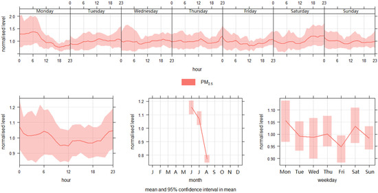
Figure 3.
Temporal variation in PM2.5 concentration in Shanghai in summer.
In winter (January and February), the PM2.5 concentration reaches its second peak between 19:00 and 21:00 p.m., indicating that the pollution sources change from road traffic to domestic activity (Figure 4). Home heating by residents in winter is an important source of PM2.5 emissions, and volatile substances condense in the nighttime, resulting in fine particulate matter. In addition, a large number of air pollutants are generated around dawn due to industrial production and construction activities that begin at this time of the day.
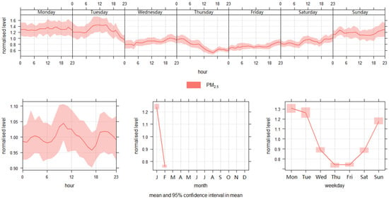
Figure 4.
Temporal variation in PM2.5 concentration in Shanghai in winter.
4.2. Bivariate Concentration Polar Plot
Using the hourly time series data from nine air quality monitoring stations in the downtown area, the bivariate polar plot is developed to investigate the non-linear relationship between PM2.5 concentrations and wind speeds and directions, and to visualize the transport pathways from different emission sources in the winter of 2020 (January and February).
According to Figure 5, a high PM2.5 concentration region along the northwest direction is prominently shown in the bivariate polar plot. Under the wind prevailing in the northwest direction in winter (see Figure 6), regional scale transport of air pollutants from external sources, accompanied by emissions from industrial activities in the Baoshan and Jiading districts, such as road traffic and domestic gas combustion, results in the accumulation of fine particulate matter in this direction. Moreover, high concentrations of PM2.5 are mostly attributed to low wind speed conditions when weak winds prevail along the southwest and northeast directions. In these wind directions, the PM2.5 concentration decreases as the wind speed increases. High PM2.5 concentrations distributed near the plot center are related to local emission sources from the intertwining road network, home heating, and cooking. However, the inverse relationship between wind speeds and PM2.5 concentrations is not obvious in the southeast of the bivariate polar plot, which can be explained by the emissions from the industrial zones, ports, and Shanghai Pudong International Airport in southeastern Shanghai.
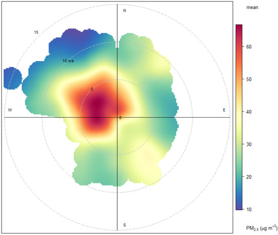
Figure 5.
Bivariate polar plot of PM2.5 concentrations in Shanghai in the winter of 2020. The radial axis is wind speed in m s−1 and the colour scale is the concentration of PM2.5 in µg m−3.
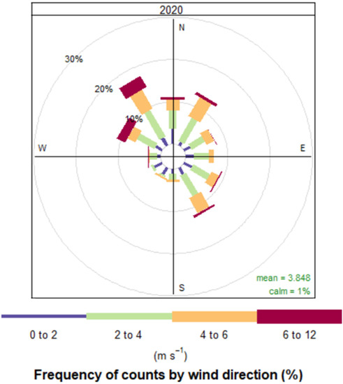
Figure 6.
Wind rose showing the wind speed and direction frequencies in Shanghai in the winter of 2020.
4.3. PM2.5 Source Characteristics in Shanghai
The k-means method is used to perform a clustering analysis on the result of the bivariate polar plot. Combined with the temporal variation analysis for the clusters, different emission sources of PM2.5 are distinguished, and the mean concentration and contribution of each source type are calculated.
Figure 7 shows the clustering results for the wintertime PM2.5 surface (see Figure 5) using the k-means method, ranging from a two-cluster to a ten-cluster solution. After grouping the features observed on the bivariate concentration polar plot using the solutions, it is identified that the eight-cluster solution is appropriate for discriminating the emission sources. To further illustrate the temporal variation in concentrations by cluster, the hourly, daily, and weekly variation plots of the eight subsets are given in Figure 8.
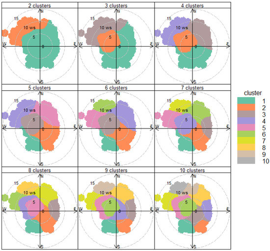
Figure 7.
Clusters identified for PM2.5 concentrations for 2 to 10 clusters.
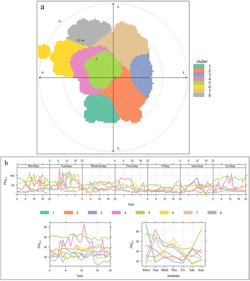
Figure 8.
Temporal variation in PM2.5 concentration for the eight-cluster solution: (a) Eight-cluster solution obtained on PM2.5 bivariate concentration polar plot. (b) Hourly, daily, and weekly variation of eight clusters. The vertical axis is the concentration of PM2.5 in µg m−3.
Clusters 2, 4, 5, and 7 appear every day from Monday to Sunday with a clear feature of continuous hourly variation. According to the transport directions of fine particulate matter shown in Figure 5, Cluster 2 mostly represents the emission sources from the industrial zones, ports, and Shanghai Pudong International Airport in southeastern Shanghai. When compared with the hourly variation of concentrations in Clusters 4 and 5, Cluster 4 mostly represents the sources from industrial zones in the Baoshan, Jiading, Songjiang, and Minhang districts, while Cluster 5 mostly represents local sources related to traffic and biomass burning for home heating and cooking. In addition, the temporal variation of concentrations in Cluster 7 reveals an increase during the period from afternoon to night, indicating that Cluster 7 is dominated by the source related to the operation of ports in northeastern Shanghai. Consequently, Clusters 2, 4, 5, and 7 are identified as local sources. On the other hand, Clusters 1, 3, 6, and 8, appearing occasionally in a week with different lengths of occurrence each day, are observed for high wind speeds, typically >about 5 m s−1; thus, they are considered as external sources that are transported from the southwest, east, and northwest directions, respectively. The average concentration of the data falling into Clusters 1, 3, 6, and 8 has been found to be 24.34 µg/m3 for PM2.5, while the average concentration of the data in Clusters 2, 4, 5, and 7, was 46.56 µg/m3 for PM2.5. Therefore, it is estimated that the contribution of external sources of PM2.5 accounts for 34.33% and the contribution of local sources accounts for 65.67% in Shanghai in the winter of 2020.
4.4. Spatial Heterogeneity of PM2.5 Emission Sources
Our previous study demonstrates that the spatial distribution of PM2.5 concentrations in Shanghai is different from the ‘downtown–downtown edge–suburban’ decreasing trend observed in other cities. Instead, Shanghai exhibits the ‘suburban, non-suburban’ mode, indicating that Shanghai has multiple regions of high PM2.5 emissions in the downtown area [14]. Therefore, in this study, three monitoring stations, including the Jing’an monitoring station (31°13′ N, 121°25′ E) in the Jing’an District, the Shanghai Normal University monitoring station (31°10′ N, 121°25′ E) in the Xuhui District, and the Pudong monitoring station (31°14′ N, 121°32 ′E) in the Pudong New Area, are selected to perform further analyses on the spatial heterogeneity of PM2.5 emission sources in Shanghai.
4.4.1. Jing’an Monitoring Station
The Jing’an monitoring station is located in a central business area and is surrounded by high and low buildings. The complex street canyons cause significant local variation in the dispersion and distribution of PM2.5. This area is characterized by dense road network, heavy traffic, and land shortage. Its complex transportation microenvironment is formed by roads, overpasses, and elevated highways, and traffic-related emissions lead to the accumulation of fine particulate matter under low wind speeds. A region with high PM2.5 concentrations in the northwest of the bivariate polar plot (Figure 9) corresponds to industrial activities in the Baoshan District bordering on the Jing’an District and transport of pollutants from external sources. High PM2.5 concentrations under low wind speeds in the southwest are related to large-scale business circles and densely distributed traffic arteries. In addition, the PM2.5 concentrations at the station are also affected by the emission sources from Shanghai Railway Station in the northeast direction and from the industrial zones, airport, and ports in the Pudong New Area bordering on the Jing’an District in the southeast.
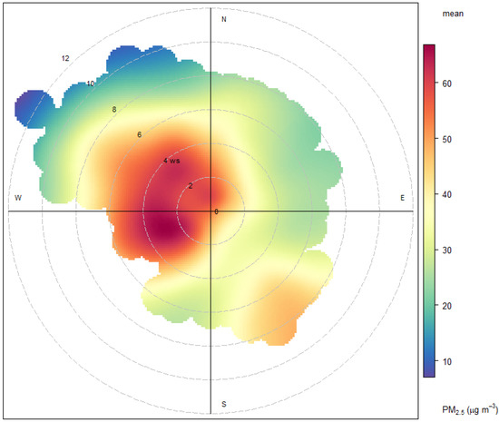
Figure 9.
Bivariate polar plot of PM2.5 concentrations at the Jing’an monitoring station.
4.4.2. Shanghai Normal University Monitoring Station
Figure 10 shows the bivariate concentration polar plot for PM2.5 at the Shanghai Normal University monitoring station. High PM2.5 concentrations are found in the northwest of the plot, revealing the accumulation of fine particulate pollutants by the effect of local sources under low wind speed conditions, as well as regional scale transport under higher wind speed conditions. In terms of the functional areas and land use types around this monitoring station, the local sources in the northwest direction are likely related to industrial activities at Caohejing Development Zone and Qingpu Industrial Zone, and traffic emissions from Hongqiao Transport Hub, which includes Hongqiao Railway Station and Hongqiao Airport. On the other hand, the accumulation of fine particulate matter also occurs in the southwest of the plot. This is related to traffic emissions from the elevated roads and the Shanghai South Railway Station. As the third largest railway station in Shanghai, Shanghai South Railway Station acts as an important transportation hub that includes the railway station and the long-distance bus station.
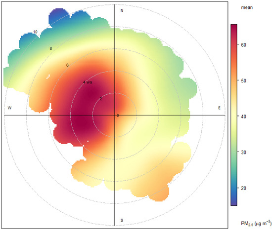
Figure 10.
Bivariate polar plot of PM2.5 concentrations at the Shanghai Normal University monitoring station.
4.4.3. Pudong Monitoring Station
Figure 11 shows the bivariate polar plot for PM2.5 concentrations at the Pudong monitoring station. High PM2.5 concentrations occurring under low wind speed conditions from the northwest, southwest, and northeast are related to local industrial activities and vehicle exhaust emissions. However, the wind speeds of the northwest wind are observed to be relatively higher at the Pudong monitoring station than those of the other stations in the downtown area. In addition to traffic-related emissions, distant, large-point sources, such as the Baoshan steelworks and industrial zones in the Baoshan and Jiading districts, also aggravate the air pollution in the northwest direction. Moreover, Shanghai South Railway Station and industrial zones in the Minhang District in the southwest, Pudong International Airport in the southeast, and the ports along the coast of the East China Sea also contribute to air pollution at this monitoring station.
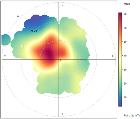
Figure 11.
Bivariate polar plot of PM2.5 concentrations at the Pudong monitoring station.
5. Discussion
At the end of 2019, the novel coronavirus (COVID-19) epidemic broke out in Wuhan and spread around the whole of China in 2020. In order to prevent the spread of COVID-19, a series of mandatory actions have been taken by the municipal and provincial governments, such as measures to restrict travel across cities, production, and business. However, Shanghai was only slightly affected by the epidemic in 2020, and its prevention and control measures were also relatively permissive compared with Wuhan, and human behavior and economic activity remained almost unchanged. Our results show that the factors influencing the PM2.5 concentrations in the downtown area of Shanghai are related to meteorological conditions, regional scale transport of fine particulate pollutants from external sources, and local emission sources, including traffic, industrial activities, biomass burning for home heating and cooking, etc. Vehicle exhaust emissions on roads, vessels’ exhaust emissions at ports, inland waterway transport emissions, and fuel burning in airplanes and non-road mobile machinery constitute traffic-related emissions of PM2.5. The growth of motor vehicle ownership, a sprawling transport network, severe traffic jams, and a large volume of travel and freight transport in Shanghai result in a higher level of PM2.5 concentrations on weekends than during midweeks. Coal-burning activities in Shanghai are most intensive in the power industry. There is no collective heat supply in winter, and coal burning is dispersed. Therefore, the contribution of coal burning to PM2.5 emissions in Shanghai is significantly less than that in the northern cities in China. However, industry is an integral part of Shanghai’s industrial structure, which is featured by a great diversity of subsectors and huge volumes of production economies and energy consumption. Industrial production is still a primary source of PM2.5 emissions in Shanghai.
Studies on several consecutive severe PM2.5 pollution events in Shanghai have demonstrated that the atmospheric environment is influenced by the regional scale transport of air pollutants from the Yangtze River Delta, the Central Plains, the inland area of northern China, and coastal cities in the north and south of Shanghai [15,16]. Transported by air mass at low speeds, a large amount of air pollutants from industrial sources in the Yangtze River Delta and coastal cities in the north and south of Shanghai result in the accumulation of air pollutants. In addition, dust from sandstorm-prone areas in northern China usually causes dust storm pollution in Shanghai. Because dust can absorb and carry coal-fired organic pollutants, the mix and interaction between dust and coal-fired pollutants will exert a significant impact on air quality in downwind areas [17].
In calm weather in winter, a full mix of water vapour in marine air mass and fine particulate matter will exacerbate the secondary formation of fine particulate matter and become one major transport pathway of fine particulate matter. The PM2.5 concentrations and PM2.5/PM10 ratio under the influence of the eastern marine air mass are very high, which is probably due to the high vapor content and stable atmospheric conditions that are favorable for secondary formation [18].
During the COVID-19 lockdown period, industrial activities in different regions were limited to varying degrees, resulting in the reduction in the emissions of industrial pollutants and fumes. However, in January and February 2020, the unfavorable meteorological conditions (the high relative humidity, low wind speeds, and boundary layer height) in northern China promoted the formation of secondary aerosols via multiphase reactions, causing the severe haze pollution in northern China, further contributing to the change in PM2.5 concentration in Shanghai.
There are some limitations in this study that could be addressed in future research. First, this study focuses on the characterization of PM2.5 emission sources in Shanghai during the COVID-19 outbreak. Future studies will assess the impact of changes in human activities related to compound air pollution, which is dominant in most Chinese cities, by using the time series concentration data of other pollutants, such as NO2, SO2, CO, and O3. Moreover, the study area will not be confined to Shanghai, but expanded to the Yangtze River Delta and Wuhan City Circle. Although the bivariate concentration polar plots can be used to understand the emission source characteristics, this method cannot reveal the process and trajectory of regional scale transport of air pollutants, which will be investigated by calculating and clustering back trajectories.
6. Conclusions
Bivariate polar plots provide an effective graphical method for visualizing the relationship between PM2.5 concentrations and meteorological parameters, identifying air pollutant sources and describing the characteristics of emission sources rather than noise. This study uses bivariate concentration polar plots, combined with k-means clustering and temporal variation analyses for PM2.5 time series data, to understand the PM2.5 source characteristics in Shanghai during COVID-19 pandemic in the winter of 2020. Our findings show that 34.33% of the PM2.5 particles arise from external sources while 65.67% are from local sources (mainly traffic, industry activities and biomass burning). The results of source apportionment combined with land use, wind speed, and direction data are further used to locate the most possible directions of different source categories and geographic origins of PM2.5.
In spite of the lockdown measures to limit the spread of COVID-19, Shanghai was slightly affected by the epidemic. Thus, human behavior and economic activity experienced little change in 2020. Traffic and industrial activity are still primary local sources of PM2.5 emissions in Shanghai. Meanwhile, regional scale transport of air pollutants from the Yangtze River Delta, the Central Plains, the inland area of northern China, and coastal cities north and south of Shanghai aggravate the air pollution in Shanghai under unfavorable meteorological conditions. Our future work will focus on the impact of the COVID-19 pandemic on the variations of PM2.5 emission sources in the following years, due to the reduction in the international logistics transportation and the production of export processing enterprises as a result of widespread restrictions on economic activity around the world.
Author Contributions
X.D. proposed the methodology, data calculation and result analysis. The C.W., L.Z. and P.L. contributed to the data collection, analysis, and discussion. All authors have read and agreed to the published version of the manuscript.
Funding
This study is financially supported by the National Natural Science Foundation of China [No. 41501508 & 41801246], and Zhejiang Province Public Technology Research Projects (LGF18C030001).
Data Availability Statement
Time series data of PM2.5 concentrations come from the National Urban Air Quality Real-Time Release Platform of China National Environmental Monitoring Center (https://air.cnemc.cn:18007/). Meteorological observation data come from National Climatic Data Center (ftp://ftp.ncdc.noaa.gov/pub/data/noaa/isd-lite/). All website accessed on 29 July 2022.
Conflicts of Interest
The authors declare no conflict of interest.
References
- Lin, Y.L.; Zou, J.L.; Yang, W.; Li, C.Q. A Review of Recent Advances in Research on PM2.5 in China. Int. J. Environ. Res. Public Health 2018, 15, 438. [Google Scholar] [CrossRef] [PubMed]
- He, K.B.; Yang, F.M.; Duan, F.K.; Ma, Y. Atmospheric Particulate Matter and Regional Complex Pollution; Science Press: Beijing, China, 2011. [Google Scholar]
- Hopke, P.K.; Dai, Q.; Li, L.; Feng, Y. Global Review of Recent Source Apportionments for Airborne Particulate Matter. Sci. Total Environ. 2020, 740, 140091. [Google Scholar] [CrossRef] [PubMed]
- Ali-Taleshi, M.S.; Moeinaddini, M.; Bakhtiari, A.R.; Feiznia, S.; Squizzato, S.; Bourliva, A.A. One-Year Monitoring of Spatiotemporal Variations of PM2.5-bound PAHs in Tehran, Iran: Source Apportionment, Local and Regional Sources Origins and Source-Specific Cancer Risk Assessment. Environ. Pollut. 2021, 274, 115883. [Google Scholar] [CrossRef] [PubMed]
- Chen, R.; Jia, B.; Tian, Y.; Feng, Y. Source-Specific Health Risk Assessment of PM2.5-Bound Heavy Metals Based on High Time-Resolved Measurement in a Chinese Megacity: Insights into Seasonal and Diurnal Variations. Ecotoxicol. Environ. Saf. 2021, 216, 112167. [Google Scholar] [CrossRef] [PubMed]
- Song, Y.; Huang, B.; He, Q.; Chen, B.; Wei, J.; Mahmood, R. Dynamic Assessment of PM2.5 Exposure and Health Risk Using Remote Sensing and Geo-Spatial Big Data. Environ. Pollut. 2019, 253, 288–296. [Google Scholar] [CrossRef] [PubMed]
- Liang, C.S.; Yue, D.; Wu, H.; Shi, J.S.; He, K.B. Source Apportionment of Atmospheric Particle Number Concentrations with Wide Size Range by Nonnegative Matrix Factorization (NMF). Environ. Pollut. 2021, 289, 117846. [Google Scholar] [CrossRef] [PubMed]
- Zhou, M.; Jiang, W.; Gao, W.; Gao, X.; Ma, M.; Ma, X. Anthropogenic Emission Inventory of Multiple Air Pollutants and Their Spatiotemporal Variations in 2017 for the Shandong Province, China. Environ. Pollut. 2021, 288, 117666. [Google Scholar] [CrossRef] [PubMed]
- Elangasinghe, M.A.; Singhal, N.; Dirks, K.N.; Salmond, J.A.; Samarasinghe, S. Complex Time Series Analysis of PM10 and PM2.5 for a Coastal Site Using Artificial Neural Network Modelling and K-Means Clustering. Atmos. Environ. 2014, 94, 106–116. [Google Scholar] [CrossRef]
- Carslaw, D.C.; Beevers, S.D.; Ropkins, K.; Bell, M.C. Detecting and Quantifying Aircraft and Other on-Airport Contributions to Ambient Nitrogen Oxides in the Vicinity of a Large International Airport. Atmos. Environ. 2006, 40, 5424–5434. [Google Scholar] [CrossRef]
- Carslaw, D.C.; Beevers, S.D. Characterising and Understanding Emission Sources Using Bivariate Polar Plots and K-Means Clustering. Environ. Model. Softw. 2013, 40, 325–329. [Google Scholar] [CrossRef]
- Hui, L.; Ma, T.; Gao, Z.; Gao, J.; Wang, Z.; Xue, L.; Liu, H.; Liu, J. Characteristics and Sources of Volatile Organic Compounds during High Ozone Episodes: A Case Study at a Site in the Eastern Guanzhong Plain, China. Chemosphere 2021, 265, 129072. [Google Scholar] [CrossRef] [PubMed]
- Li, M.S.; Ren, X.X.; Yu, Y.; Zhou, L. Spatiotemporal Pattern of Ground-Level Fine Particulate Matter (PM2.5) Pollution in Mainland China. China Environ. Sci. 2016, 36, 641–650. [Google Scholar]
- Chen, C. Spatial Distribution Characteristics of Atmospheric Particulate Pollution and its Influential Factors: Study on Shanghai at Different Scales. Master’s Thesis, Fudan University, Shanghai, China, 2018. [Google Scholar]
- Zhou, M.; Qiao, L.P.; Zhu, S.H.; Li, L.; Lou, S.R.; Wang, H.L.; Tao, S.K.; Huang, C.; Chen, C.H. Chemical Characteristics of Particulate Matters and Trajectory Influence on Air Quality in Shanghai during the Heavy Haze Episode in December, 2013. Environ. Sci. 2016, 4, 1179–1187. [Google Scholar]
- Long, S. Characteristics of Major Physical and Chemical Processes during Haze Day in Shanghai. Ph.D. Thesis, University of Chinese Academy of Sciences, Shanghai, China, 2014. [Google Scholar]
- Wei, X.; Zhang, R.; Zhuang, G.S. The Impact of Coal-fired Pollutants through Long-Range Transport on Air Quality. J. Fudan Univ. 2011, 50, 547–555. [Google Scholar]
- Zhu, S.H.; Zhou, M.; Qiao, L.P.; Li, L.; Lou, S.R.; Yan, R.S.; Wang, H.L.; Tao, S.K.; Chen, C.H. Impact of the air Mass Trajectories on PM2.5 Concentrations and Distribution in the Yangtze River Delta in December 2015. Acta Sci. Circumstantiae 2016, 36, 4285–4294. [Google Scholar]
Publisher’s Note: MDPI stays neutral with regard to jurisdictional claims in published maps and institutional affiliations. |
© 2022 by the authors. Licensee MDPI, Basel, Switzerland. This article is an open access article distributed under the terms and conditions of the Creative Commons Attribution (CC BY) license (https://creativecommons.org/licenses/by/4.0/).