Abstract
Carbon emissions and consequent climate change directly affect the sustainable development of ecological environment systems and human society, which is a pertinent issue of concern for all countries globally. The construction of a carbon emission inversion model has significant theoretical importance and practical significance for carbon emission accounting and control. Established carbon emission models usually adopt socio-economic parameters or energy statistics to calculate carbon emissions. However, high-precision estimates of carbon emissions in administrative regions lacking energy statistics are difficult. This problem is especially prominent in small-scale regions. Methods to accurately estimate carbon emissions in small-scale regions are needed. Based on nighttime light remote-sensing data and the STIRPAT (Stochastic Impacts by Regression on Population, Affluence, and Technology) model, combined with the environmental Kuznets curve, this paper proposes an ISTIRPAT (Improved Stochastic Impacts by Regression on Population, Affluence, and Technology) model. Through the improved STIRPAT model (ISTIRPAT) and panel data regression, provincial carbon emission inventory data were downscaled to the municipal level, and municipal scale carbon emission inventories were obtained. This study took the 17 cities and prefectures of Hubei Province, China, as an example to verify the accuracy of the model. Carbon emissions for 17 cities and prefectures from 2012 to 2018 calculated from the original STIRPAT model and the ISTIRPAT model were compared with real values. The results show that using the ISTIRPAT model to downscale the provincial carbon emission inventory to the municipal level, the inversion accuracy reached 0.9, which was higher than that of the original model. Overall, carbon emissions in Hubei Province showed an upward trend. Regarding the spatial distribution, the main carbon emission area was formed in the central part of Hubei Province as a ring-shaped mountain peak. The lowest carbon emissions in the central area expanded outward, increased, and gradually decreased to the edge of the province. The overall composition of carbon emissions in eastern Hubei was higher than those in western Hubei.
1. Introduction
Climate change has become an important challenge globally for sustainable development. Calculating and controlling carbon emissions is a critical issue of concern for the international community. Since the industrial revolution, the extensive use of energy sources, such as oil and coal, has increased carbon dioxide emissions annually. Currently, 178 Parties worldwide have signed the Paris Agreement aimed at addressing climate change. China, the United States of America, the European Union (including the United Kingdom), India, Russia, and Japan are the six major greenhouse gas emitters (regions), as per UNEP (United Nations Environment Programme) data. These countries accounted for 62.5% of the global carbon emissions in the last decade (2010–2019). As a developing country, China accounted for 26.7% of global carbon emissions in 2019. In 2020, China proposed that carbon dioxide emissions should peak by 2030, and it endeavored to implement carbon neutralization (carbon neutrality) by 2060. Therefore, accurate accounting of carbon emissions at different scales has reference value and guiding significance for the implementation of regional carbon emission policies and the achievement of the ‘Carbon peaking and carbon neutrality goals’.
Extensive studies have been focused on the accounting and prediction of carbon emissions, and these can be divided into three categories: influencing factor decomposition method, regression analysis method, and energy statistics method [1]. Among the decomposition methods of influencing factors, the most representative one is the logarithmic Divish index model (LMDI). Using spatial and temporal dimensions, the LMDI model decomposes carbon emissions as targets to form multiple single influencing factors for calculating the contribution of a particular factor toward changing carbon emissions over time [2,3]. As per the spatial and temporal characteristics of the LMDI model, historical and predicted carbon emissions can be decomposed, and regional carbon emissions can be predicted and affected by population, industry, and other factors [4,5]. Regression analysis methods include the IPAT (Impact, Population, Affluence, Technology) model, its extended STIRPAT (Stochastic Impacts by Regression on Population, Affluence, and Technology) model, OLS (Ordinary Least Squares) regression model, and neural network algorithms [6,7]. For example, only the STIRPAT model [8,9,10,11], or the combination of neural network and STIRPAT model [12], is used for predictions, and the improved IPAT model is used to simulate and predict future urban development [13,14,15,16,17,18,19]. Energy statistics methods can be divided into two types: carbon emission statistics based on production and consumption [20]. The former has been used to calculate carbon emissions from domestic production and export products, mainly considering the carbon emissions at the production point but not considering those created by users and at usage places [21,22]. The latter is an assessment of carbon emissions from end-of-life consumption activities, mainly applied to national and urban carbon emission calculations [23,24,25]. Irrespective of the method, few studies have focused on carbon emissions accounting at a small spatial scale due to the requirement for highly detailed energy statistics.
In recent years, the scale of carbon emission calculations has gradually shifted to municipal and county levels [26,27]. However, the current method model is only established for specific regions, and it cannot be applied in other regions. Whether it is through land-use data to obtain carbon emissions [28] or proportionally allocate provincial carbon emissions to the municipal level [29], the factors affecting carbon emissions considered in these approaches are not comprehensive, resulting in large errors in the carbon emission accounting process. Nighttime lighting data have been widely used to simulate socio-economic conditions as the intensity of night lighting can be used to indicate energy consumption level [30,31]. These data are typically evaluated by linear, exponential, logarithmic, and quadratic polynomial simulation, and panel data regression is the most effective method [32,33,34]. These methods to obtain carbon emissions are based only on remote-sensing data without incorporating multi-source social data, making it difficult to identify social factors that have important impacts on carbon emissions.
Energy statistics can be used for national or provincial carbon emission accounting; however, this approach has various issues, such as missing data and inconsistent statistical caliber for municipal carbon emission accounting [35,36]. The efficient and accurate estimation of carbon emissions at a small scale is a key issue in achieving regional sustainable development under carbon emission targets. In this paper, an improved STIRPAT carbon emission inversion model (ISTIRPAT) is proposed based on the city development element (CDE) constructed using NPP/VIIRS (National Polar-Orbiting Partnership/Visible Infrared Imaging Radiometer Suite) nighttime lighting data. The provincial carbon emission inventory was downscaled to the municipal level by panel regression and the ISTIRPAT model. Hubei Province was taken as an example to verify the inversion accuracy of the model. Carbon emissions and spatiotemporal patterns were analyzed for 17 cities and prefectures in Hubei Province from 2012 to 2018. This paper provides an improved model (ISTIRPAT) that can downscale carbon emissions from large-scale regions to small-scale regions, and it addresses the lack of energy statistics at small scale in various countries or regions and is expected to contribute to the accounting of carbon emissions at a small scale.
2. Study Area and Data
2.1. Study Area
Hubei Province is located in eastern China, between 29°01′53″–33°6′47″ N and 108°21′42″–116°07′50″ E (Figure 1). The province spans 740 km in the east-west direction and approximately 470 km in the north-south direction, with a total area of 185.9 million sq km, accounting for 1.94% of the total area of China. By 2020, Hubei Province had jurisdiction over 12 prefecture-level cities, 1 autonomous prefecture, 26 county-level cities, 35 counties, 2 autonomous counties, and 1 forest area, with a permanent population of 57.75 million and GDP of CNY 434.4346 million. Among them, the values added for primary, secondary, and tertiary industries are CNY 413.191, 172.390, and 222.8765 billion, respectively.
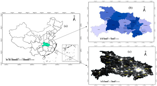
Figure 1.
Overview of Hubei Province: (a) Location of Hubei Province; (b) Hubei’s topography and 17 cities; (c) Nightlight remote-sensing data for Hubei Province, 2015.
Hubei Province, the central region of the Yangtze River Economic Belt, plays an important role in the transportation hub. It is dependent on the Yangtze River Basin and is located in an urban agglomeration in the middle of the Yangtze River. It has become an important strategic area for economic development in the development pattern of ‘one axis, two wings, three levels and multiple points’ of the Yangtze River Economic Belt [37]. However, the infrastructure construction level in Hubei Province is not balanced, resource integration is insufficient, and environmental protection is under significant pressure. Hubei is mainly a heavy industrial area, with many energy-intensive industries, such as steel, shipbuilding, and chemical industries. Carbon emissions have gradually increased with the development of industry and increasing energy consumption. From 2001, after China became a member of the WTO (World Trade Organization), carbon emissions in the province increased from 126.84 million tons to 322.37 million tons in 2018, with an annual growth rate of 11.5018 million tons [38].
2.2. Data Sources
Provincial carbon emission inventories and carbon emission inventories for 17 administrative regions of Hubei Province were obtained from the dataset released by CEADs (https://www.ceads.net.cn/, accessed on 20 September 2021), China Carbon Accounting Database. The nighttime lighting remote-sensing data NPP/VIIRS is a Beta1 dataset for 2012 to 2018 for China provided by the Aerospace Information Research Institute, Chinese Academy of Sciences (https://www.zybuluo.com/novachen/note/1741875, accessed on 19 August 2021). The nighttime light remote-sensing images had a resolution of 1500 m, which is 0.0125 degrees per pixel (28,800 × 11,200 pixels). The nighttime light remote-sensing images were preprocessed, and DN values were normalized in the range of 0–256. Provincial statistics for China were obtained from the National Statistical Yearbook (http://www.stats.gov.cn/, accessed on 18 September 2021). The statistical data for the cities in Hubei Province were obtained from the Statistical Yearbook of Hubei Province (http://tjj.hubei.gov.cn/, accessed on 9 October 2021). The provincial carbon emission inventories for 2012–2018 obtained from the CEADs database were used as training sets, and the carbon emission inventories of 17 cities and prefectures in Hubei Province from 2012 to 2017 obtained from the CEADs database were used as the verification set.
3. Methods
3.1. Extension of the STIRPAT Model
As one of the environmental impact factor models, IPAT and extended models based on IPAT have been widely used to analyze the impact of socio-economic factors on pollutant emissions. However, the model needs to unify the dimensions of environmental impact factors and cannot accurately reflect the impact on the environment when the influencing factors change. Dietz improved the IPAT model and proposed a random regression model known as STIRPAT [39] (Formula (1)).
The basic formula of the STIRPAT model is as follows:
where I, P, A, and T represent the environmental conditions, population, economic development, and technological innovation, b, c, and d are the estimation coefficients of the three driving factors, denotes the model parameter, and indicates the error term. Therefore, in this paper, environmental condition represents carbon emission , its driving factor represents the population , A represents gross domestic product (, and represents the added value of the secondary industry . Carbon emissions mainly involve energy combustion in the cement industry, and energy is mainly related to the use of coal, diesel, and other combustion materials. The use of these fuels is closely linked with the production in heavy, light, and manufacturing industries in cities. Data acquisition for the cement industry is difficult at the municipal level. However, for the cement industry production and consumption, construction industry becomes the main component, and most cement consumption takes place at the construction site. Therefore, in this paper, adding the total value of the secondary and construction industries into the model, the basic formula for the STIRPAT model for carbon emissions is obtained, as shown in Formula (2).
The Kuznets curve was proposed and used by Nobel Prize winner Simon Smith Kuznets in the 1950s to analyze the relationship between income level and economic growth [40]. The research results show that social income inequality first increases and then decreases with economic growth, showing an inverted U-shaped curve relationship [41]. Considering the environmental Kuznets curve, the existing model framework is expanded to increase the quadratic term of GDP based on the STIRPAT model.
where represents carbon emissions, denotes the model parameters, represents the population, represents GDP, is the added value of the secondary industry, represents the total output value of the construction industry, e is the error term, and b, c, d, f, and j represent the intercepts of the influencing factors.
3.2. Construction of City Development Element Based on Nighttime Lighting Data
Nighttime light remote sensing as a remote-sensing technology using nighttime light detection can more intuitively reflect the differences between human activities in the region. In addition, it can be used to analyze the spatial structure and temporal changes in multi-scale cities (including urban factors and internal spatial structure, urban areas, hierarchical structure of urban systems, and urban agglomerations) and can be used to estimate multiple types of social and economic development indicators at multiple scales [42]. In this paper, we proposed the construction of an urban development factor based on nighttime light data to reduce the inversion error caused by simulating carbon emissions exclusively using nighttime brightness. Cities consist of two types of areas: towns and rural areas, with significant differences in levels of development. When the nighttime light DN (digital number) values for these two areas are similarly low, a large difference will be observed in carbon emission values. Therefore, to construct the CDE (urban development factor), the DN values obtained by nighttime light remote-sensing data are averaged to correct the difference in carbon emissions between urban and rural areas under the same DN value, as follows:
In the formula, represents the average brightness in the region, n is the number of pixels in the nighttime light image of the region, and represents the brightness value corresponding to pixel i of the region.
Considering the development of the entire city, the level of urban development can be characterized by nighttime light intensity. Many researchers have constructed a comprehensive nighttime light index (CNLI) using nighttime light intensity to reflect the level of regional urbanization and intensity of surface human activities [43]. In this study, the overall development of the city or region and corresponding total energy consumption are represented by the general brightness value (SUML) of the city, and the average development level of urbanization and the average energy consumption level of the region are characterized by light intensity. Therefore, the light intensity (DNQ) is constructed as an urban development factor, as follows:
In the formula, SUML is the sum of nighttime brightness values represented by the pixel grids of the region, SA is the sum of the nighttime light grid area of the region, DNQ represents the light intensity value of the region, n is the number of pixels in the nighttime light image of the region, represents the area of pixel , and represents the brightness value of pixel of the region.
The average brightness value , sum of light brightness , and light intensity value are combined to construct the urban development factor from nighttime light remote-sensing data (Formula (8)).
In Formula (8), x, y, and z are the coefficients of average light brightness MDN, sum of the light brightness SUML, and light intensity DNQ, respectively. n is the number of pixels in the nighttime light image of the region. represents the area of the th pixel, and represents the brightness value corresponding to the th pixel in the region.
3.3. An Improved STIRPAT Carbon Emission Inversion Model (ISTIRPAT)
The basic STIRPAT model only calculates carbon emissions using statistical data; however, the actual statistical data contain errors in the statistical process. Therefore, there is a significant gap between actual carbon emissions and city-level carbon emissions calculated only through the provincial-level statistical data.
However, nighttime light remote-sensing data are highly accurate at both provincial and municipal scales. Therefore, based on the extension of the STIRPAT model, this paper proposes a new downscaling method (Figure 2) and introduces the urban development factor (CDE) and extends the urban development factor constructed by nighttime light remote-sensing data as a dimensionless variable CDE to the STIRPAT model to obtain an improved STIRPAT carbon emission inversion model (Formulas (9) and (11)).
where represents carbon emissions, and , and are the coefficients of the average brightness value , sum of brightness values , and light intensity value , respectively. n is the number of pixels in the nighttime light image of the region, represents the area of pixel , represents the brightness value corresponding to pixel of the region, a represents the model parameters, represents the population, represents the gross domestic product, represents the added value of the secondary industry, represents the total output value of the construction industry, and is an error term. indicate the intercepts of the influencing factor.
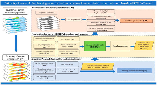
Figure 2.
Estimating framework for obtaining municipal carbon emissions from provincial carbon emissions based on ISTIRPAT model.
4. Results and Discussion
4.1. Model Verification and Comparative Analysis
4.1.1. Verification of ISTIRPAT Model
In this study, the provincial carbon emission panel data were constructed to invert carbon emissions at the municipal level. Although the panel data reduced the non-stationarity of the data and correlations between variables, the variables may still have trend and intercept problems, which may be due to nonstationary data and unit roots. Therefore, in order to avoid false regression when using panel regression, the panel data model must test whether each variable has unit roots before conducting regression analysis. This study mainly adopted the Levin–Lin–Chu (LLC) and ADF–Fisher (ADF) panel root tests [44], and each variable passed the tests (Table 1), indicating no pseudo-regression in the panel data model. Therefore, the intercept term for each factor was obtained in the ISTIRPAT model by a panel data regression of the random effect model (Table 2).

Table 1.
LLC and ADF test results for panel data items (* represents the results under first-order difference).
Table 2.
Regression results for the random effect model of panel data.
The accuracy of the improved carbon emission inversion model was verified. The improved model was used to calculate the carbon emissions in 17 cities and prefectures of Hubei Province over the past seven years, and the data at the county level provided by CEADs were summarized as the true data of carbon emissions at the municipal level. From provincial scale regression and municipal scale calculation and verification, the verification results were obtained at municipal and provincial scales (Figure 3). The accuracy verification showed that the improved model for downscaling from the provincial to municipal level exhibited high accuracy for municipal calculations and better reflected the carbon emissions of cities and prefectures in Hubei Province at the municipal level.
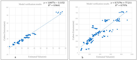
Figure 3.
(a) Verification of municipal scale accuracy in Hubei Province; (b) Verification of provincial scale accuracy in 30 provinces of China.
4.1.2. Comparative Analysis of the Original STIRPAT Model and ISTIRPAT Model
In this study, the carbon emissions for 17 cities and prefectures in Hubei Province estimated by the original STIRPAT and ISTIRPAT models were compared with the real values to verify the accuracy of the improved model. For an intuitive comparison of carbon emissions obtained by the ISTIRPAT model and the original model after downscaling at the municipal scale, a plot representing the city along the -axis, year on the -axis, and carbon emissions on the -axis was generated to evaluate the accuracies of the two models based on the degree of fitting between the surface and the column. As shown in Figure 4, the carbon emissions estimated by the STIRPAT model have a low degree of fit with the real values, especially in areas with high urban carbon emissions, such as Wuhan and Huanggang, and areas with low urban carbon emissions, such as Suizhou, Xiantao, Qianjiang, and other regions, where the estimated values differ substantially from the actual values. The improved STIRPAT model (ISTIRPAT) resolves the issue of low accuracy after downscaling from the provincial level to the municipal level by the construction of urban development factors from nighttime light data. As shown in Figure 4b, the ISTIRPAT model has higher accuracy than that of the original model, including in areas with high or low urban carbon emissions.
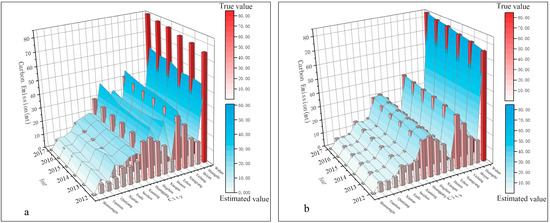
Figure 4.
(a) The fitting effect diagram of original STIRPAT model and real value; (b) The fitting effect diagram of ISTIRPAT model and real value.
To further verify that the ISTIRPAT model has higher accuracy than the original model, the goodness-of-fit for the inversion (estimated) values of carbon emissions at the provincial and municipal scales against the actual values was obtained. Figure 5 compares the degree of fitting between the estimated values obtained by the two models and the actual value at the provincial scale. The value of the ISTIRPAT model at the provincial scale was significantly higher than that of the STIRPAT model. Figure 6 compares the estimation accuracy of the two models at the municipal scale, revealing that the estimation accuracy of the ISTIRPAT model is higher than that of the STIRPAT model.
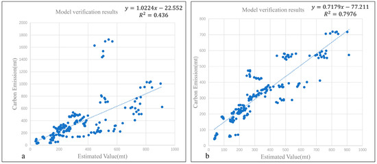
Figure 5.
(a) Verification of municipal scale accuracy in 30 provinces of China by original STIRPAT model; (b) Verification of provincial scale accuracy in 30 provinces of China by ISTIRPAT model.
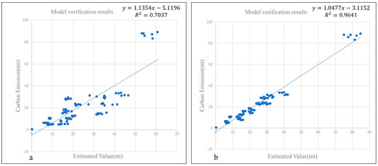
Figure 6.
(a) Verification of municipal scale accuracy in Hubei Province by original STIRPAT model; (b) Verification of provincial scale accuracy in Hubei Province by ISTIRPAT model.
4.2. Analysis of Influencing Factors of Carbon Emissions in Hubei Province
Based on the carbon emissions of the cities and prefectures in Hubei Province from 2012 to 2018 as per the improved STIRAPT carbon emission inversion model, the overall carbon emissions of Hubei Province (Figure 7) increased from 341.035 million tons in 2012 to 398.946 million tons in 2018, with an annual growth rate of 8.273 million tons (Table 3). Cities with large carbon emissions were mainly concentrated in the central region of Hubei Province. Wuhan, Xiangyang, and Yichang cities accounted for the majority of carbon emissions in the province. The total emissions level for the three cities was 142.528 million tons, accounting for 41.79% of the province’s total emissions. The population in the central region is relatively concentrated, and the region has a diverse industrial structure with heavy and manufacturing industries as the main industries; secondary industries accounted for 50% of the GDP. As the city with the highest carbon emissions in Hubei Province, emissions from Wuhan increased from 75.039 million tons in 2012 to 87.153 million tons in 2018. In 2018, Wuhan accounted for 22% of the total carbon emissions of the province, with more rapid growth than other cities. This is mainly due to the large proportion of the total value of secondary industries in the city, such as steel and ships, which mainly consume coal, and the majority of industries consume oil and other fuels which cause more carbon emissions. As the capital city of Hubei Province, Wuhan accounts for 17.5% of the province’s total population, and carbon emissions per capita are expected to be relatively high, resulting in high carbon emissions for Wuhan. The carbon emissions in Shennongjia in western Hubei Province and Tianmen, Qianjiang, and Xiantao in the central region were low in the entire province, ranging from 18.785 million tons in 2012 to 22.045 million tons in 2018, accounting for 5.5% of the total carbon emissions in the province.
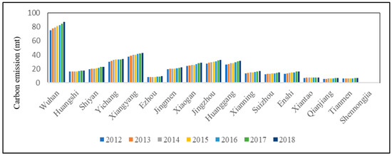
Figure 7.
Carbon emissions from 17 cities and prefectures in Hubei Province, 2012–2018 (million tons).
Table 3.
Estimates of carbon emissions for cities and prefectures in Hubei Province (million tons), 2012–2018, based on the improved model.
Based on carbon emissions per unit of GDP, the process of social development and economic improvement were explored for each city and prefecture in Hubei Province from 2012 to 2018 (Figure 8). The transformation of the industrial structure in various regions and upgrading of technological innovation generally reduced carbon emissions per unit of GDP and reduced energy consumption per unit of GDP. The results show that Wuhan, Xiangyang, and Yichang ranked first in terms of carbon emissions in Hubei Province. However, their carbon emissions per unit GDP were low for the entire Hubei Province. This phenomenon was related to the diversified industrial structures of these cities. As the center of Hubei Province, these cities had relatively complete structures, including primary, secondary, and tertiary industries, and their economic development did not depend entirely on high-carbon emission industries, such as heavy industries. Second, these cities vigorously developed high-tech industries and upgraded steel, shipbuilding, and other industries, effectively reducing energy consumption and promoting rapid economic development. In the western region of Hubei Province, such as Shennongjia and Enshi, carbon emissions and carbon emissions per unit of GDP were both low. This was because the western region of Hubei Province has mountains and the terrain is not flat, making the development of large-scale industrial industries difficult. Therefore, heavy industries and other highly energy-intensive industries associated with high carbon emissions were less common; the main focus was on the development of cultural tourism, catering, and aquaculture, and the industrial structure was biased toward primary and tertiary industries. Based on the dual-carbon target proposed by China, cities and prefectures in Hubei Province need to strengthen the optimization and adjustment of industrial structure to promote the development of service and strategic science and technology industries. Each industry needs to improve energy conversion efficiency to achieve conservation and emission reduction targets through technological upgrading and equipment transformation [45,46]. Regional energy use should focus on the development of low-carbon emissions, such as wind energy, solar energy, and hydropower.
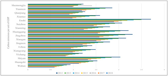
Figure 8.
Carbon emissions per unit GDP in 17 cities and prefectures in Hubei Province, 2012–2018 (10,000 tons/CNY billion).
Using the improved inversion model, the carbon emissions for each city and prefecture were obtained, and the corresponding per capita carbon emissions were calculated (Figure 9). From 2012 to 2018, the per capita carbon emissions of cities and prefectures in Hubei Province increased gradually. Jingmen, Ezhou, Xiangyang, Wuhan City, Wuhan City, and Yichang City in Hubei Province had the highest per capita carbon emissions. Shennongjia, Enshi, Huanggang, and other regions had low carbon emissions per capita. This can be explained by the high per capita GDP of Wuhan, Yichang, Xiangyang, and other regions, which led to greater consumption and greater demand by urban residents in daily life. Therefore, carbon emissions based on terminal consumption were high. As a developing country, increases in urban economic development, urban construction, and per capita GDP in China are necessary to meet national needs and development requirements. Hubei Province, as a development hub in central China, is in the process of urban development; therefore, the consumption level of residents has increased gradually, resulting in inevitable increases in carbon emissions [47,48]. Therefore, for Hubei Province to achieve peak carbon emissions in 2030, cities need to complete the majority of infrastructure construction within 10 years. To reduce carbon emissions from terminal consumption, cities need to strengthen energy management, formulate carbon emission intensity standards with legal requirements for the industry, strengthen low-carbon life propaganda for urban residents, encourage families to use low-carbon lifestyles to save energy, promote low-carbon economic development, and achieve sustainable economic development in the future.
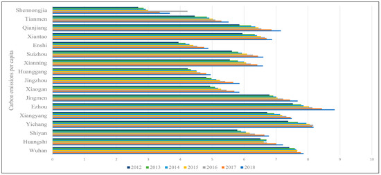
Figure 9.
Per capita carbon emissions from 17 cities and prefectures in Hubei Province, 2012–2018 (tonnes/person).
4.3. Spatial and Temporal Pattern of Carbon Emissions in Hubei Province
We applied the improved STIRPAT carbon emission inversion model (Figure 10) and obtained the standard deviation ellipse of carbon emissions from 2012 to 2018 (Figure 11). According to its location, the overall carbon emissions in Hubei Province are generated from the northwest to the southeast, forming the main carbon emission ring in Hubei Province involving Wuhan, Xiangyang, Yichang, and Jingzhou. Among them, the carbon emissions in Tianmen, Xiantao, and Qianjiang were relatively low in the province. Cities around the ring and adjacent to other provinces account for approximately 28% of the total carbon emissions in Hubei Province.
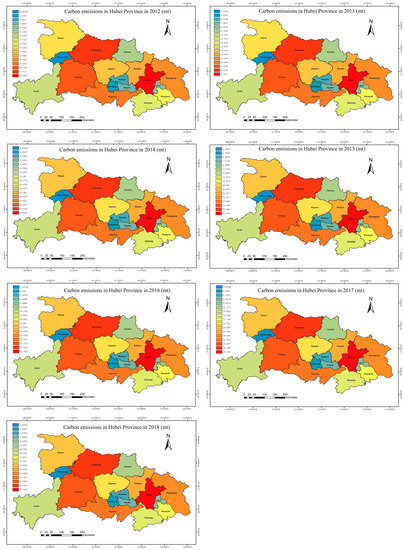
Figure 10.
Carbon emission results for 17 cities and prefectures in Hubei Province from 2012 to 2018.
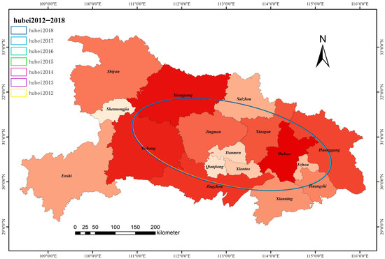
Figure 11.
Standard deviation ellipse for Hubei Province 2012–2018.
From a geographical point of view, most cities and prefectures in western Hubei Province are in mountainous areas, and the population distribution is relatively scattered. Carbon emissions in the region account for 29% of the carbon emissions of the whole province. The cities and prefectures in eastern Hubei rely on the Yangtze River and its tributaries, and the population is concentrated. This region accounts for 41% of the total carbon emissions in the province. Central Hubei is located in the plains; however, its carbon emissions account for only 30% of the total in the province. Hubei Province, as an important center of the Yangtze River Economic Belt, relies on Wuhan, Yichang, Huanggang, and Jingzhou in the Yangtze River Basin. These cities have diversified industrial structures and high levels of urbanization, which have been at a high level of carbon emissions in Hubei Province [49]. From a horizontal perspective, eastern Hubei Province has high carbon emissions, while western Hubei Province has low carbon emissions. Enshi Autonomous Prefecture and Shennongjia are the main cities in western Hubei Province. Their urban functions are mainly tourism and agriculture. The overall vegetation coverage in the city is high, and the industrial sector is small, resulting in less overall carbon emissions in the city.
Hubei Province proposed to build the ‘8 + 1’ urban circle by utilizing the geographical position of Wuhan in the Yangtze River Economic Belt and surrounding cities. The city circle covers Huangshi, Ezhou, Huanggang, Xiaogan, Xianning, Xiantao, Tianmen, Qianjiang, and eight cities, including industry, transportation, and other fields, and its economic development is the highest among areas in Hubei Province. Yichang City and Xiangyang City form the Yijing Jing Urban Agglomeration and Xiangshi Sui Urban Agglomeration. Based on the Yangtze River Basin, Xiangyang, Shiyan, and Suizhou are the three main cities in the urban agglomeration of Xiangyang, Shiyan, and Suizhou. They are adjacent to each other and are located in the northern Hubei automobile industry corridor. The automobile industry is also the main economic pillar of the urban agglomeration. In the process of development, the automobile industry contributes substantially to the high carbon emissions of Xiangyang City, the core city of the urban agglomeration, ranking second in Hubei Province. However, the Yijing-Jingjing urban agglomeration is mainly located in the central and southwest areas of Hubei Province and is composed of three prefecture-level cities, Yichang, Jingzhou, and Jingmen. It has abundant products and is located in the chemical industry corridor of Hubei Province. The chemical industry plays a leading role in the urban economy. These industries have an important impact on the city’s carbon emissions, accounting for 24.7% of the carbon emissions in the province.
5. Conclusions
In this paper, the urban development factor (CDE) based on nighttime light remote-sensing data as well as the improved STIRPAT model (ISTIRPAT) was proposed. Incorporating nighttime light data, the improved STIRPAT carbon emission inversion model (ISTIRAPT) accurately estimates the carbon emissions from provincial-level downscaling to the municipal level. Taking Hubei Province as an example, the carbon emissions of 17 cities and prefectures in Hubei Province from 2012 to 2018 were calculated, and the spatial and temporal patterns of carbon emissions in Hubei Province were analyzed. The following conclusions were drawn.
- (1)
- The improved STIRPAT carbon emission inversion model has a carbon emission inversion accuracy of 0.96 at the municipal level, accurately reflecting the carbon emissions of 17 cities and prefectures in Hubei Province from 2012 to 2018. This verifies that the carbon emission inversion model proposed in this paper has high inversion accuracy and a high degree of model fitting.
- (2)
- Since 2012, the carbon emissions in Hubei Province have increased steadily, forming a circular pattern radiating from Wuhan, Xiangyang, Yichang, and Jingzhou as the main carbon-emitting cities, with low carbon emissions in the central region of Hubei Province and high carbon emissions in the marginal cities. The formation of this pattern was related to the distribution of the residential population and regional industrial structure in Hubei Province.
- (3)
- From 2012 to 2018, carbon emissions increased in cities and prefectures in Hubei Province, and the annual growth rate in the province was highest in Wuhan. Despite the increase in overall carbon emissions, the carbon emissions per unit of GDP for 17 cities in Hubei Province show a downward trend. This trend reflects the positive effects of the adjustment of industrial structure and technological upgrades in the whole province. As a result, many carbon emission enterprises are gradually improving their energy efficiency, resulting in improved economic gains while reducing environmental pollution.
The improved STIRPAT carbon emission inversion model proposed in this paper can be applied to calculate carbon emissions in other provinces and regions. It showed a high inversion accuracy at the municipal level. With the spread of COVID-19 worldwide, human activities have been significantly reduced, and the impact of the epidemic needs to be considered in future carbon emission estimations and predictions [50,51]. In future research, we will apply system dynamics, GM gray prediction models, and multi-source remote-sensing data [52,53,54] to simulate and predict future social development scenarios. This will provide a basis for more effective decision making and recommendations to balance the relationship between economic restructuring and dual carbon goals.
Author Contributions
Conceptualization, Q.W. and J.H.; methodology, Q.W.; software, Q.W.; validation, H.Z. and J.H.; formal analysis, J.S.; investigation, M.Y.; resources, Q.W.; data curation, Q.W.; writing—original draft preparation, Q.W.; writing—review and editing, J.H.; visualization, Q.W.; supervision, J.H. All authors have read and agreed to the published version of the manuscript.
Funding
This research was funded by the National Natural Science Foundation of China, grant number 42001018, 41071104.
Institutional Review Board Statement
The study did not require ethical approval.
Informed Consent Statement
Informed consent was obtained from all subjects involved in the study.
Conflicts of Interest
The authors declare no conflict of interest.
References
- Liu, N.; Ma, Z.; Kang, J. Changes in carbon intensity in China’s industrial sector: Decomposition and attribution analysis. Energy Policy 2015, 87, 28–38. [Google Scholar] [CrossRef]
- Akram, Z.; Engo, J.; Akram, U.; Zafar, M.W. Identification and analysis of driving factors of CO2 emissions from economic growth in Pakistan. Environ. Sci. Pollut. Res. 2019, 26, 19481–19489. [Google Scholar] [CrossRef] [PubMed]
- Yasmeen, H.; Wang, Y.; Zameer, H.; Solangi, Y.A. Decomposing factors affecting CO2 emissions in Pakistan: Insights from LMDI decomposition approach. Environ. Sci. Pollut. Res. Int. 2019, 27, 3113–3123. [Google Scholar] [CrossRef] [PubMed]
- Tang, D.; Ma, T.; Li, Z.; Tang, J. Trend Prediction and Decomposed Driving Factors of Carbon Emissions in Jiangsu Province during 2015–2020. Sustainability 2016, 8, 1018. [Google Scholar] [CrossRef]
- Chen, J.; Wu, Y.; Song, M.; Dong, Y. The residential coal consumption: Disparity in urban–rural China. Resour. Conserv. Recycl. 2018, 130, 60–69. [Google Scholar] [CrossRef]
- Wen, L.; Shao, H. Analysis of influencing factors of the carbon dioxide emissions in China’s commercial department based on the STIRPAT model and ridge regression. Environ. Sci. Pollut. Res. 2019, 26, 27138–27147. [Google Scholar] [CrossRef]
- Lohwasser, J.; Schaffer, A.; Brieden, A. The role of demographic and economic drivers on the environment in traditional and standardized STIRPAT analysis. Ecol. Econ. 2020, 178, 106811. [Google Scholar] [CrossRef]
- Zhang, P.; He, J.; Hong, X.; Zhang, W.; Qin, C.; Pang, B.; Li, Y.; Liu, Y. Regional-Level Carbon Emissions Modelling and Scenario Analysis: A STIRPAT Case Study in Henan Province, China. Sustainability 2017, 9, 2342. [Google Scholar] [CrossRef]
- Liu, D.; Xiao, B. Can China achieve its carbon emission peaking? A scenario analysis based on STIRPAT and system dynamics model. Ecol. Indic. 2018, 93, 647–657. [Google Scholar] [CrossRef]
- Noorpoor, A.R.; Kudahi, S.N. CO2 emissions from Iran’s power sector and analysis of the influencing factors using the stochastic impacts by regression on population, affluence and technology (STIRPAT) model. Carbon Manag. 2015, 6, 101–116. [Google Scholar] [CrossRef]
- Yuan, R.; Zhao, T.; Xu, X.S.; Kang, J.D. Regional Characteristics of Impact Factors for Energy-Related CO2 Emissions in China, 1997–2010: Evidence from Tests for Threshold Effects Based on the STIRPAT Model. Environ. Modeling Assess. 2015, 20, 129–144. [Google Scholar] [CrossRef]
- Zuo, Z.; Guo, H.; Cheng, J. An LSTM-STRIPAT model analysis of China’s 2030 CO2 emissions peak. Carbon Manag. 2020, 11, 577–592. [Google Scholar] [CrossRef]
- Xu, G.Y.; Wang, W.M. China’s energy consumption in construction and building sectors: An outlook to 2100. Energy 2020, 195, 117045. [Google Scholar] [CrossRef]
- Font Vivanco, D.; Kemp, R.; van der Voet, E.; Heijungs, R. Using LCA-based Decomposition Analysis to Study the Multidimensional Contribution of Technological Innovation to Environmental Pressures. J. Ind. Ecol. 2014, 18, 380–392. [Google Scholar] [CrossRef]
- Tursun, H.; Li, Z.; Liu, R.; Li, Y.; Wang, X. Contribution weight of engineering technology on pollutant emission reduction based on IPAT and LMDI methods. Clean Technol. Environ. Policy 2015, 17, 225–235. [Google Scholar] [CrossRef]
- Song, M.; Wang, S.; Yu, H.; Yang, L.; Wu, J. To reduce energy consumption and to maintain rapid economic growth: Analysis of the condition in China based on expended IPAT model. Renew. Sustain. Energy Rev. 2011, 15, 5129–5134. [Google Scholar] [CrossRef]
- Zaman, K.; Moemen, M.A. Energy consumption, carbon dioxide emissions and economic development: Evaluating alternative and plausible environmental hypothesis for sustainable growth. Renew. Sustain. Energy Rev. 2017, 74, 1119–1130. [Google Scholar] [CrossRef]
- Wu, C.B.; Huang, G.H.; Xin, B.G.; Chen, J.K. Scenario analysis of carbon emissions’ anti-driving effect on Qingdao’s energy structure adjustment with an optimization model, Part I: Carbon emissions peak value prediction. J. Clean. Prod. 2018, 172, 466–474. [Google Scholar] [CrossRef]
- Di, W.; Rui, N.; Hai-ying, S. Scenario Analysis of China’s Primary Energy Demand and CO2 Emissions Based on IPAT Model. Energy Procedia 2011, 5, 365–369. [Google Scholar] [CrossRef][Green Version]
- Mi, Z.; Zhang, Y.; Guan, D.; Shan, Y.; Liu, Z.; Cong, R.; Yuan, X.-C.; Wei, Y.-M. Consumption-based emission accounting for Chinese cities. Appl. Energy 2016, 184, 1073–1081. [Google Scholar] [CrossRef]
- Dhakal, S. Urban energy use and carbon emissions from cities in China and policy implications. Energy Policy 2009, 37, 4208–4219. [Google Scholar] [CrossRef]
- Shigeto, S.; Yamagata, Y.; Ii, R.; Hidaka, M.; Horio, M. An easily traceable scenario for 80% CO2 emission reduction in Japan through the final consumption-based CO2 emission approach: A case study of Kyoto-city. Appl. Energy 2012, 90, 201–205. [Google Scholar] [CrossRef]
- Caro, D.; Rugani, B.; Pulselli, F.M.; Benetto, E. Implications of a consumer-based perspective for the estimation of GHG emissions. The illustrative case of Luxembourg. Sci. Total Environ. 2015, 508, 67–75. [Google Scholar] [CrossRef] [PubMed]
- Davis, S.J.; Caldeira, K. Consumption-based accounting of CO2 emissions. Proc. Natl. Acad. Sci. USA 2010, 107, 5687–5692. [Google Scholar] [CrossRef]
- Hillman, T.; Ramaswami, A. Greenhouse Gas Emission Footprints and Energy Use Benchmarks for Eight U.S. Cities. Environ. Sci. Technol. 2010, 44, 1902–1910. [Google Scholar] [CrossRef]
- Liu, Y.; Tan, X.-J.; Yu, Y.; Qi, S.-Z. Assessment of impacts of Hubei Pilot emission trading schemes in China—A CGE-analysis using TermCO2 model. Appl. Energy 2017, 189, 762–769. [Google Scholar] [CrossRef]
- Guan, Y.; Kang, L.; Shao, C.; Wang, P. Measuring county-level heterogeneity of CO2 emissions attributed to energy consumption: A case study in Ningxia Hui Autonomous Region, China. J. Clean. Prod. 2017, 142, 3471–3481. [Google Scholar] [CrossRef]
- Zhou, Y.; Chen, M.; Tang, Z.; Mei, Z. Urbanization, land use change, and carbon emissions: Quantitative assessments for city-level carbon emissions in Beijing-Tianjin-Hebei region. Sustain. Cities Soc. 2021, 66, 102701. [Google Scholar] [CrossRef]
- Jing, Q.; Bai, H.; Luo, W.; Cai, B.; Xu, H. A top-bottom method for city-scale energy-related CO2 emissions estimation: A case study of 41 Chinese cities. J. Clean. Prod. 2018, 202, 444–455. [Google Scholar] [CrossRef]
- Propastin, P.; Kappas, M. Assessing Satellite-Observed Nighttime Lights for Monitoring Socioeconomic Parameters in the Republic of Kazakhstan. GIScience Remote Sens. 2012, 49, 538–557. [Google Scholar] [CrossRef]
- Castells-Quintana, D.; Dienesch, E.; Krause, M. Air pollution in an urban world: A global view on density, cities and emissions. Ecol. Econ. 2021, 189, 107153. [Google Scholar] [CrossRef]
- Ghosh, T.; Elvidge, C.D.; Sutton, P.C.; Baugh, K.E.; Ziskin, D.; Tuttle, B.T. Creating a Global Grid of Distributed Fossil Fuel CO2 Emissions from Nighttime Satellite Imagery. Energies 2010, 3, 1895–1913. [Google Scholar] [CrossRef]
- Chen, J.; Gao, M.; Cheng, S.; Hou, W.; Song, M.; Liu, X.; Liu, Y.; Shan, Y. County-level CO2 emissions and sequestration in China during 1997–2017. Sci. Data 2020, 7, 391. [Google Scholar] [CrossRef]
- Sun, Y.; Zheng, S.; Wu, Y.; Schlink, U.; Singh, R.P. Spatiotemporal Variations of City-Level Carbon Emissions in China during 2000–2017 Using Nighttime Light Data. Remote Sens. 2020, 12, 2916. [Google Scholar] [CrossRef]
- Xie, Y.; Weng, Q. World energy consumption pattern as revealed by DMSP-OLS nighttime light imagery. GIScience Remote Sens. 2016, 53, 265–282. [Google Scholar] [CrossRef]
- Cao, X.; Wang, J.; Chen, J.; Shi, F. Spatialization of electricity consumption of China using saturation-corrected DMSP-OLS data. Int. J. Appl. Earth Obs. Geoinf. 2014, 28, 193–200. [Google Scholar] [CrossRef]
- Political Bureau of the Central Committee of the CPC. Outline of Yangtze River Economic Belt Development Plan; Political Bureau of the Central Committee of the CPC: Beijing, China, 2016. [Google Scholar]
- Li, J.; Luo, R.; Yang, Q.; Yang, H. Inventory of CO2 emissions driven by energy consumption in Hubei Province: A time-series energy input-output analysis. Front. Earth Sci. 2016, 10, 717–730. [Google Scholar] [CrossRef]
- Dietz, T.; Rosa, E.A. Effects of population and affluence on CO2 emissions. Proc. Natl. Acad. Sci. USA 1997, 94, 175–179. [Google Scholar] [CrossRef]
- Kuznets, S. Economic Growth and Income Equality. Am. Econ. Rev. 1955, 45, 1–28. [Google Scholar]
- Grossman, G.; Krueger, A. Environmental Impacts of the North American Free Trade Agreement. Q. J. Econ. 1995, 110, 3914. [Google Scholar]
- Qiang, Y.; Huang, Q.; Xu, J. Observing community resilience from space: Using nighttime lights to model economic disturbance and recovery pattern in natural disaster. Sustain. Cities Soc. 2020, 57, 102115. [Google Scholar] [CrossRef]
- Chen, J.; Wei, H.; Li, N.; Chen, S.; Qu, W.; Zhang, Y. Exploring the Spatial-Temporal Dynamics of the Yangtze River Delta Urban Agglomeration Based on Night-Time Light Remote Sensing Technology. IEEE J. Sel. Top. Appl. Earth Obs. Remote Sens. 2020, 13, 5369–5383. [Google Scholar] [CrossRef]
- Levin, A.; Lin, C.; James Chu, C. Unit root tests in panel data: Asymptotic and finite-sample properties. J. Econom. 2002, 108, 1–24. [Google Scholar] [CrossRef]
- Wang, Q.; Yang, X. Imbalance of carbon embodied in South-South trade: Evidence from China-India trade. Sci. Total Environ. 2020, 707, 134473. [Google Scholar] [CrossRef]
- Yang, L.; Xia, H.; Zhang, X.; Yuan, S. What matters for carbon emissions in regional sectors? A China study of extended STIRPAT model. J. Clean. Prod. 2018, 180, 595–602. [Google Scholar] [CrossRef]
- Dong, F.; Long, R.; Chen, H.; Li, X.; Yang, Q. Factors affecting regional per-capita carbon emissions in China based on an LMDI factor decomposition model. PLoS ONE 2013, 8, e80888. [Google Scholar]
- Li, R.; Wang, Q.; Liu, Y.; Jiang, R. Per-capita carbon emissions in 147 countries: The effect of economic, energy, social, and trade structural changes. Sustain. Prod. Consum. 2021, 27, 1149–1164. [Google Scholar] [CrossRef]
- Liddle, B. Demographic Dynamics and Per Capita Environmental Impact: Using Panel Regressions and Household Decompositions to Examine Population and Transport. Popul. Environ. 2004, 26, 23–39. [Google Scholar] [CrossRef]
- Bustamante-Calabria, M.; Sánchez de Miguel, A.; Martín-Ruiz, S.; Ortiz, J.L.; Vílchez, J.M.; Pelegrina, A.; García, A.; Zamorano, J.; Bennie, J.; Gaston, K.J. Effects of the COVID-19 lockdown on urban light emissions: Ground and satellite comparison. Remote Sens. 2021, 13, 258. [Google Scholar] [CrossRef]
- Jechow, A.; Hölker, F. Evidence that reduced air and road traffic decreased artificial night-time skyglow during COVID-19 lockdown in Berlin, Germany. Remote Sens. 2020, 12, 3412. [Google Scholar] [CrossRef]
- Sánchez de Miguel, A.; Kyba, C.C.; Aubé, M.; Zamorano, J.; Cardiel, N.; Tapia, C.; Jon, B.; Gaston, K.J. Colour remote sensing of the impact of artificial light at night (I): The potential of the International Space Station and other DSLR-based platforms. Remote Sens. Environ. 2019, 224, 92–103. [Google Scholar] [CrossRef]
- Román, M.O.; Wang, Z.; Sun, Q.; Kalb, V.; Miller, S.D.; Molthan, A.; Lori, S.; Jordan, B.; Stokes, E.C.; Pandey, B.; et al. NASA’s Black Marble nighttime lights product suite. Remote Sens. Environ. 2018, 210, 113–143. [Google Scholar] [CrossRef]
- Hung, L.W.; Anderson, S.J.; Pipkin, A.; Fristrup, K. Changes in night sky brightness after a countywide LED retrofit. J. Environ. Manag. 2021, 292, 112776. [Google Scholar] [CrossRef]
Publisher’s Note: MDPI stays neutral with regard to jurisdictional claims in published maps and institutional affiliations. |
© 2022 by the authors. Licensee MDPI, Basel, Switzerland. This article is an open access article distributed under the terms and conditions of the Creative Commons Attribution (CC BY) license (https://creativecommons.org/licenses/by/4.0/).