A Data-Driven Method for Identifying Drought-Induced Crack-Prone Levees Based on Decision Trees

Abstract

In this paper, we aim to identify factors affecting susceptibility to drought-induced cracking in levees and use them to build a machine learning model that can identify crack-prone levees on a regional scale. By considering the key relationship between the size of cracks and the moisture content, we observed that low moisture contents act as an important driver in the cracking mechanism. In addition, factors which control the deformation at low moisture content were seen to be important. Factors that affect susceptibility to cracking were proposed. These factors are precipitation, evapotranspiration, soil subsidence, grass color, soil type, peat layer thickness, soil stiffness and levee orientation. Statistics show that the cumulative precipitation deficit is best associated with the occurrence of the cracks (cracks are characterized by higher precipitation deficits). Model tree classification algorithms were used to predict whether a given input of the factors can lead to cracking. The performance of a model predicting long cracks was evaluated with a Matthews correlation coefficient (MCC) of 0.31, while a model predicting cracks in general was evaluated with an MCC of 0.51. Evaluation of the model trees indicated that the peat thickness, the soil stiffness and the orientation of the levee can be used to determine crack-proneness of the levees. To maintain validity and usefulness of the data-driven models, it is important that asset managers of levees also register locations on which no cracks are observed.

1. Introduction

Many countries in the world are prone to flooding, e.g., the Netherlands, where the majority of its area is located below sea level. For this reason, most of the country relies on flood defense strategies which mostly comprise levees and other man-made flood defenses in order to achieve acceptable flood risk frequencies. Climate change-induced sea level rise and increasingly intense precipitation are expected to increase loads on flood defenses [1]. In addition, persistent dry periods caused by an increase in temperature in combination with less precipitation might lead to a decrease in the performance of existing levees [2], and evidence has shown that sustained drought periods are a hazard for levee stability [3]. For example, in the town of Wilnis, a levee breached in 2003, due to excess evaporation during the summer, which caused a weight reduction such that the levee became sufficiently light to initiate a horizontal sliding mechanism driven by the adjacent water course [4]. Another example was seen in 2008, when the Millennium Drought occurred in Australia. Heavy rainfall after a long period of drought caused failure of a riverbank section of a length of 150 m. As well as this direct failure, the integrity of 300 km of levees was threatened [5].

During sustained dry periods, cracks are observed on levees [6]. When crack depths grow, e.g., the crack reaches dimensions in the order of meters, the levee may become at risk of failure due to macrostability due to an intersection of the crack and a potential sliding plane [7]. Horizontal sliding of the levee, macro-instability and subsidence due to drought are depicted in Figure 1A–C, respectively.

Another effect is that the presence of cracks influences infiltration processes in peat and clay soils in the form of preferential flow paths [3,8], leading to changes in pore pressure and a decrease in the effective stresses [9]. Furthermore, in cases of extreme precipitation, cracks may fill with water, exerting additional loads on the levees [9]. Past studies have shown the mechanical behavior of cracks which was induced by dry conditions [10] on the scale of the cracks themselves. As a result of the increase in awareness of drought hazards, levee asset managers in The Netherlands have begun inspecting the levees during dry periods more frequently. The choice for the specific levees which are inspected is usually based on expert judgment. With the frequency of drought events increasing, it is important to predict and detect the occurrence of cracks in clay and peat levees so that components of the flood defense system resilience such as resistance, absorption and adaptation are strengthened. This will also allow the improvement of inspection and monitoring systems which at the moment are conducted based on periodic human visual evaluations.

In this study, we explore the potential of a data-driven approach that allows us to understand not only the drivers of cracking on clay and peat levees, but also their spatial distribution. For infrastructural asset management purposes, machine learning models are currently regularly applied to assess the condition of infrastructure assets. In pavement engineering for example, artificial neural networks and random forests were used for detecting and classifying cracks in pavement structures [11]. Research on dam site suitability [12] has shown that the application of machine learning techniques contributes to a better accuracy in determining suitable sites than the application of present decision-making tools only. For flood defenses, Jamalinia et al. [13] examined the possibility of using earth observation within a random forest framework to identify vulnerable levee locations. Vegetation and deformation were shown to be strongly correlated with the response of a levee to water content and therefore cracking on a hypothetical levee and able to be used in a random forest framework. However, site-specific information needed to be input. Other research has shown [14] that machine learning models can be successful in the prediction of soft soil foundation settlement in levees. The insights gained from the research allow for the application of the data-driven methods to flood defense asset management. The aim of this paper is to leverage the available inspection datasets of levee cracking and to combine them with pre-identified local environmental factors which better correlate to the observations in building a machine learning model that can help to identify crack-prone levees which have not been inspected. The added benefit of this knowledge comes in the form of improved asset management and therefore a lower hazard of drought. The paper is structured as follows: Section 2 outlines the literature study on proposing factors that contribute to the cracking mechanism. Section 3 presents the methodology used to collect data, develop a machine learning (random model tree classification algorithm) method to identify vulnerable levees and to generate hazard maps. In Section 4, we elaborate on a case study used to demonstrate the method. Section 5 then presents the results. Section 6 discusses the results and the conclusions are presented in Section 7.

2. Factors Affecting Susceptibility to Cracking

Periods of drought tend to decrease the phreatic level in a levee due to seepage, increasing the depth of the unsaturated zone at the top of the levee [15]. Shrinkage in the levee typically occurs in two phases in time [6,16]; the first in which only subsidence (vertical deformation) is observed and a second one in which vertical and horizontal (not necessarily equal) deformation takes place [17]. During the first period, horizontal stresses are reduced, but remain below the level where cracking can occur. The second phase is initiated after the occurrence of the first crack. Figure 2 displays both stages, in which $t_0$ represents the matrix dimensions after the subsidence stage, and t after subsidence and isotropic shrinkage. The soil cross sectional area after isotropic shrinkage is V, leaving $V^{*}$ as the cracked cross sectional area.

In general, peaty and clay soils shrink substantially when they are subjected to drying conditions, with peat soils shrinking more. In the unsaturated zone of a soil, drier conditions cause the occurrence of matrix suction [16]. The suction in the matrix pulls the particles closer to one another, decreasing the volume, while increasing the density. Soils tend to show different characteristics during either drying or wetting [18], which can result in nonlinear behaviour and potentially irreversible shrinkage.

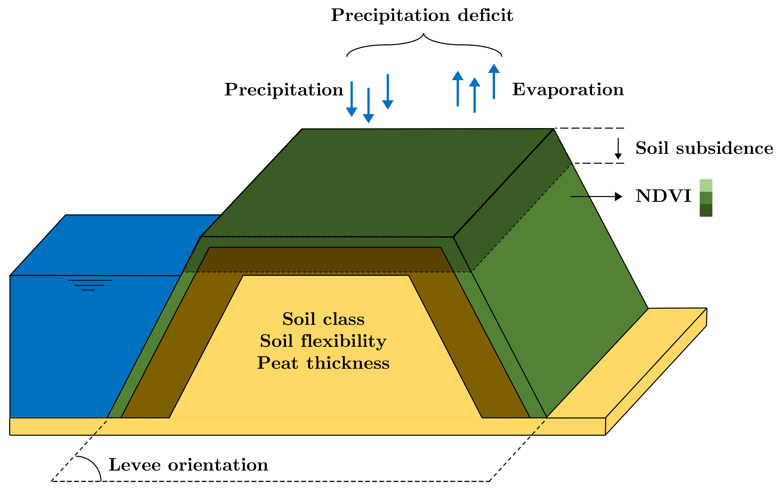
By formulating relationships for both the first and the second phase, Pyatt [17] derived an expression for the fraction of the cracking volume $V^{*}$ with respect to the initial soil volume V. In this expression, the gravimetric soil moisture content at cracking initiation ${\theta }_0$ is a parameter dependent upon the type of soil (peat in that case). Cracking is initiated when the value of gravimetric soil moisture content $\theta$ is lower than ${\theta }_0$. In an ideal situation, we could reach the goal of this paper if ${\theta }_0$ and $\theta$ were constantly known in time and space. This information is, however, not generally available on a detailed scale, and can be dependent on the materials, material state (stress, water content, etc.) and history. Therefore, several factors which influence either ${\theta }_0$ or $\theta$ are considered and reviewed as potential proxies to be used later due to their physical relevance and availability. Figure 3 presents an overview of the considered factors that affect susceptibility to cracking.

2.1. Precipitation Deficit

The definition of drought varies in literature and several indices have been formulated to quantify it [19]. For example, the Dutch meteorological institute KNMI defines drought as a longer period characterized by less precipitation than evaporation. The precipitation deficit is seen as an absolute quantification of this and is considered a key driver for low values of $\theta$. The precipitation deficit is obtained by subtracting the potential evaporation from the precipitation, in which the potential evaporation is estimated according to the method of Makkink [20], taking into account solar radiation and the mean daily temperature [21]. Thanks to weather stations which record frequently, this parameter can be considered at a high temporal resolution, but at a lower spatial resolution (kilometer scale) despite a widespread distribution of weather stations in the Netherlands. The Standardised Precipitation Evapotranspiration Index (SPEI) is an indicator used for the quantification of drought, which is calculated by computing the precipitation deficit and transforming it to the standard normal distribution of precipitation deficit in time. It considers the precipitation deficit for a given period in the year and compares it to the precipitation deficit for the same period over the previous years.

2.2. Soil Subsidence Rate

Vertical shrinkage can be used to indicate whether either of the two phases shown in Figure 2 is occurring (either on or under the levee) and whether the soil is susceptible to shrinkage. Since only soil subsidence is observed in the first shrinking phase (when $\theta$ is decreasing, but still greater than ${\theta }_0$), it may act as an indicator for (future) cracking. In most global locations, high-temporal-fidelity data are not available, therefore, an annual average value is considered to be available here.

2.3. NDVI

Vegetation plays a significant role in the water balance of a soil, and is found on the outer surface of regional levees in the Netherlands in the form of grass. The root zone extracts moisture from the soil in order to complete photosynthesis [22]. As this process produces chlorophyll, the grass gains a more intense green color. A low $\theta$ is therefore represented by a less intense green color. A measure of the color of vegetation is the Normalized Difference Vegetation Index (NDVI), and it can be computed using satellite imagery. It is regularly applied in drought-monitoring studies [23]. The NDVI is computed as:

$$\mathrm{NDVI}=\frac{\mathrm{NIR}-\mathrm{Red}}{\mathrm{NIR}+\mathrm{Red}}$$

(1)

where NIR represents the spectral reflectance measurement of the near-infrared spectrum, and Red—the reflection in the (visible) red range of the visible light spectrum. There can be a time delay expected between a low $\theta$ and the NDVI values.

2.4. Soil Class/Type

Different soil types are associated with different soil behavior, including the shrinkage behavior [24] and, therefore, cracking. The upper layers immediately below a levee can partially control the water drainage and deformation and, therefore, can be considered as a potential proxy. The considered proxy is defined as a nominal variable.

2.5. Peat Layer Thickness

The thickness of shrinkage-susceptible layers in the levee strongly influences the cracking potential. As peat has the highest ability to shrink, the thickness of any peat layer in the upper (unsaturated) part of the soil body is considered.

2.6. Soil Stiffness/Flexibility

The kinematic resistance of a soil matrix to a mechanical load is accounted for as the soil stiffness. It is expected that a high stiffness of the soil is correlated with a low ${\theta }_0$, as the soil does not significantly deform after changes in suction and, therefore, horizontal stresses do not easily become tensile. As the soil column is layered and layer thickness is an important aspect in the deformation, the soil flexibility can be used. The soil flexibility [25] is defined as the irresistance of a soil layer to settlements due to a load (units m/kPa).

2.7. Levee Orientation with Respect to the Sun

The orientation of a levee influences the exposure to solar energy. A levee with a southerly facing sloping face may receive more solar energy, enhancing the evaporation. This has not been accounted for in the precipitation deficit, which has a kilometer-scale spatial resolution. The orientation of the levee is therefore assumed to be an independent driver for cracking.

3. Method

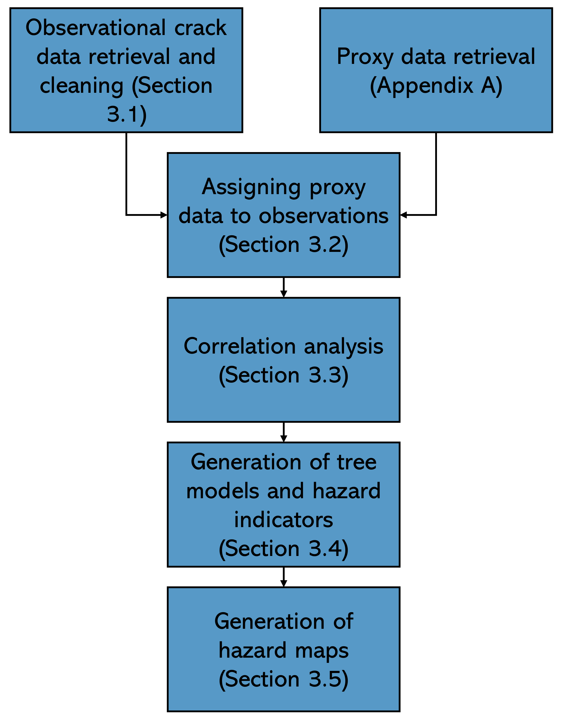
Figure 4 shows a schematic overview of the methodology. Firstly, a database was obtained in which observed cracks from manual levee inspections were included. This database was thereafter extended with the possible proxies presented in Section 2. Correlation studies were then conducted to investigate which of those factors can contribute to a prediction of the occurrence of cracks. Model tree classification algorithms were then used to generate a model to predict whether a crack occurs for a given input of proxy variables. The structure of the model trees was finally extracted and used to define hazard indicators, which act as the foundation of identifying crack-prone levees and visualizing those in hazard maps.

3.1. Observational Data Retrieval on Cracks and Proxies

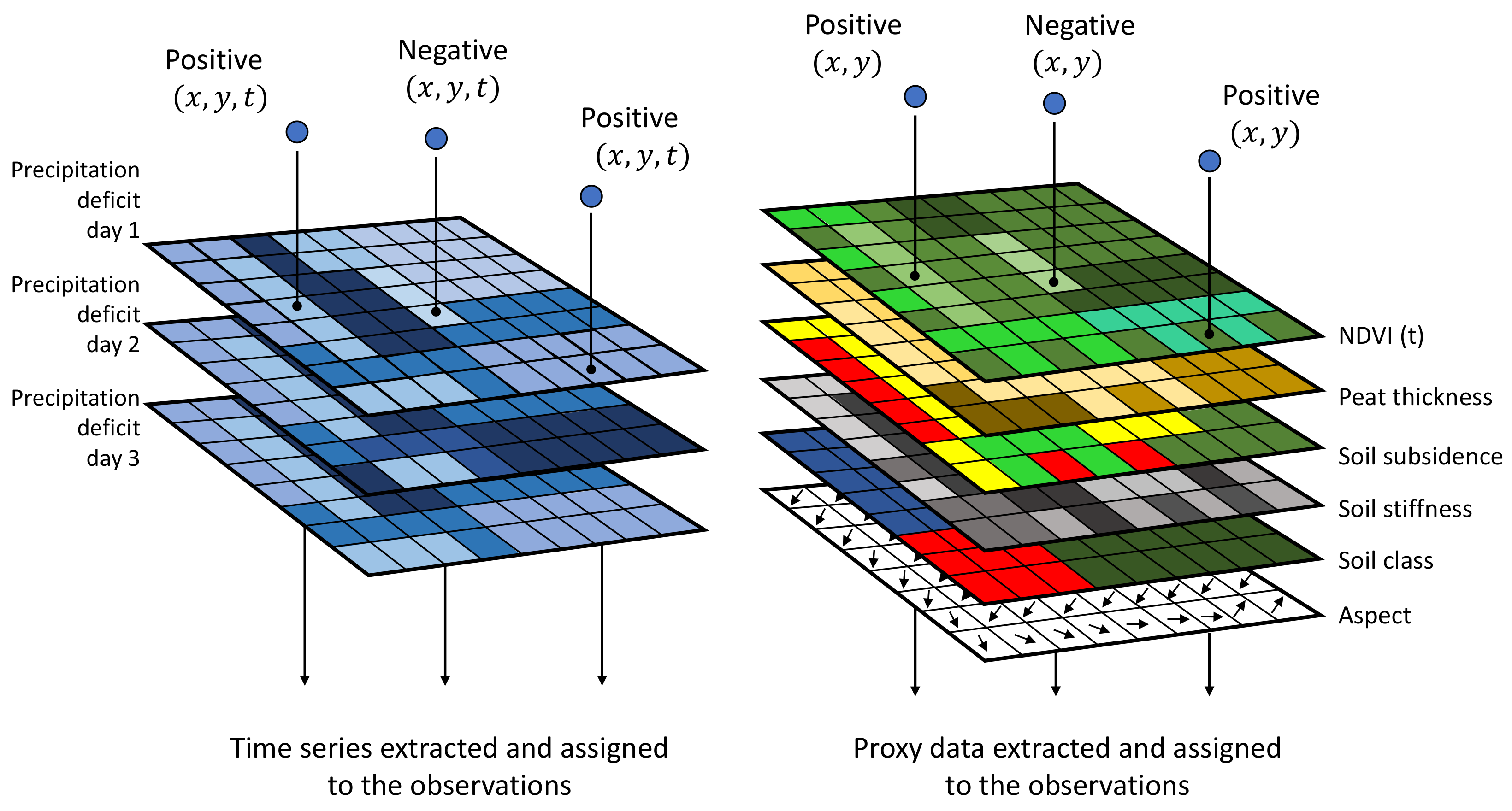
The first step in the construction of the database consisted of the retrieval of observations of drought-induced cracks. The database needs to include the physical locations and time of observed cracks. It is preferred that this database consist of spatiotemporal coordinates on which cracks were registered (positives), as well as coordinates on which no cracks (negatives) were observed. In the case that the amount of positives highly outclasses the negatives (or vice versa), a random sampling method is necessary to balance the database, since the amounts of positives and negatives differ significantly. Since the retrieved database mainly consisted of positives, random negatives were generated. To avoid points that have nearly identical spatiotemporal coordinates, but are registered as both positives and negatives, intervals were constructed enclosing the positives in space and time. The method implies negative samples outside these intervals. After obtaining the database, cleaning it is necessary in order to verify that no (unjust) double registrations are stored. The presence of those might impact the outcome of the classification algorithm as too many positives would lead the algorithm to classify more levees as crack-prone than is realistic. After the retrieval of the observational data on cracks, data related to the proxy variables were retrieved. The proxy data were included in the inspection database by evaluating the data at the spatiotemporal coordinates of the crack observations. For proxies with temporally changing characters, e.g., the precipitation deficit, an observation with coordinates (x, y, t) is needed. For time-independent properties, e.g., the peat thickness, observations only had to be evaluated on spatial coordinates (x, y). Figure 5 depicts the above discussed procedure.

3.2. Correlation Analysis

The individual prediction capacity of the proxies was determined by computing the Cramérs V correlation [26] between the proxies and the state of the observations. By computing the Cramérs V, we facilitate in the association between nominal (categorical variables without order) and ordinal (categorical variables with order) proxies, as well as numerical ones, resulting in a homogeneous comparison between the association of the proxies. Since the precipitation deficit over a period of time may affect the susceptibility of a levee to crack, a time lag correlation analysis was performed. The Cramérs V value was computed for the cumulative precipitation deficit and the state of the observations for lengths of time of a single day prior to the observation until 249 days prior to the observation. The period which had the maximum Cramérs V value was selected as the proxy and assigned to the database.

3.3. Generation of Tree Models

A model tree classification algorithm [27] was used in order to train models. A decision tree model was applied in order to allow for an investigation of the input proxies and binary value of cracking or not. Model trees make predictions by evaluating a given dataset and defining decision rules that split the dataset, creating new subdatasets (nodes). The algorithm attempts to define the decision rules such that the resulting nodes contain as much of one prediction variable (in this case positives/negatives) as possible, in which a node containing only positives is called a pure node. The Gini impurity [27] measures the impurity of a node, where a pure node is evaluated with a Gini impurity of 0, while an (utmost) impure node is evaluated with a Gini impurity of 0.5. The Gini impurity is defined as a measure of how often a randomly chosen element from a set would be incorrectly labeled if it were randomly labeled according to the distribution of labels in the subset [28]. The algorithm keeps splitting the nodes until no further decrease in Gini impurity can be gained (see Figure 6 for a graphical representation). New predictions are made by following the decision rules and classifying the prediction variable as the variable that makes up the majority of the resulting node. A part of a given dataset can be used to construct the decision tree (training set), whereas the remaining dataset can be used to evaluate the performance of the decision tree (test set).

The model was trained to predict the state of an observation, given evidence in the form of the proxy variables. Feature importances [29] were calculated to express the weight of the proxies when the observation state had been predicted. Proxies of which the feature importance was equal to (nearly) 0 can be removed from the database. The performance of the models was thereafter quantified by computing the model accuracies [29] and the Matthews correlation coefficient (MCC), which is defined as [30]:

$$\mathrm{MCC}=\frac{TP·TN-FP·FN}{\sqrt{(TP+FN)(TP+FP)(TN+FP)(TN+FN)}}$$

(2)

in which $TP$, $TN$, $FP$ and $FN$ are defined as true positives, true negatives, false positives and false negatives, respectively. The MCC was further investigated by constructing confusion matrices [29]. The confusion matrices show the amount of $TP$, $TN$, $FP$ and $FN$ in each cell of the matrix. By constructing this matrix, one easily observes to what extents the models correctly predict either positives or negatives (or both). An iterative process was used in order to construct decision trees with a limited depth (defined as pruning) to avoid overfitting of the data and safeguard interpretation. Iteration is necessary for the convergence to a balance between the generalization of the model and preferred performance. Easily in time predictable proxies which distinguish positives and negatives in the model trees were extracted and the criteria resulting in positives were defined as hazard indicators. In this work, this means that all deterministic proxies directed to positives were defined as hazard indicators. For insight in the performance metric, MCC values close to 0 indicate that the model guesses randomly [31], given the interval [−1, 1] and values near 0.5 are good indicators.

3.4. Generation of Hazard Maps

In order to generate spatial insight into crack-prone levees, random points have been sampled in space throughout the area of concern (see Section 4) on levee locations. Each point was assigned the values of the hazard indicator corresponding to that coordinate (for example, the NDVI at that location, if it were a hazard indicator that can distinguish between positive and negatives). Points for which data were assigned that do not meet the hazard indicators were eliminated from the database. This resulted in points in space representing locations of which the data meet the hazard indicators criteria. These remaining points were then projected perpendicularly onto the levees, after which they were split up into sections of 100 m. By counting the number of sampled points projected upon the levee sections, the crack-proneness of the sections was quantified. For comparison, an empirical hazard map was created, in which the observed cracks over the years were projected onto the same levee segments.

4. Case Study

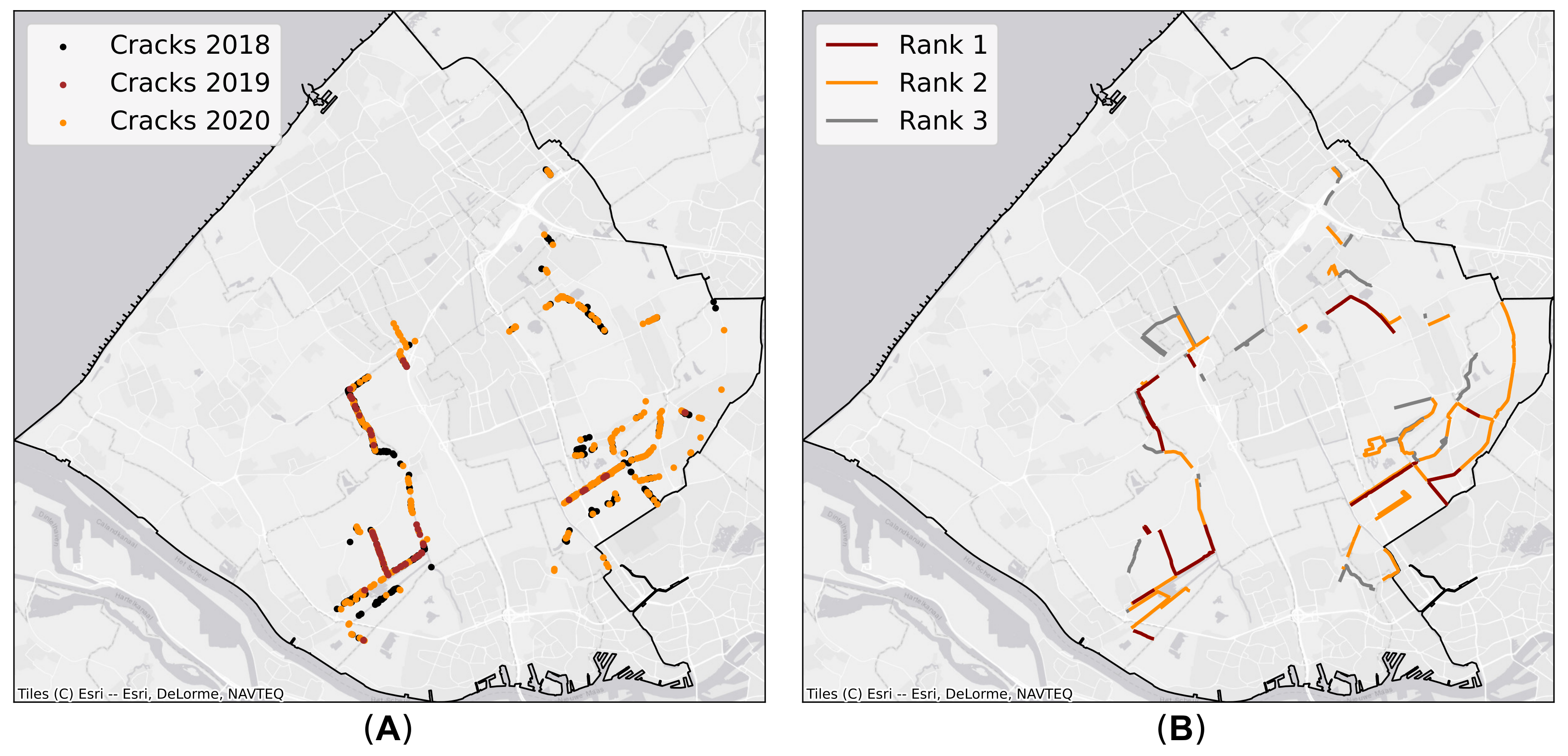
A database was obtained which consisted of observations of cracking from the waterboard Hoogheemraadschap Delfland (HHD) during the years 2018, 2019 and 2020. Information from previous years was also obtained, however, this was not used due to data inconsistencies, such as missing spatial coordinates. HHD is responsible for the asset management of primary and secondary levees within a part of the province of South Holland in the Netherlands. The inspectors increase the inspection frequency between April and September (their fixed definition of the dry season) to gain an improved insight in the location of the cracks in the levees. Figure 7A shows a plot of the area HHD is responsible for (outlined in black), along with the observed cracks during the different years. In the past, HHD performed an expert judgment analysis for the purpose of understanding the spatial crack-proneness of the levees. The analysis resulted in a selection of levees which all were subdivided in three different drought-proneness ranks. The geographical configuration of the ranks is displayed in Figure 7B.

The levees belonging to Rank 1 are inspected during the dry season when the SPEI [32] value calculated for the KNMI station at Rotterdam is lower than −1. Levees belonging to both Rank 1 and 2 are inspected when the SPEI values are lower than −1.75. All ranked levees are inspected when a SPEI value lower than −2.25 is observed.

4.1. Inspection Database

Every two weeks, HHD evaluated the SPEI value to decide upon the levees which were inspected. The inspectors walk along the selected levees and register all observed anomalies, which involve the occurrence of cracks and several observations other than cracks as well (large local subsidence, for example). When the observed anomaly concerns a crack, the dimensions and the location of the crack on which specific part of the levee were usually registered, as well. Finally, the direction of the crack with respect to the orientation of the levee on which it is situated was recorded. Due to inconsistencies in this part of the database, these last 3 aspects were not defined as prediction targets in this case study, however with improved data collection, these could be included within this methodology.

4.2. Generation of Negative Observations

The inspection procedure of HHD results in a database which only contains registrations of positives, as negatives were not registered. Since classification methods are used to predict the occurrence of drought-induced cracks, it was necessary that locations in space and time of negatives had to be acquired as well. To obtain these, two different models were constructed, for which the negatives were generated differently. For Model 1, the negatives were generated by defining all cracks with a length of less than 2 m as a negative. This also facilitates reducing the amount of false negatives within the database, as it might occur that inspectors miss cracks with small dimensions during the visual inspections. Larger cracks also tend to more significantly negatively influence the structural integrity of levees [3], making it more interesting to be able to predict them. To obtain the negatives for Model 2, a sampling technique was used, which considered the spatiotemporal coordinates of positives and sampled negatives at a significant distance of the positives both in space and time. As the number of negatives was significantly greater than the number of positives in Model 2, an oversampling technique [33] was used to decrease the difference in the number of positives and negatives.

4.3. Database with Proxies

Table 1. All the proxies which were accounted for in the study.

Proxy	Definition
Precipitation deficit	Cumulative precipitation deficit over computed period
Aspect	Anticlockwise angle of the levee with respect to the west
Soil flexibility	Deformation of the soil when loaded mechanically
Soil class	Nature and constitution of topsoil
Peat thickness	Thickness of the upper peat layer of a levee
Soil subsidence	Average annual subsidence between 2015 and 2019
NDVI	Difference between near-infrared and red light

displays an overview of all information corresponding to one observation in the database, after the proxies were assigned to the inspection database. Since the locations and date of observations were only used for assigning the proxy variables, the information was dismissed from the database. Table 1 shows all information used in the classification model tree algorithms. For a complete elaboration on the retrieval and the technicalities, the reader is referred to Appendix A.

5. Results

5.1. Time Lag Correlation Analysis of the Precipitation Deficit

Figure 8 shows the lagged correlation results for the period against the state of the observations (crack observed or not). The peaks of the correlations are marked with a red dot.

Both curves show a similar form. Model 1 is characterized by lower Cramérs V values than Model 2. Both models feature an initial peak after approximately 4 days, followed by a sharp decrease until approximately 20 days, and then a slow increase and plateau to 200 days, followed by a rapid decrease. The global peaks of the curves, however, are found on different locations, with Model 1 peaking at the first local peak and Model 2 peaking in the second local peak. This implies that different periods of cumulative precipitation history should be used depending on the classification target. The maximum correlations are found at a period of 4 days and 123 days for Model 1 and Model 2, respectively. The corresponding correlation values are equal to 0.44 and 0.65, respectively.

5.2. Correlation Matrix

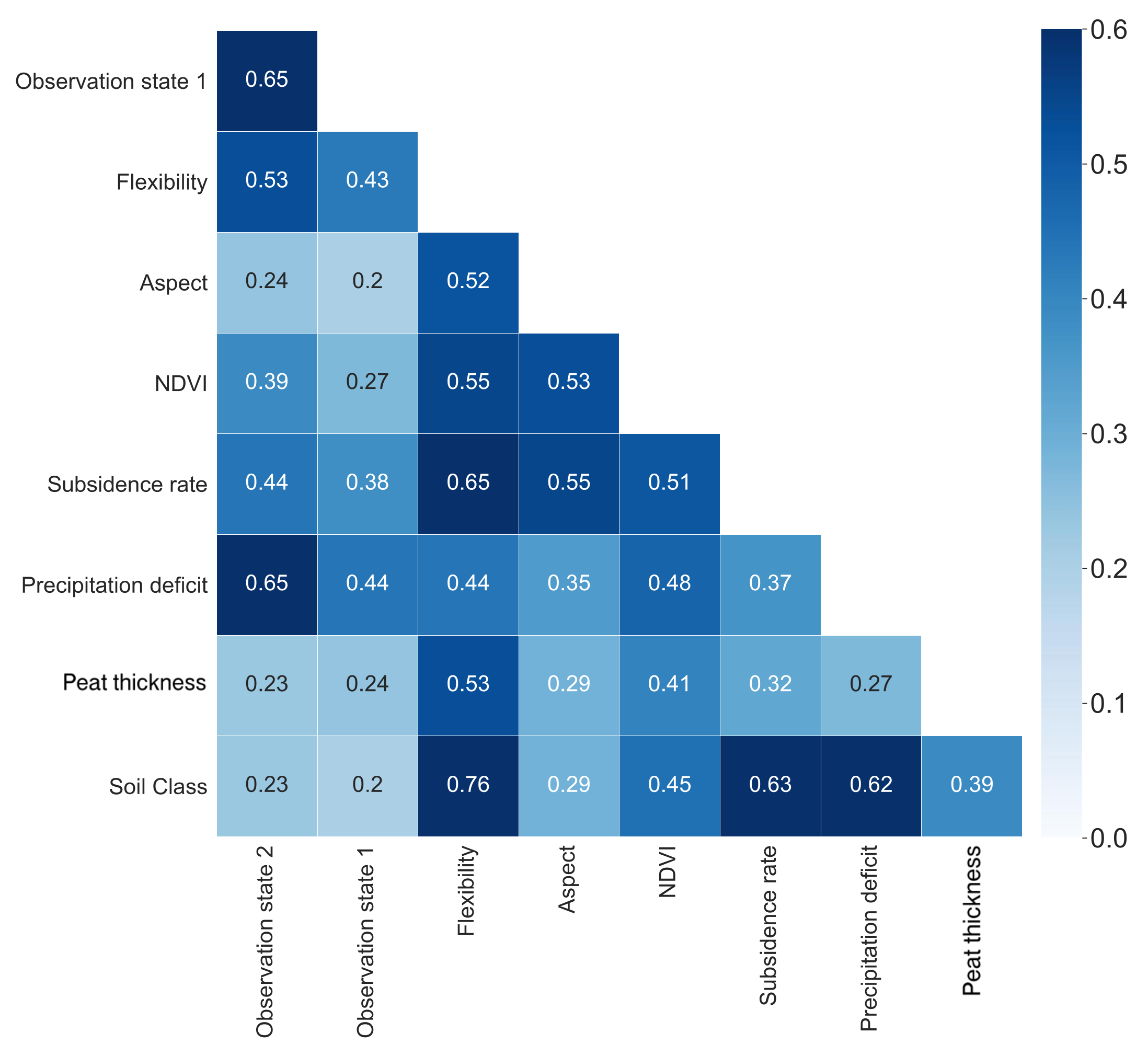
Figure 9 shows an overview of the correlation matrix among the proxies. Note that the soil stiffness is represented by “Flexibility”.

The correlations indicate that the cumulative precipitation deficit is best correlated with the state of the observation of Model 2 (defined as Observation state 2), quantified by a Cramérs V of 0.65 (as seen in Figure 8). Note that a Cramérs V value of 0.65 is not extortionately high, while it is a relatively high value among the data set. This implies that the considered proxies are not that extortionately great at distinguishing between positives and negatives by themselves, whereas the precipitation deficit is best at this. It is also observed that the peat thickness performs worst at distinguishing the positives and negatives. By itself, the peat thickness therefore has the lowest predictive capacity, together with the aspect.

It must be stated however, that the Cramérs V values only indicate the association between the proxies and the observation state themselves. The association between multiple proxies and the observation state should be modeled with a different statistic measure. In this research, this was achieved by evaluating the performance of the model trees as a whole.

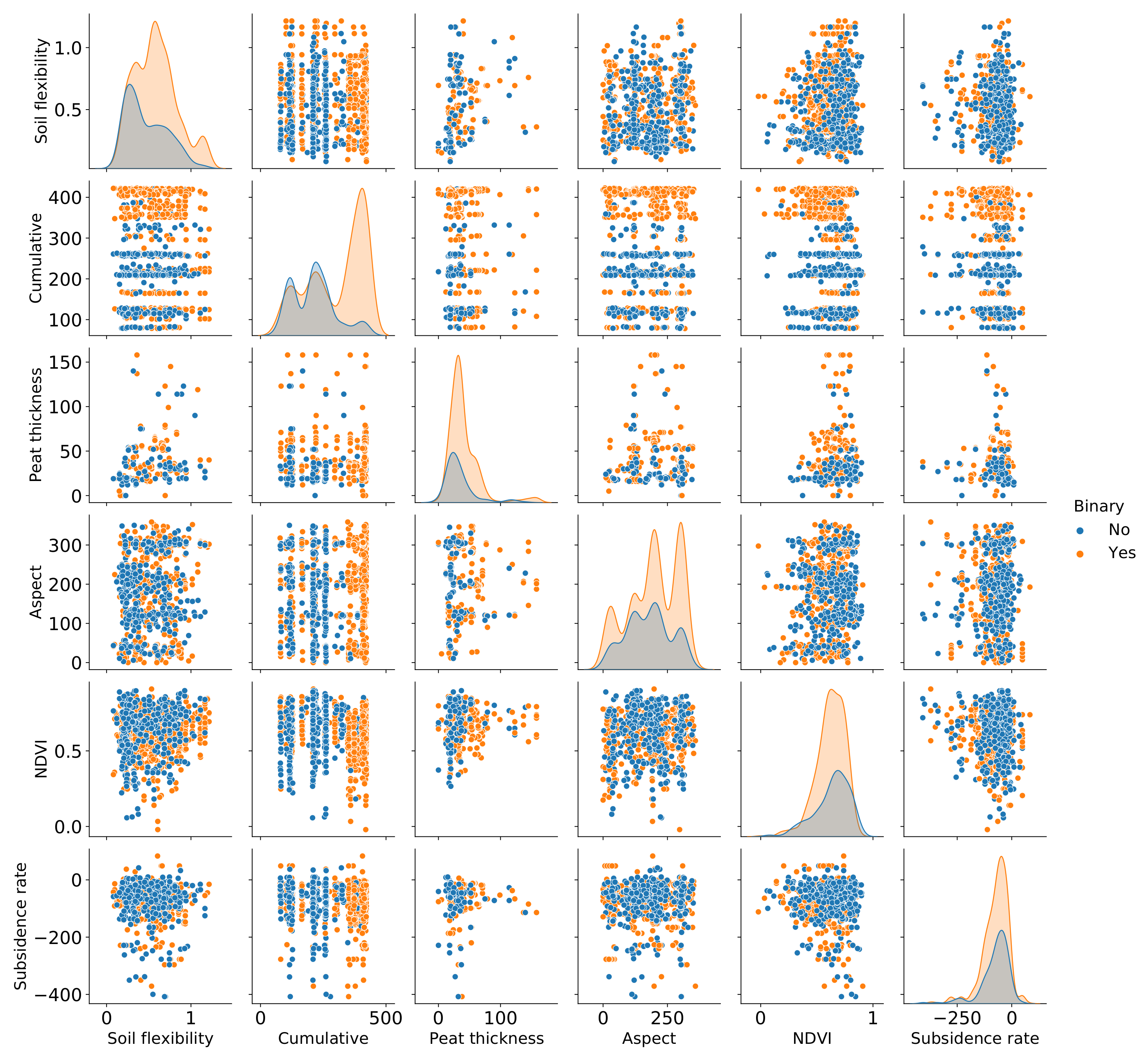
Figure 10 demonstrates scatter plots of all the proxy variables which are represented by numerical variables (categorical variables cannot be plotted on numerical axes). Scatter plots for all possible pairs of proxy variables were plotted, and the color of the points represents the positives (orange) and negatives (blue). In the diagonals, the data of the proxy variables are visualized by constructing histograms and again separating positives from negatives. For the sake of clarity, only the scatter plots for Model 1 are presented.

Here, it can be seen that the precipitation deficit shows a distinction between the positives and the negatives. When the proxy is plotted against the various other ones, the positives are most of the time characterized by a high precipitation deficit. This distinction confirms the observation seen in Figure 9, stating that the precipitation deficit is evaluated with the highest Cramérs V correlation against the state of the observations.

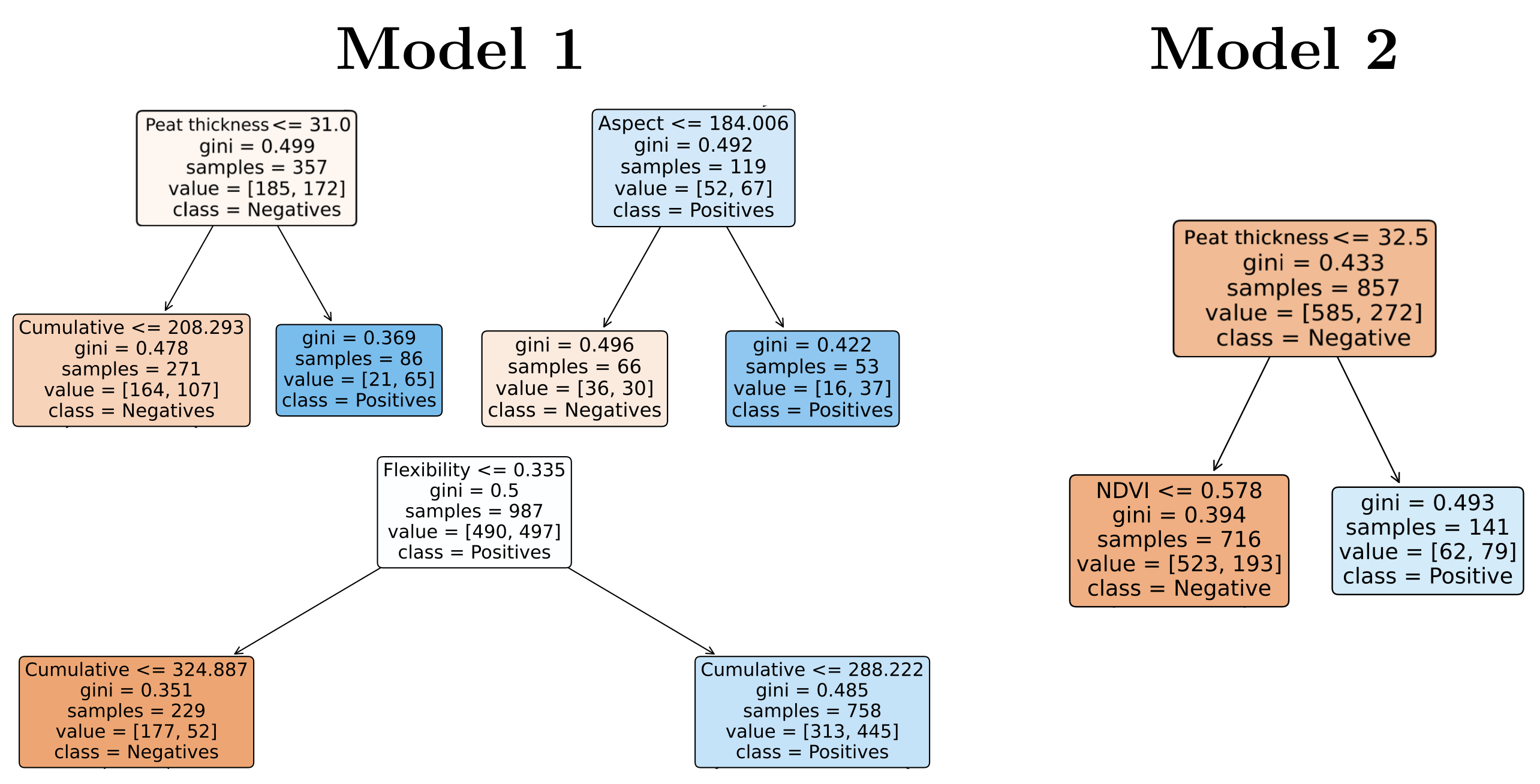
Figure 11 displays the generated decision tree constructed for Model 1 (cracks with a length greater than 2 m are considered as positives). All nodes split the observations upon ‘less than’ criteria, corresponding to one particular proxy. Whenever the considered proxy value of an observation meets this criterion, the observation is assigned to the left branch. By following the nodes, an observation eventually ends within a root node, classifying it as either a positive or negative. Along with the criterion, the remaining number of observations is given, the amount of positives against negatives and the Gini impurity. The Gini impurity of a node is also indicated by the intensity of the color of nodes. Intensely orange nodes are nodes containing a large number of negatives samples, while intensely blue nodes are nodes containing a large number of positive samples.

For Model 2, the exercise of pruning led to a tree with a depth of 4 (see Figure 12). The top node of the decision tree, which is for this model split upon the precipitation deficit, is now characterized by a Gini impurity of exactly 0.5. This value represents the most impure node. This is due to an oversampling technique, as it resulted in an equal number of positives and negatives.

In general, it can be observed that Model 2 performs better at splitting the positives and negatives, as the top node is split into nodes that clearly are orange and blue. After the first split, the colors hold on consistently, except for the blue node in the orange branch after being split upon the peat thickness. Both trees indicate that the positives and negatives can be split upon the peat thickness, as peat thickness values greater than 31 (Model 1) and 32.5 (Model 2) are associated with positives. Splitting upon the aspect in Model 1 results in a separation into a orange and blue node, which is not observed in Model 2. The node in latter model splits an already blue node, however, limiting the separative capacity of the proxy. Additionally, it is seen that in both models, the precipitation deficit splits the observations in the same manner, as positives are in both cases associated with high precipitation deficit values. An important difference, however, is that Model 1 first splits upon the soil flexibility, whereas Model 2 first splits upon the precipitation deficit.

This suggests that according to the data, no long cracks are observed upon levees with a flexibility lower than 0.335 m/kPa. Exceedance of the soil flexibility leads the database to a split upon the precipitation deficit. Non-exceedance does not seem to imply negatives, as a peat thickness of at least 31 cm may still induce cracking. This value of the peat thickness is close to the peat thickness value of 32.5, as seen in Figure 12, corresponding to Model 2. This suggests that, both for long cracks and cracks in general, this minimum peat thickness value is an important proxy when identifying crack-prone levees.

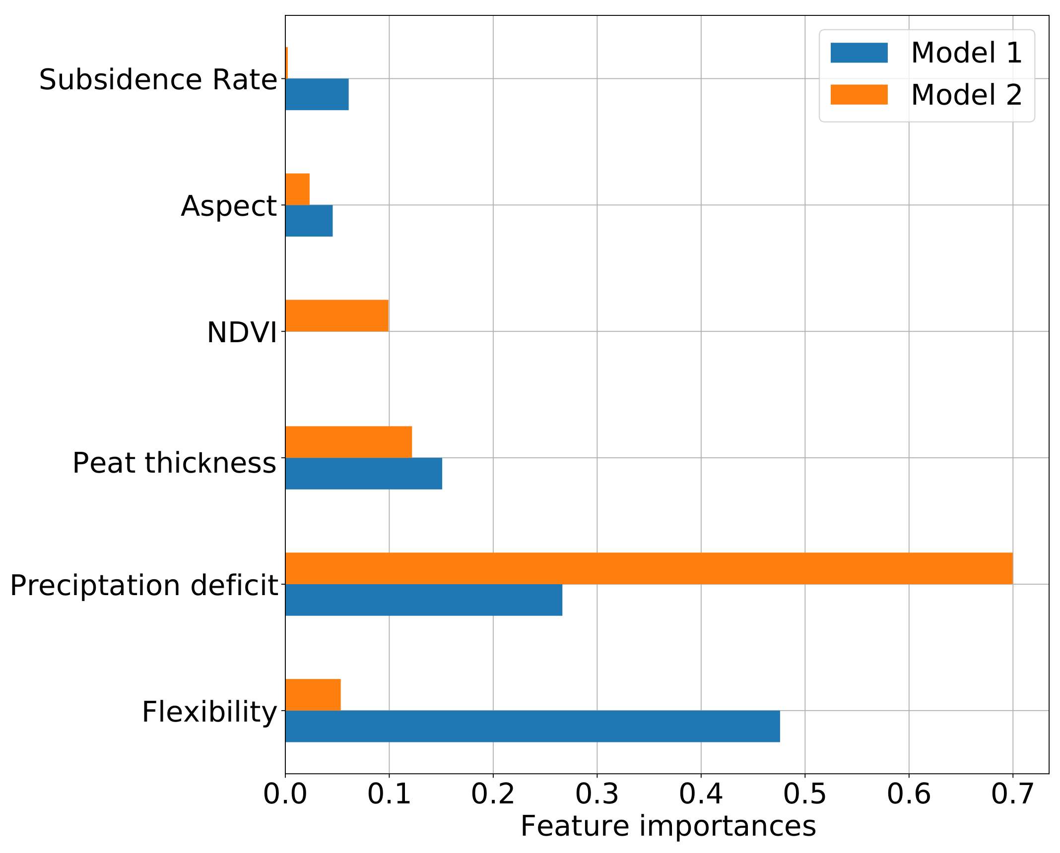
Figure 13 displays the feature importances of the proxies within the decision tree. It is observed that the precipitation deficit is quantified with the highest feature importance in the case of Model 2. For Model 1, it is observed that the soil flexibility is quantified with the highest feature importance. The soil flexibility is quantified with a feature importance of 0.05 in the case of Model 2. The feature importances also indicate that the NDVI is significant for Model 2 only. It seems that the peat thickness holds almost equal feature importance for both models. This indicates that the soil flexibility performs better at predicting positives in Model 1, in which large cracks are considered. This indicates that the occurrence of large cracks can be predicted better by understanding the soil flexibility of levees. Cracks in general, however (in Model 2), are more easily separated from non-cracks by the precipitation deficit.

Table 2. Performance indicators for Model 1 and Model 2.

	Model 1	Model 2
Train set accuracy	0.64	0.77
Test set accuracy	0.68	0.73
Precision	0.82	0.89
Recall	0.68	0.60
MCC	0.31	0.51
Cross validation accuracy	0.59	0.67

shows the indicators computed for both models. It can be seen that, in general, Model 2 performs better than Model 1. This is in accordance with the correlations which were observed in Figure 8. The better performance of Model 2 can be explained by the extremely high feature importance of the precipitation deficit, as seen in Figure 13. Model 2 can, therefore, attain good separation between the observations using only the data of one proxy variable, whereas Model 1 requires the data of multiple proxy variables. The requirement of multiple proxy variables increases the number of required splitting nodes, which increases the likelihood that samples contain data that cannot be split easily. This results in less pure nodes and hence a lower performance.

Figure 14 depicts the confusion matrices for both models, both in absolute values and normalized values. From left to right, top to bottom, are the TN, FP, FN and TP given. Large values in the diagonals are, therefore, preferred, as this increases the performance of the models.

It is seen that Model 1 performs slightly better at predicting positives than in the case of Model 2. Model 2, however, performs significantly better at predicting negatives. Since Model 2 cumulatively performs better at predicting either negatives or positives, the performance of the model is evaluated with a greater value of the MCC (see Table 2).

5.3. Hazard Indicators

Hazard indicators were extracted from the decision trees corresponding to both models. Hazard indicators for Model 1 concerned the peat thickness, the aspect and the soil flexibility. For Model 2, only the peat thickness was defined as a hazard indicator. Figure 15 display the hazard indicators as single-node decision trees.

5.4. Hazard Maps

Figure 16 shows the constructed maps for both models. Since the model tree of Model 2 only resulted in one hazard indicator, levees satisfying that indicator were highlighted. In the figures below, the color scale represents the amount of sampled points which were projected upon the levee segments after the points were assigned the hazard indicator data and potentially eliminated. For example, a sampled point which was located upon a coordinate characterized by a peat thickness smaller than 31 centimeters (see Figure 15) was eliminated. If a levee segment is characterized by a value of 4, this implies that four remaining points were projected onto that specific segment after the elimination procedure.

Figure 17 shows the empirical hazard maps and the Delfland ranks for comparison against the hazard maps constructed using the model trees.

The empirical hazard map (see Figure 17) shows that fewer levees are indicated as hazardous when compared with the hazard map constructed from Model 1. It is, however, important to understand that cracks are only observed on levees where inspections are conducted, potentially leading to a confirmation bias. The hazard map corresponding to Model 1 does suggest that more levees might be prone to cracks than considered by HHD at the current moment. From Figure 16, we observe that more extreme crack-prone regions according to Model 1 coincide with the crack-prone regions according to Model 2. This may, however, be due to the fact that the peat thickness and soil flexibility cannot be seen as independent variables. Notice that the constructed hazard maps were constructed with deterministic, static variables, as the precipitation deficit and NDVI are represented by stochastic variables which are hard to predict. As an improvement on this model, accurate weather forecasting can be used in order to use the model for real-time operational hazard-based asset management.

6. Discussion

The identification of proxy variables directly related to the cracking mechanism and the identification of potential cracking locations yields insights which add to our understanding of the drought-induced crack-proneness of levees. The identification of the proxy variables mainly focuses on describing the moisture content and the moisture content at cracking. Since the precipitation deficit was calculated with the Makkink evaporation, the temperature and radiation were already taken into account. For the purpose of improving the quality of this research, while potentially decreasing the required amount of data and data processing, it is advised to investigate the possibilities of applying databases in which the soil moisture content itself is expressed on a regional scale.

Figure 8 shows the impact of varying the period over which the precipitation deficit is calculated to optimize distinctiveness between expecting cracks and expecting no cracks. The curves display peaks at two different locations. The two peaks also differ in Cramérs V, resulting in a better performance of Model 2. From this, we learn that a period of 4 days should be used for the prediction of levees with long cracks, whereas a period of 123 days should be used for the (better) prediction of levees with cracks in general. The figure shows that periods longer than 200 days cannot distinguish between positives and negatives. This observation could be explained by the fact that 200 days prior to April (start of dry period according to HHD), the levees are exposed to winter conditions. Model 2 shows a higher optimal Cramérs V than Model 1. One might argue that cracks in general are then easier to predict solely based on precipitation deficit (also given the higher MCC of Model 2), however, this greater value might also be due to the application of an oversampling technique. Sampling negatives over periods in which cracks were not observed may as well have sampled them in drier periods, which automatically distinguishes positives in wetter periods and negatives in dryer periods.

Figure 9 shows that the most important factor identified in this study for the cracking process is the precipitation deficit, as both observation states 1 and 2 are best correlated with that proxy. This complies with the observation that the volumes of cracks tend to increase during dry periods [3], as cracks with large dimensions are more likely to be observed during inspection. After the precipitation comes the soil flexibility, which is the second best correlated with both observation states. We observe from Figure 10 that these higher Cramérs V values originate from the clearest distinction between positives and negatives, especially valid for the precipitation deficit. Positives are characterized by higher precipitation deficits, while negatives are characterized by lower precipitation deficits, which is an expected result. The high associations among the subsidence rate, peat thickness and soil flexibility themselves could be due to the fact that the databases contain mutual information, as a high peat thickness should be correlated with the soil flexibility from a physical point of view.

For Model 1, it is important to notice that an aspect of 184 degrees is defined as a hazard indicator, as this value indicates that the slope of the levees is directed southwards towards the sun (for most of the day). Model 2 shows that for a precipitation deficit of at least 331 cm, all observations in the database are defined as positives. This is unexpected, as this implies that all levees would be expected to crack. This may be due to the arbitrary definition of the dimensions of the cracks, implying that expected cracks might be characterized by dimensions in the order of millimeters. Since it is assumed that these dimensions do not pose a hazard to levee stability, it is not preferred to predict those. Proper insight into the relationship between crack dimensions and levee stability decrease will contribute to a machine learning framework in which the focus lies more on risk instead of only hazard. According to the performance indicators displayed in Table 2, Model 2 performs better with respect to all indicators. However, this high performance may be due to the combination of the random sampling of negatives and the oversampling techniques. Since the (sampled) negatives formed the minority of the database, random sampled observations were used as a basis for the oversampling technique. Obtaining validated negatives (by inspectors) might help to avoid such errors in the future. Despite the fact that Model 1 performs worse at the performance indicators, from Figure 14, we observe that Model 1 performs better at true positives. This is a desired property, as we aim to identify crack-prone levees.

As the dimensions of the cracks in general are arbitrary, this may imply that cracks with dimensions in the order of millimeters may also occur on the levees. This implies that accurate monitoring of the peat thickness and soil flexibility allows for a spatial understanding of the crack-proneness of levees. When this information is combined with real-time monitoring of the spatial precipitation deficit, the model trees can be utilized for operational hazard-based asset management of the levees. An investigation in the field was organized as a first attempt to validate the findings of the model trees. The investigation was conducted during the winter season and no (remnants of) cracks were observed on the levees defined as hazardous by both the model trees and on which cracks were observed more frequently during inspections. From this, we can conclude that the cracks close during the winter season, from which we learn that asset management focused on drought-induced cracks should be performed during a defined dry season. This season may be a fixed period of the year, but it is advised to define this according to the precipitation deficit values found in the model trees. As the trees indicate that a precipitation deficit of approximately 300 mm acts as a hazard indicator, it is advised that inspections focused on drought begin when this value is observed for an arbitrary coordinate. During the dry season, it is advised that the absence of cracks on levees is registered as well in order to obtain a database with reduced likeliness of false negatives. At last, when levees are not inspected frequently in the dry season while the model tree defines them as hazardous, they should be inspected to verify the crack-proneness. When this is not the case, the inspections result in true negatives that can be used to update the model trees.

7. Conclusions

A method for building a data-driven model is presented which helps to predict levees prone to cracking by combining observational available databases with local environmental factors, which where found to correlate best with the cracking physical process. Proxies were identified which correlated best to a levee cracking observational dataset without necessarily implying causation. We present different correlation studies to understand how the precipitation deficit and the flexibility of a soil allowed us to identify them as important proxies for the prediction of the cracking process. The precipitation deficit, for example, was calculated approximately between periods of 5 and 120 days prior to the date of observation, which showed the highest correlation with the occurrence of the general and long crack types, among all evaluated potential proxies. The correlation study showed that a cumulative precipitation deficit period of 123 days is best at predicting the occurrence of cracks in general, while a period of 4 days is found for longer, stability-endangering cracks.

Based on the obtained model trees of the data driven model, it was concluded that long cracks are not observed on levees for which the soil flexibility was smaller than 0.355 m/kPa, while this is not the case for cracks in general. In addition, the data show that longer cracks are more often found on levees of which the slope is oriented towards the southern side. For both longer cracks and cracks in general, the model trees state that a peat thickness of the upper layer of at least 31 cm indicates that levees are susceptible to the formation of cracks. Levees composed of soils which have peat layers thinner than 31 cm do not seem to crack for precipitation deficit values lower than 311 mm.

The model trees indicate that insight in the peat thickness, the orientation of the levee and the soil stiffness can be used as easily quantifiable proxies to identify areas that are prone to longer cracks. The model trees also show that for crack susceptibility in general, insight in the peat thickness suffices (with the precipitation deficit being a highly indicative, but not easily quantifiable proxy).

References

1. Attema, J.; Bakker, A.; Beersma, J.; Bessembinder, J.; Boers, J.; Brandsma, T.; van den Brink, H.; Drijfhout, S.; Eskes, H.; Haarsma, R.; et al. KNMI’14: Climate Change Scenarios for the 21st Century–A Netherlands Perspective; Technical Report WR-2014-01; KNMI: De Bilt, The Netherlands, 2014. [Google Scholar]
2. Vardon, P.J. Climatic influence on geotechnical infrastructure: A review. Environ. Geotech. 2015, 2, 166–174. [Google Scholar] [CrossRef]
3. Jamalinia, E.; Vardon, P.J.; Steele-Dunne, S. The impact of evaporation induced cracks and precipitation on temporal slope stability. Comput. Geotech. 2020, 122, 103506. [Google Scholar] [CrossRef]
4. Van Baars, S. The horizontal failure mechanism of the Wilnis peat dyke. Géotechnique 2005, 55, 319–323. [Google Scholar] [CrossRef]
5. Vahedifard, F.; Robinson, J.; AghaKouchak, A. Can protracted drought undermine the structural integrity of California’s earthen levees? J. Geotech. Geoenviron. Eng. 2016, 142, 02516001. [Google Scholar] [CrossRef] [Green Version]
6. van den Akker, J.; Hendriks, R.; Frissel, J.; Oostindie, K.; Wesseling, J. Gedrag van Verdroogde Kades: Fase B, C, D: Onstaan en Gevaar van Krimpscheuren in Klei- en Veenkades; Number 2473 in Alterra-Rapport; Alterra: Wageningen, The Netherlands, 2014. [Google Scholar]
7. Yang, R.; Huang, J.; Griffiths, D.; Sheng, D. Effects of desiccation cracks on slope reliability. In Proceedings of the 7th International Symposium on Geotechnical Safety and Risk (ISGSR), Taipei, Taiwan, 11–13 December 2019; pp. 261–266. [Google Scholar] [CrossRef]
8. Aguilar-López, J.P.; Bogaard, T.; Gerke, H.H. Dual-permeability model improvements for representation of preferential flow in fractured clays. Water Resour. Res. 2020, 56, e2020WR027304. [Google Scholar] [CrossRef]
9. Wang, Z.F.; Li, J.H.; Zhang, L.M. Influence of cracks on the stability of a cracked soil slope. In Proceedings of the 5th Asia-Pacific Conference on Unsaturated Soils, Pattaya, Thailand, 14–16 November 2011; Volume 2, pp. 721–728. [Google Scholar]
10. Hallett, P.D.; Newson, T.A. Describing soil crack formation using elastic–plastic fracture mechanics. Eur. J. Soil Sci. 2005, 56, 31–38. [Google Scholar] [CrossRef]
11. Hoang, N.D.; Nguyen, Q.L. A novel method for asphalt pavement crack classification based on image processing and machine learning. Eng. Comput. 2019, 35, 487–498. [Google Scholar] [CrossRef]
12. Al-Ruzouq, R.; Shanableh, A.; Yilmaz, A.G.; Idris, A.; Mukherjee, S.; Khalil, M.A.; Gibril, M.B.A. Dam site suitability mapping and analysis using an integrated GIS and machine learning approach. Water 2019, 11, 1880. [Google Scholar] [CrossRef] [Green Version]
13. Jamalinia, E.; Tehrani, F.S.; Steele-Dunne, S.C.; Vardon, P.J. A Data-Driven Surrogate Approach for the Temporal Stability Forecasting of Vegetation Covered Dikes. Water 2021, 13, 107. [Google Scholar] [CrossRef]
14. Zhu, M.; Li, S.; Wei, X.; Wang, P. Prediction and Stability Assessment of Soft Foundation Settlement of the Fishbone-Shaped Dike Near the Estuary of the Yangtze River Using Machine Learning Methods. Sustainability 2021, 13, 3744. [Google Scholar] [CrossRef]
15. Stark, T.; Jafari, N.; Leopold, A.; Brandon, T. Soil Compressibility in Transient Unsaturated Seepage Analyses. Can. Geotech. J. 2014, 51, 858–868. [Google Scholar] [CrossRef]
16. Camporese, M.; Ferraris, S.; Putti, M.; Salandin, P.; Teatini, P. Hydrological modeling in swelling/shrinking peat soils. Water Resour. Res. 2006, 42, W06420. [Google Scholar] [CrossRef] [Green Version]
17. Pyatt, D.G.; John, A.L. Modelling volume changes in peat under conifer plantations. J. Soil Sci. 1989, 40, 695–706. [Google Scholar] [CrossRef]
18. Fredlund, D.G. Consolidation and swelling processes in unsaturated soils. In Unsaturated Soil Mechanics in Engineering Practice; John Wiley & Sons, Inc.: Hoboken, NJ, USA, 2012; Chapter 16; pp. 809–857. [Google Scholar] [CrossRef]
19. World Meteorological Organization (WMO); Global Water Partnership (GWP). Handbook of Drought Indicators and Indices; Technical Report; Integrated Drought Management Programme (IDMP), Integrated Drought Management Tools and Guidelines Series 2; WMO: Geneva, Switzerland; GWP: Geneva, Switzerland, 2016. [Google Scholar]
20. Makkink, G.F.; Van Heemst, H.D.J. Potential evaporation. In Mededelingen; Instituut voor Biologisch en Scheikundig Onderzoek van Landbouwgewassen: Wageningen, The Netherlands, 1970. [Google Scholar]
21. Lu, J.; Sun, G.; McNulty, S.G.; Amatya, D.M. A Comparison of Six Potential Evapotranspiration Methods for Regional Use in the Southeastern United States. JAWRA J. Am. Water Resour. Assoc. 2005, 41, 621–633. [Google Scholar] [CrossRef]
22. Gerten, D.; Schaphoff, S.; Haberlandt, U.; Lucht, W.; Sitch, S. Terrestrial vegetation and water balance—Hydrological evaluation of a dynamic global vegetation model. J. Hydrol. 2004, 286, 249–270. [Google Scholar] [CrossRef]
23. Peters, A.J.; Walter-Shea, E.A.; Ji, L.; Viña, A.; Hayes, M.; Svoboda, M.D. Drought Monitoring with NDVI-Based Standardized Vegetation Index. Photogramm. Eng. Remote Sens. 2002, 68, 71–75. [Google Scholar]
24. Peng, X.; Horn, R. Identifying Six Types of Soil Shrinkage Curves from a Large Set of Experimental Data. Soil Sci. Soc. Am. J. 2013, 77, 372–381. [Google Scholar] [CrossRef]
25. Erkens, G. Draagkracht-Zettingsgevoeligheid, 2010, Deltares-1208234-DANK-024a. Available online: https://data.overheid.nl/en/dataset/26216-draagkracht—zettingsgevoeligheid (accessed on 30 September 2019).
26. Cramér, H. Mathematical Methods of Statistics (PMS-9); Princeton University Press: Princeton, NJ, USA, 2016. [Google Scholar] [CrossRef]
27. Rutkowski, L.; Jaworski, M.; Pietruczuk, L.; Duda, P. The CART decision tree for mining data streams. Inf. Sci. 2014, 266, 1–15. [Google Scholar] [CrossRef]
28. Zhi, T.; Luo, H.; Liu, Y. A Gini impurity-based interest flooding attack defence mechanism in NDN. IEEE Commun. Lett. 2018, 22, 538–541. [Google Scholar] [CrossRef]
29. Pedregosa, F.; Varoquaux, G.; Gramfort, A.; Michel, V.; Thirion, B.; Grisel, O.; Blondel, M.; Prettenhofer, P.; Weiss, R.; Dubourg, V.; et al. Scikit-learn: Machine Learning in Python. J. Mach. Learn. Res. 2011, 12, 2825–2830. [Google Scholar]
30. Boughorbel, S.; Jarray, F.; El-Anbari, M. Optimal classifier for imbalanced data using Matthews Correlation Coefficient metric. PLoS ONE 2017, 12, e0177678. [Google Scholar] [CrossRef] [PubMed]
31. Chicco, D.; Jurman, G. The advantages of the Matthews correlation coefficient (MCC) over F1 score and accuracy in binary classification evaluation. BMC Genom. 2020, 21, 1–13. [Google Scholar] [CrossRef] [PubMed] [Green Version]
32. Beguería, S.; Vicente-Serrano, S.M.; Reig, F.; Latorre, B. Standardized precipitation evapotranspiration index (SPEI) revisited: Parameter fitting, evapotranspiration models, tools, datasets and drought monitoring. Int. J. Climatol. 2014, 34, 3001–3023. [Google Scholar] [CrossRef] [Green Version]
33. Cateni, S.; Colla, V.; Vannucci, M. A method for resampling imbalanced datasets in binary classification tasks for real-world problems. Neurocomputing 2014, 135, 32–41. [Google Scholar] [CrossRef]
34. Wolters, E.; Hakvoort, H.; Bosch, S.; Versteeg, R.; Bakker, M.; Heijkers, J.; Talsme, M.; Peerdeman, K. Meteobase: Online neerslag-en referentiegewasver-dampingsdatabase voor het Nederlandse waterbeheer. Meteorologica 2013, 1, 15–18. [Google Scholar]
35. De Bruin, H. Over referentiegewasverdamping. Meteorologica 2014, 1, 15–20. [Google Scholar]
36. GDAL/OGR Contributors. GDAL/OGR Geospatial Data Abstraction Software Library; Open Source Geospatial Foundation: Chicago, IL, USA, 2021. [Google Scholar]
37. Brouwer, F. BRO—Bodemkaart van Nederland, uri:0e4c899b-42b1-4654-906e-4ad2a8d838cb. 2018. Available online: https://www.dinoloket.nl (accessed on 30 September 2019).
38. Provincie Zuid-Holland. Veendikte 2014, uri:098B74D3-D49B-422A-BCA4-6C11A3FA7D2A. 2014. Available online: https://atlas.zuid-holland.nl/GeoWeb56/index.html?viewer=Bodematlas (accessed on 30 September 2019).
39. Jeevalakshmi, D.; Reddy, S.N.; Manikiam, B. Land cover classification based on NDVI using LANDSAT8 time series: A case study Tirupati region. In Proceedings of the 2016 International Conference on Communication and Signal Processing (ICCSP), Melmaruvathur, India, 6–8 April 2016; pp. 1332–1335. [Google Scholar] [CrossRef]
Figure 1. Cross sections where possible drought-induced failure mechanisms are illustrated. (A) shows the mechanism of horizontal sliding. (B,C) depict macro-instability and subsidence due to drought, respectively.
Sustainability 14 06820 g001
Figure 2. (A) shows the first stage of soil shrinkage due to drying conditions where only subsidence occurs. (B) shows the second phase, in which isotropic shrinkage [17] is expected.
Sustainability 14 06820 g002
Figure 3. The discussed potential proxies and their relevance with respect to levees.
Sustainability 14 06820 g003
Figure 4. Visual schematization of the methodology followed in this paper. A data-based understanding of the spatial distribution of crack-prone levees is manifested in the form of hazard maps. The subparagraph in which the element indicated in the figure is elaborated upon more thoroughly is shown between parentheses.
Sustainability 14 06820 g004
Figure 5. A graphical representation of the manner in which the proxy data were assigned to the observations. The left figure depicts that the observations (both positives and negatives) are evaluated on their spatiotemporal coordinates to extract precipitation deficit time-series for all observations in the database. In the figure, three rasters (corresponding to the 3 days) are shown. In reality, however, 5 years’ worth of data was extracted. The right figure depicts that the observations were only evaluated on their spatial coordinates in order to extract and assign the remaining proxy data. Multiple NDVI rasters were retrieved, however, since the NDVI is a time-dependent proxy. For every observation, the NDVI raster generated on the nearest date (in time) was evaluated. In this manner, a single value was assigned to the observations, where the precipitation deficit data were assigned as a time-series to the observations.
Sustainability 14 06820 g005
Figure 6. The figure depicts a database in which all instances are associated with an x value. The left side of the image shows a small decision tree in which a split is defined such that only pure nodes are left. This is a perfect split as the resulting nodes are both evaluated with a Gini impurity of 0. Since no further decrease in impurity can be gained, the resulting nodes are not split subsequently. The right side shows a small decision tree in which no decision rule can be defined that decreases the average Gini impurity of the resulting nodes. The node is, therefore, not split. The color of a node indicates whether the majority is made up of positives (blue) or negatives (orange). The intensity of the color represents the purity of the node.
Sustainability 14 06820 g006
Figure 7. (A) presents locations of observed cracks during drought inspections conducted in the years 2018, 2019 and 2020. (B) presents the inspected levees during the dry periods per rank. The boundaries of the area which is administered by HHD are shown in black.
Sustainability 14 06820 g007
Figure 8. Cramérs V plotted against the period over which the cumulative precipitation deficit is calculated. A high value indicates a clear distinction between positives and negatives. The curves show a similar form, in which an obvious peak is observed (period of a few days). Between a period of 100 and 200 days, an almost constant Cramérs V is observed, indicating that this interval is equally adequate for separating positives from negatives.
Sustainability 14 06820 g008
Figure 9. Heat map displaying the Cramérs V correlations. Observation state represents the state of the observations according to Model 1 or 2.
Sustainability 14 06820 g009
Figure 10. Scatter plots for all numerical values representing the proxy variables. The axes depict the proxies that are plotted against one another. The diagonals depict the histograms of the individual proxy variables (observation state according to Model 1). Note that the values of the subsidence rate have been multiplied by 10 6 for visual purposes.
Sustainability 14 06820 g010
Figure 11. Decision tree corresponding to the prediction of positives and negatives (according to Model 1). The precipitation deficit is shown with ‘Cumulative’ in the figure (as well as in Figure 12). The colors indicate whether the positives (blue) or negatives (orange) make up the majority of the node. The intensity of the color indicates the purity of the node. White nodes (the first ones) are therefore quantified by a high Gini impurity. From this model tree, it is observed that the tree becomes balanced after the first split to the right. From this, we learn that cracks larger than 2 meters are not observed on soil bodies characterized by a low flexibility.
Sustainability 14 06820 g011
Figure 12. Decision tree corresponding to the prediction of positives and negatives (according to Model 2). The colors indicate whether positives (blue) or negatives (orange) make up the majority of the node. The intensity of the color indicates the purity of the node.
Sustainability 14 06820 g012
Figure 13. Feature importances corresponding to the decision tree. The horizontal axis denotes the relative weight of proxies in classifying the samples.
Sustainability 14 06820 g013
Figure 14. Confusion matrices for both models. The top two matrices show the regular matrices, whereas the bottom two show normalized matrices. The values are normalized with respect to the sum of the horizontal cells.
Sustainability 14 06820 g014
Figure 15. Hazard indicators corresponding to Model 1 and Model 2, which were extracted from the constructed tree models. The above-shown proxy variables are easily predictable in time (due to their constant-in-time character, hence, they are defined as hazard predictors (the range that leads to positives)). Levees situated on soils that meet these criteria are expected to be prone to drought-induced cracks.
Sustainability 14 06820 g015
Figure 16. Hazard maps for Model 1 (left) and Model 2 (right). In Model 1, hazard is quantified with numbers. Large numbers represent crack-prone levees, whereas a value of 0 is associated with complete absence of proneness. Model 2 performs a binary classification, in which the red levees are defined as crack-prone.
Sustainability 14 06820 g016
Figure 17. The left image shows the constructed empirical hazard map. The right image shows the Delfland ranks for comparison with the other maps.
Sustainability 14 06820 g017