Abstract
Residential electricity consumption is an important part of the electricity consumption of the whole society. The systematic analysis of the influence mechanism of the external complex factors of residential electricity consumption is significant for scientific and effective power demand side optimization management. From the socio-economic and climate perspectives, Spearman’s correlation was used to analyze external multiple disturbance indicators, and principal component analysis (PCA) was used to reduce data dimensionality. The multi-factor residential electricity measurement model (PCA-MCA) was established to explore the heterogeneity of influence mechanisms. Taking Beijing as a case study, the results show that the sensitivity of residential electricity consumption of Beijing to socio-economic indicators is greater than that of climate indicators, and the two influencing factors are obviously heterogeneous. The impact of socio-economic factors on residential electricity consumption appears to have continuous and stable characteristics, but climate factors are more volatile. This paper discusses factors and disturbance mechanisms of regional residential electricity consumption, fully considering the actual situation in Beijing. Taking the realization of regional power demand lateral optimization management as the idea, the paper proposes some optimization strategies to achieve regional power availability. This provides an analysis basis and practical reference for sustainable development of regional power.
1. Introduction
In recent years, with the continuous development of social production and living standards, the proportion of residential electricity consumption in the total energy consumption of society has gradually increased from 10.53% in 1996 to 14.2% in 2019. Compared with previous years, it is currently showing a trend of rapid growth, surpassing the growth rate of electricity consumption in other parts of society during the same period. Therefore, it is of realistic meaning to conduct in-depth research on the influence factors of residential electricity consumption.
On the one hand, China’s actual situations have led to problems such as large volume of electricity consumption by Chinese residents and uneven regional supply and demand. In terms of residential electricity consumption, residential electricity consumption behavior determines the size of residential electricity consumption. China is the most populous country in the world, accounting for about 20% of the world’s population. The large population is one of the main reasons for the large amount of electricity consumption [1,2]. Income guides residential consumption behavior and is one of the main influence factors that affect residential electricity consumption [3]. It can be seen intuitively from Figure 1 that since 1996, China’s residential electricity consumption, population, and income have all shown an increasing trend. In 2018, the electricity consumption of Chinese residents was about 8.55 times that of 1996, the population was about 1.14 times that of 1996, and the income was about 8.11 times that of 1996. It can be seen that both residential electricity consumption and income have developed rapidly, and as shown in Figure 1, the growth rates of the two are roughly the same. From another perspective, the use of various household appliances, such as lighting and cooling in residential homes, is one of the main sources of electricity consumption [4]. The carbon emissions caused by electricity production have a great impact on the greenhouse gas effects and worsen the climate [5,6]. In the Paris Agreement, it is pointed out that developing countries such as China and India should improve emission reduction targets according to their own conditions and gradually achieve these. For China, the emission reduction target is even more urgent. From 1984 to 2018, the proportion of years where China’s annual temperature change rate was faster than that of the world was about 60%, indicating that China’s local climate change is more serious than the global one. According to the China Blue Book of Climate Change (2020), from 1951 to 2019, the annual average temperature of China increased by 0.24 °C every 10 years. Even the rate of temperature increase was significantly higher than the global average during the same period. Industrial development has led to a rapid increase in the concentration of carbon dioxide, bringing the urgency of the climate issue to a new level. The increase in extreme weather in China has increased the dependence of residents on household appliances [7,8], which makes a huge challenge to China’s emissions reduction targets in residential electricity consumption. Therefore, the residential electricity consumption problem of China must be analyzed and adjusted in a complete way to gradually adapt to the global emission reduction target.
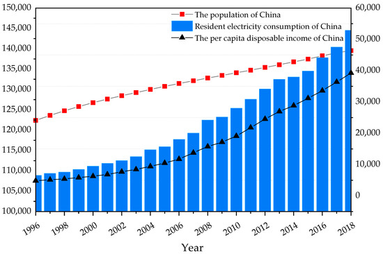
Figure 1.
Residential electricity consumption, the per capita disposable income and the population in China from 1996 to 2018. Source: National Bureau of Statistics of China.
On the other hand, the eastern coastal areas of China are densely populated, with more than 400 people per square kilometer, the central area is about 200 people per square kilometer and the western plateau areas are sparsely populated, with less than 10 people per square kilometer. Therefore, the areas of peak residential electricity consumption in China are concentrated, located in the east of China. Even though Shandong Province in eastern China ranks first in power generation in the country, its electricity consumption in the whole society far exceeds its power generation by more than 50 billion kWh, which cannot meet its own needs. Compared with other provinces in China, the Inner Mongolia Autonomous Region in northern China generated 147.53 billion kilowatt-hours of electricity in 2018. Sichuan Province in western China generated 103.96 billion kilowatt-hours of electricity in 2018. Therefore, most of the electricity consumption in the eastern and central regions of China is transmitted through the “West-to-East Power Transmission Project” and “North-To-South Power Transmission project” [9]. To a certain extent, it plays a role in optimizing the allocation of power grid resources [10]. Part of the power is wasted due to insufficient power infrastructure in China. In addition, the construction of China’s power grid is seriously lagging behind the power source construction. Power sources are surplus, and supply exceeds demand. At the end of 2015, the reserve capacity of China’s power market reached 38%. However, the power grid’s ability to optimize resource allocation is insufficient, and the power system is poorly adjustable, with less than 6% proportion of the flexibly adjustable power sources in installed capacity. This has become an important issue restricting the sustainable development of China’s power industry. Therefore, peak power demand can be reduced by strengthening the power demand side management, and power demand side management can alleviate supply shortages when power is lacking. Also, it can be used to adjust energy consumption structure when there is surplus. The two aspects of it can lay the foundation for achieving incremental substitution of electric energy.
A clear and accurate understanding of trends and influence factors of power demand will not only help the supply side make a reasonable and accurate power plan that has an effective management of demand side, but it also helps ensure the sustainable development of China’s power industry. Therefore, based on the above, this paper deeply discusses the factors that affect residential electricity consumption. We achieve the purpose of improving the accuracy of the model based on the principal component regression in Section 3. Furthermore, we analyze the heterogeneity of the socio-economic factors and the climate factors and focus on one case to propose optimized regional power demand side management in Section 5. Through the discussion in this article, the power sector can have a better understanding of the factors that affect residential electricity consumption, so as to better arrange power planning and optimize the allocation of power resources.
2. Literature Review
In recent years, the research results of residential electricity consumption are very rich. These mainly focus on the analysis of single influence factors and the optimization of residential electricity measurement models.
(1) Factor-analysis of single dimension. Related research focuses on the impact of a single factor on residential electricity consumption or residential load. At the socio-economic level, Fintan McLoughlin et al. discussed the four socio-economic factors based on multiple linear regression models, and the results showed that the income effect makes high-income people have greater power demand [11]. Zhou and Teng found that the scale of housing and the holding of household appliances are also important determinants of residential electricity demand [12]. Many scholars have used the method of autoregressive distribution to study electricity demand and found that electricity demand is mainly determined by income and economic development level and has a weak relationship with electricity prices [13,14,15]. Shibano and Mogi proposed a household income electricity consumption model to estimate the electricity consumption of residents in a specific area [16]. Aydin and Brounen analyzed the impact of residential energy-saving policies on the electricity consumption of European residents from 1980 to 2016 and found that the energy label requirements of electrical appliances and stricter building regulations have led to a decline in residential electricity consumption [17]. HaHyun et al. used population polynomials to illustrate the impact of population age distribution on the electricity consumption of Korean residents and found that the population of 20–44 years old and over 60 increased residential electricity consumption [18]. At the level of climate factors, Alberini et al. decomposed the factors that affect residents’ daily electricity consumption into four parts, starting from the selection of time period and temperature range, and focused on the mechanism of climate impact on Italian residential electricity consumption [19]. Allen et al. found that in the next 40 years, the increase in electricity demand caused by rising temperatures will have the greatest impact on less populated areas [20]. Auffhammer et al. combined 20 downscaling global climate models with temperature response functions to predict the impact of climate change on total daily consumption and daily peak loads [21]. Shourav et al. found that temperature and precipitation have an impact on daily electricity consumption [22]. Franco and Sanstad used many climate scenarios to predict the concentration of carbon dioxide in California, and simulated the maximum temperature per hour, fitting the function relationship between hourly power demand and hourly maximum temperature [23]. Song et al. normalized the specific daily power demand into the relationship between the basic power demand and temperature, and calculated the temperature sensitivity every 3 h, reducing the prediction error of the special daily load [24]. Mukhopadhyay and Nateghi used the Bayesian additive regression tree method to capture the complex structure of the data and concluded that the average dew point temperature is more suitable for predicting climate-sensitive loads than the most commonly used average daily temperature, and wind speed and precipitation are key predictors for the climate-sensitive parts indicator [25]. Fumo and Biswas used multiple regression analysis methods to analyze the impact of outdoor temperature and solar radiation on residential electricity consumption [26].
(2) Residential electricity consumption measurement model. In recent years, with the development of technology, the power system has higher requirements for the stability of residential load, and accurate measurement of residential electricity is a key factor. Wang et al. proposed a set of prediction methods that combine the lasso algorithm with Gaussian process regression, which not only reduces the dimensionality of input data, but also improves the accuracy of model prediction [27]. Yang et al. used the panel data analysis method combined with the controlled variable method to quantitatively analyze the residential electricity consumption, so that the model results are true and reliable [28]. Blazquez et al. used the dynamic logarithmic demand function of the two-step system Gaussian Mixed Model (GMM) estimator to analyze the panel data of Spanish residential electricity consumption and innovated the use of panel data [29]. Based on the co-integration measurement method, Shahzad et al. proposed to use the rebound effect to measure the factors affecting the residents’ load and separated the short-term model from the long-term model to eliminate the deviation caused by the time period [30]. Based on optimal subset regression and the Mann-Kendall (M-K) test, Zheng et al. comprehensively demonstrated the changing trend of electricity consumption of Guangzhou residents under various conditions under different socio-economic paths and carbon dioxide concentrations [31]. Liu et al. proposed a hybrid model for ultra-short-term forecasting of residential electricity consumption based on exponential smoothing and extreme learning machines, which usually has low errors [32]. Hussain and Maha used the Driving forces-Pressures-State-Impacts-Responses (DPSIR) model to fully consider the driving factors for the growth of residential electricity consumption and improve the accuracy of the model [33]. Elkamel et al. applied a multiple regression model and three convolutional neural networks to predict the electricity consumption of Florida residents, and the results showed that the multi-channel neural network that took all time series variables into account had the highest accuracy [34]. Khan et al. integrated a convolutional neural network and a multi-layer bidirectional gated recurrent unit into a deep learning hybrid model, and the error rate of the dataset of this model was greatly reduced [35]. Ngabesong and McLauchlan used the R language to realize the accurate prediction of the electricity demand in Texas. The time series model was processed and implemented in the R planning environment, and it can be used for random analysis and future electricity demand forecasting [36]. Saravanan et al. proposed two forms of genetic algorithms to estimate power demand, select the best-fitting genetic algorithm model based on the average error percentage, and make more accurate predictions of power demand under different scenarios [37]. Ningpramuda et al. used dynamic simulation methods to discuss the dynamic behavior of current and future power demand based on three scenarios and provided a flexible solution for future power demand forecasting [38]. Sowinski proposed a power demand forecasting method based on the idea of the end-use model, taking regional power consumption and population growth forecasts as input, and outputting the forecast results of mid-term power demand levels [39]. Using limited historical data, Kartikasari et al. used the dual moving average model, the Holt exponential smoothing model, and the Grey model (GM) (1,1) model to predict the electricity demand in Indonesia. The results showed that the gray GM (1,1) model has the smallest error. The fitting effect is the best [40]. Serge et al. created a new GM (1,1)-VAR (1) hybrid model based on Vector Auto regression (VAR) and Grey models to predict residential electricity consumption in Cameroon, with a root mean square error of 1.628% [41].
From the review of documents, it can be seen that for the current electricity market in China, the research on residential electricity consumption is mainly concentrated on the socio-economic level. Although the climate factors with increasing influence are involved, there is less discussion on factors outside the residents. Under the current situation, there are two major issues that need to be considered: (1) How to take all necessary influence factors into consideration to obtain accurate residential electricity consumption, and (2) whether there is heterogeneity among the influence mechanisms of various factors, and if there is heterogeneity, how to measure residential electricity consumption, respectively. Only by scientifically resolving the questions can we have a deeper understanding of the influence factors of electricity consumption, which makes us more targeted on power demand side management. This will help to achieve the sustainable development of China’s power industry. Therefore, this paper analyzed the mechanism of multiple indicators affecting electricity consumption outside the resident and performed data dimensionality reduction processing on the basis of ensuring data integrity. Through the above, we constructed a high-precision and multi-factor residential electricity measurement model to predict accurately. The factors mentioned above can guide the optimization of power demand side management.
3. Methodology
In this paper, a multi-factor residential electricity consumption model was constructed from two perspectives to extract indicators that measure the socio-economic factors and the climate factors. By analyzing the Spearman correlation degree of the indicators, we eliminated the indicators that were not highly relevant. Principal component analysis (PCA) was used to reduce the dimensions of the data, extract the top four principal components of the variance contribution rate, and establish the multi-factor residential electricity consumption function. With it, this paper discussed the heterogeneity of two factors on the mechanism of residential electricity consumption. Finally, combined with the actual situation on the demand side and the supply side in Beijing, some optimal strategies were put forward to help optimize the allocation of resources in Beijing. The methodology of this research is shown in Figure 2 and the main research methods are systematically introduced below.
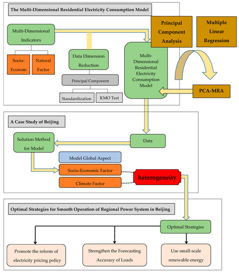
Figure 2.
The study process of the multi-dimensional residential electricity consumption model.
3.1. Method
This research aimed to examine the quantitative relationship between the residential electricity consumption of Beijing and the multi-dimensional influence factors. Because there is multi-collinearity in the indicators of the socio-economic and climate perspectives, and the data is in high dimensions, the principal component analysis is used to solve the multi-collinearity problem and reduce the dimension of the data [42].
3.1.1. Principal Component Analysis
In order not to be affected by the dimension of the original data, all data should be standardized as follows: zy, , , , , , , . The Kaiser-Meyer-Olkin (KMO) test is conducted on the data to observe whether it conforms to the conditions for principal component analysis:
The value of the KMO test changes from 0 to 1, and the larger the number of KMO sampling appropriateness, the more suitable for principal component analysis. When the KMO value is 0.5, it is not suitable for subsequent principal component analysis; when the KMO value is 0.7, it is suitable for principal component analysis.
Observe the data after standardization in the previous section and perform this step if it is suitable for principal component analysis. Principal component extraction is performed on standardized data, and principal components whose variance contribution rate was greater than 85% were extracted. The component matrices of these principal components were named matrix A and their eigenvalue moment B, then the matrix C used for subsequent calculations was equal to AB. Matrix C is a linear combination of all initial independent variables, as shown in Equation (2):
3.1.2. Multiple Regression Analysis: PCA-MCA
The matrix C and the standardized dependent variables were analyzed by least squares regression [43]. After the reduction of Equations (3) and (4), the final PCA-MCA multi-factor residential electricity metering Function (5) is obtained.
3.2. Data Sources
The global annual average surface temperature comes from the website of the National Oceanic and Atmospheric Administration on climate change (https://www.climate.gov/ accessed on 15 February 2021). The annual average temperature in China is from the “China Climate Bulletin” (1984–2018) and obtained from the China Meteorological Administration (http://www.cma.gov.cn/ accessed on 15 February 2021). China’s population, per capita disposable income of urban residents, and household electricity consumption are derived from the “China Statistical Yearbook” (2000–2018), obtained from the National Bureau of Statistics (http://www.stats.gov.cn/ accessed on 15 February 2021).
This paper is based on a case study in Beijing, and the residential electricity consumption of Beijing, annual maximum temperature, annual average temperature, permanent population, regional GDP, per capita disposable income, per capita regional product, resident consumption level, and social labor rates are all from the “Beijing Statistical Yearbook” (1999–2018), obtained from the Beijing Municipal Bureau of Statistics (http://tjj.beijing.gov.cn/ accessed on 15 February 2021). Weather-related data, such as average high-temperature days, high-temperature days, average relative humidity, precipitation, wind speed, and sultry index, all come from the Beijing Meteorological Station 54511, obtained from the National Greenhouse Data (http://data.sheshiyuanyi.com/WeatherData/ accessed on 15 February 2021). The average high-temperature days are the days when the daily average temperature is greater than 20 degrees Celsius, and the high-temperature days are the days when the daily maximum temperature is greater than 35 degrees Celsius. The sultry index is calculated from the daily average temperature and average relative humidity.
4. The Multi-Dimensional Residential Electricity Consumption Model: A Case study Based on Beijing
4.1. Introduction of Residential Electricity Consumption in Beijing
Based on the future smart energy model, regional power demand side management is carried out with smart cities as the unit, so it is feasible to select cities for case studies in this paper [44]. As a representative of China’s megacities, the living standards of Beijing are higher than the average of China. It is a pioneer in the implementation of smart cities in the future, and its residential electricity consumption is large and unstable. How to achieve targeted power demand side management is very important for the sustainable development of regional power. As shown in Figure 3, the residential electricity consumption of Beijing rose from 30.78 million kWh in 1984 to 25,635.64 million kWh in 2018, an increase of approximately 35 times. In the situation of the continuous growth of electricity consumption, it is of great significance to conduct a deep research on the influence mechanism of electricity consumption in Beijing.
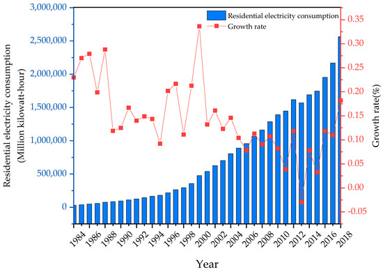
Figure 3.
Residential electricity consumption and growth rate in Beijing, China, from 1984 to 2018. Source: Beijing Municipal Bureau of Statistics.
On the demand side, the potential growth of residential electricity consumption in Beijing is huge, which brings great challenges to the supply side to accurately measure the electricity consumption. Residential electricity consumption behavior is affected by many factors, including socio-economic factors and climate factors [11,12,13,14,15,16,17,18]. With the improvement of people’s living standards, the people’s disposable income level has undergone tremendous changes. In 2019, the per capita disposable income of Beijing increased five times compared with 2000. The increase in disposable income has advanced the people’s level of demand. Use for electricity is no longer limited to the level of necessities. Secondly, climate change has intensified and disrupted Beijing’s climate self-regulation system. According to the research, by 2070, the North China Plain is very likely to become the center of heat waves [45]. Figure 4 reflects the increasing trend of annual average temperature and annual maximum temperature in Beijing over the past 30 years. After entering the 21st century, both rose to fluctuate within another range. As the temperature rises and the frequency of heat waves accelerates, the use time and frequency of cooling appliances continue to rise, which will lead to a rapid increase in residential electricity consumption.
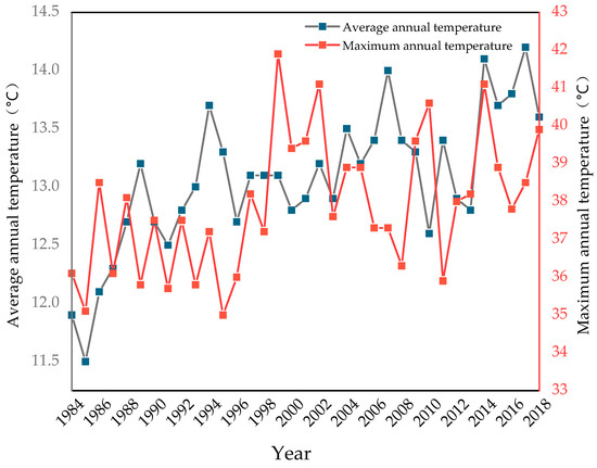
Figure 4.
The broken line chart of annual mean temperature of Beijing, China, from 1984 to 2018. Source: Beijing Municipal Bureau of Statistics.
For the supply side, the residential electricity load in Beijing is developing in a higher volume and is more diversified, which puts forward higher requirements for effective regional power demand side management. In recent years, the rapid development of Beijing’s economy and society has diversified the residential electricity load. The rapid growth of the load, the advancement of the peak time, and the delay of the valley time are not compatible with the current grid power structure of Beijing. The resource optimization poses a problem of how to effectively implement regional power demand side management and optimize the allocation of existing power grid resources under complicated situations, such as to large electricity volume, diversified loads, and unstable influencing factors [46,47]. Secondly, the regional power supply in Beijing is greatly affected by seasonality and economy [48]. It is difficult for the supply side to effectively evaluate the factors that guide residential consumption behavior. Under the situation of the diversification of loads in Beijing and the limitations of forecasting residential electricity consumption, the supply side is facing great challenges in optimizing resource allocation. Therefore, combined with the reality of demand and supply side, this paper selects Beijing as a case study in order to have a deeper understanding of China’s power market.
4.2. Multi-Factor Extraction Based on Spearman Correlation Analysis
This research discussed the influence factors of residential electricity consumption at the external level. Residential electricity consumption is closely related to socio-economic factors. The economy and society have been developing rapidly. Gross domestic product (GDP), permanent population, social labor productivity, and other representative indicators are rising, which reflects the improvement of living standards and consumption levels. Among socio-economic factors, having a greater impact on residential electricity consumption indicators are gross domestic product, urbanization rate, permanent population, per capita disposable income, residential consumption level, and social labor productivity [11,12,13,14,15,16,17,18]. Based on the existing research achievements, gross domestic product, per capita gross domestic product (PGDP), permanent population, per capita disposable income, residential consumption level, and social labor productivity are selected as indicators to measure the socio-economic factor.
On the other external level, climate factors are closely related to residential electricity consumption [48]. Among the natural factors, temperature, precipitation, and humidity have a great effect on residential electricity consumption. The number of days in a year when the average daily temperature is above 20 degrees Celsius (average high-temperature days) and the number of days in a year when the highest temperature in China is above 35 degrees Celsius (high-temperature days) are selected as indicators to measure temperature changes. In addition, average relative humidity, wind speed, and precipitation are all affected by climate change and have a strong correlation with power load [49,50]. The sultry index contains two climatic indexes, showing the daily average temperature and the daily average relative humidity. The organic combination of the two can better reflect the real situation of the body sensation temperature on that day, so as to accurately understand the driving factors of residential behaviors for electricity consumption. Based on the analysis, six indexes including average high-temperature days, high-temperature days, average relative humidity, precipitation, wind speed, and sultry index are selected. Therefore, twelve indicators are selected for correlation analysis, whose results are shown in Figure 5.
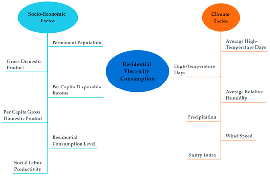
Figure 5.
The corresponding graph of the multidimensional factor index.
In order to deeply understand the influence of various factors on the residential electricity consumption in Beijing and simplify the data, this paper adopts the Spearman rank correlation method to analyze the correlation degree between various indicators and the residential electricity consumption. The formula is shown as Equation (6). The results of the correlation analysis are shown in Table 1.

Table 1.
Spearman rank correlation.
Through, in the socio-economic dimension, between the GDP and the PGDP, there is a high correlation between GDP and residential electricity consumption, so the GDP is selected. Among the remaining four indicators, permanent population and per capita disposable income have the highest correlation. For climate factors, the correlation of average high-temperature days, average relative humidity, and sultry index on residential electricity consumption is relatively high. Therefore, the final six indicators and the scatter diagram of residential electricity consumption in Beijing are shown in Figure 6.
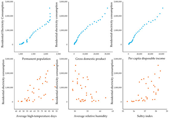
Figure 6.
Scatter plots of selected indicators and residential electricity consumption. Source: National Greenhouse Data.
4.3. Principal Component Analysis under Multiple Indicators: Data Dimensionality Reduction Processing
The names of the variables corresponding to the multi-dimensional indicators are shown in Table 2.
Table 2.
The actual indicator corresponding to the variable.
4.3.1. Raw Data Preprocessing: Standardization and KMO Test
The value of the KMO test is 0.731, as shown in Table 3. It indicates that there is strong collinearity among all variables, which conforms to the condition of principal component analysis. The purpose of the Bartlett test is to determine whether the data is a population with multivariate normal distribution. If the F value of the difference test is significant, it implies that the data subjects to a normal distribution, and further analysis can be conducted. In Table 3, the significance value is equal to 0, which indicates that the data conforms to a normal distribution.
Table 3.
The Kaiser-Meyer-Olkin (KMO) test and the Bartlett’s test.
4.3.2. Data Dimension Reduction: Principal Component Extraction
The principal component analysis is used to extract the principal components from the standardized data, whose results are shown in Table 4.
Table 4.
The principal component extraction results.
From the Table 4, as long as the fourth principal component is calculated, and the cumulative variance contribution rate reaches 99.18%, greater than 85%, therefore, the selection of the top four principal components for subsequent calculation can ensure the integrity of the data when reducing the dimensionality.
The component matrix is shown in Table 5. The matrix that corresponds to the top four principal components is calculated in the subsequent calculation.
Table 5.
Component matrix.
Through Table 4, the eigenvalues are 4.098, 0.803, 0.624, and 0.426, respectively. Multiply the extracted component matrix with the eigenvalue matrix, which obtains , and :
4.4. PCA-MCA—Beijing
After the data are processed by principal component analysis, now, it is suitable for multivariate regression analysis to discuss the linear or nonlinear relationship between multiple variables, then establish the multi-dimensional residential electricity consumption function. The multiple linear regression model established by zy and , ,, is shown in Table 6. The multiple coefficient of determination (R square) is 0.985, indicating a good fitting degree of the regression equation. When the significance is equal to 0.05, the corresponding statistic F is not in the rejection region, indicating that the regression equation is significant.
Table 6.
Multivariate linear regression model.
The coefficient matrix of the multiple linear regression model established above is shown in Table 7, and the four independent variables are all remarkable.
Table 7.
The coefficient matrix of a multiple linear regression model.
The function of calculating variables in SPSS is used to get the relationship between the standardized variable, the dependent variable, and the independent variables, as shown in Equation (11):
The regression equation is reduced by using Equations (3) and (4), and the final expression is shown in Equation (12):
4.5. Results Analysis
4.5.1. Analysis of Factors Affecting Multiple External Disturbances in Residential Electricity Consumption
Without dimensional influence, the sensitivity of indicators in the socio-economic factors and the climate factors is shown in Figure 7.
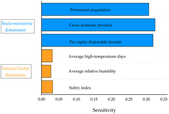
Figure 7.
Sensitivity degree of each index.
In general, Beijing residential electricity consumption is much more sensitive to the socio-economic factors than the climate factors. When the indicators of both dimensions change per unit at the same time, the indicators of the socio-economic dimension change in residential electricity consumption ten times that of the dimension of climate indicators. This is consistent with the results of Spearman’s correlation analysis in Section 4.2. The correlation between socioeconomic factors and residential electricity consumption is generally greater than that of climate factors. Comparing the true data of Beijing with the multi-dimensional measurement model data of residential electricity consumption, the comparison results are shown in Figure 8. The yellow part of the figure shows the error between the true value and the model value.
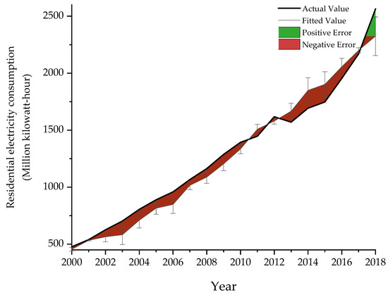
Figure 8.
Comparison between the true and model values of residential electricity consumption in Beijing, China, from 2000 to 2018.
Around 1980, a large-scale warm winter began to appear in China, and the increase of meteorological indexes in this interval was abnormal, which was relatively obvious in North China [51]. Therefore, the influence of abnormal indexes on the fitting degree of the model was relatively large. Except for this period, the average error rate of other years does not exceed 6.6%. Without special circumstances, the fitting degree of the model is quite considerable. Based on the deviation between residential electricity consumption and the true value caused by special circumstances in the current year, such as epidemic of infectious diseases, abnormal climate, demonstrations, etc., this model does not take those into account. Due to the circumstances above, the error of the model still needs to be further studied and improved. The paper uses principal component analysis to reduce its dimensionality due to multiple data dimensions and complex cardinality to facilitate subsequent calculation and analysis, but the data integrity is very high at 99.18%. This shows that the model reduces the data dimension and simplifies the calculation while ensuring the integrity of the original data. The model can be used for reference.
4.5.2. Analysis of the Influence Mechanism of Socio-Economic Factors
The socio-economic factors are highly sensitive to the residential electricity consumption. When the socio-economic indicators change, the residential electricity consumption of Beijing can react quickly to the increase of the indicators. Among three socio-economic indexes studied in this case, gross domestic product has the greatest effect on the residential electricity consumption in Beijing, whose value is 0.325. This index objectively reflects the production development level of Beijing. Moreover, when the gross domestic product of Beijing will increase by 100 million yuan, the electricity consumption will increase by 253,500 kilowatt-hours. The per capita disposable income with a sensitivity of 0.319 directly reflects living standards of people, thus guiding electricity consumption behavior of people. In addition, when the per capita disposable income in Beijing increases by 1 yuan, the residential electricity consumption in Beijing will grow by 125,700 kilowatt-hours. In this dimension, the permanent population with the lowest sensitivity has an agglomerate effect on residential electricity consumption of the whole city. The residential electricity consumption of Beijing increases by 5.2208 million kilowatt-hours while the permanent population of Beijing rises by 10,000. In general, the regional GDP and per capita disposable income have the same mechanism of action on residential electricity consumption, while the agglomeration effect of the permanent population leads to an increase or decrease in residential electricity consumption.
In terms of the correlation degree, the internal indicators of the socio-economic dimension are highly related, which indicates that the degree of collinearity is high. In Beijing, the change of GDP, per capita disposable income, and resident population are shown in Figure 9. It is easy to find that the three indexes have a tendency to grow slowly or even enter into the bottleneck period, which implies that the uncertainty of the socio-economic dimension is declining in the future and gradually, the impact of it becomes stable. In addition, the collinearity is high in the socio-economic dimension. It indicates that the socio-economic indicators will be more predictable.
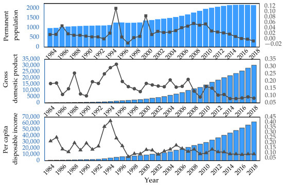
Figure 9.
Changes in socio-economic dimension indicators. Source: Beijing Municipal Bureau of Statistics.
4.5.3. Analysis of the Influence Mechanism of Climate Factors
In the case of the dimension of the climate factors, there is no obvious difference in the mechanism of the three indexes, and all show that rising temperature leads to the increase of sensible temperature and average relative humidity, and then guide the behavior on the demand side. Among the three indexes in the natural dimension, the residential electricity consumption of Beijing is the most sensitive to the sultry index, which can more directly determine whether to use cooling appliances on the demand side. Moreover, the residential electricity consumption of Beijing increases by 287,289,900 kilowatt-hours, while the sultry index rises per unit. The average high-temperature days with a sensitivity of 0.031 directly reflect the days in a year when the average daily temperature exceeds 20 °C. As shown in Figure 10, when the average daily temperature in Beijing exceeds 20 °C, the electricity consumption will reach the turning point and start to rise up. Moreover, when the average-temperature days increase by per unit day, the residential electricity consumption of Beijing will increase by 16,783,400 kilowatt-hours. It can be seen in Equation (11) that the average relative humidity is inverse to the residential electricity consumption in Beijing, which signifies that when the average relative humidity rises, the residential electricity consumption decreases. Climate change is a very complex process. In Beijing, climate change leads to an increase in evaporation and then a decrease in average relative humidity. When the average relative humidity [52] decreases by 1%, residential electricity consumption increases by 62,761,500 kilowatt-hours.
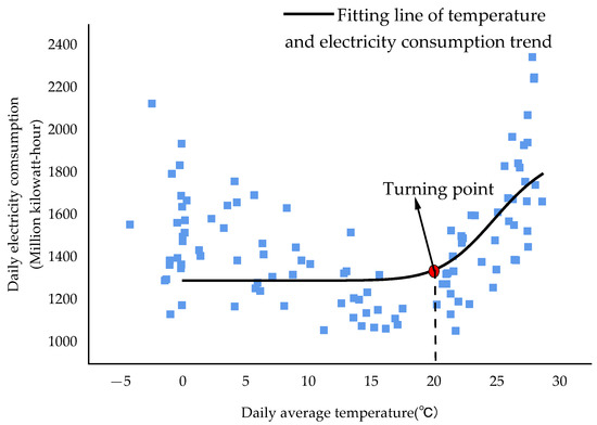
Figure 10.
The relationship between daily average temperature and daily electricity consumption in Beijing, China.
In terms of the correlation degree, among climate indicators, the degree of collinearity of each index is small, which implies that the difference of each index is obvious. Therefore, it is impossible to simplify multiple indicators into the same indicator for forecasting, which makes the forecasting work more difficult. In addition, with the aggravation of climate change and frequent occurrence of extreme weather, the uncertainty of each indicator increases, which means that the impact in the climate dimension on residential electricity consumption is abrupt. Therefore, it is particularly important to conduct individual research on each indicator and accurately predict the impact of climate factors on residential electricity consumption.
5. Conclusions and Optimal Strategies Based on the Case Study
5.1. Conclusions
(1) The PCA-MCA multi-factor measurement model has high data integrity and low error rate.
The multi-dimensional residential electricity consumption model was constructed through the principal component analysis to data dimension reduction process, which simplified the calculation and guaranteed the data integrity of 99.18% at the same time. Using the actual data for historical inspection and operation of the model, the results showed that under the condition of no abnormal circumstances, the simulated value of the output variable is within ±7% of the actual value. It belongs to the credible scope. The reliability of the model is high and can effectively calculate the residential electricity consumption. The growth rate in the latter of the model prediction curve is less than the actual value, which shows that according to the forecast pattern of this article, the growth of residential electricity consumption in Beijing should be slowed down after the socio-economic factors stabilize. However, the actual situation is contrary to the fact that the growth rate of actual residential electricity consumption has increased, which indicates that the abnormal climate factors have played a great role in the growth of residential electricity consumption and disrupted the trend of residential electricity consumption growth. Therefore, it is necessary to pay great attention to the abnormal situation of climate change and formulate some policies to improve the situation.
(2) The influence mechanism of socio-economic factors and climate factors is heterogeneous.
The results of the model show that the socio-economic factor is positively correlated with the residential electricity consumption of Beijing, and the correlation degree of the internal index is close, with a sign of slowing, which is the stable influence. However, the correlation degree of climate indexes is uneven, with both positive and negative degrees. The intensification of climate change leads to the unclear trend of the index change, which is the mutational effect. It indicates that the collinearity degree of the socio-economic factors on the residential electricity consumption of Beijing is much greater than that of climate factors. In general, nowadays, the influence of the socio-economic dimension and the climate dimension on residential electricity consumption has become heterogeneous. The growth of socio-economic indicators has slowed down, or some of them have even entered a bottleneck period, while the internal indicators of climate factors have a small degree of collinearity and the uncertainty caused by the aggravation of climate change has increased. Faced with China’s current rapid growth in residential electricity consumption and intensified climate change, based on the heterogeneity of socio-economic factors and climatic factors, the government can adopt appropriate control and measurement measures for different factors.
Based on principal component analysis and multiple linear regression, this research constructed a multi-factor residential electricity consumption model, and quantitative analysis was carried out through this model. At the same time, this paper performed a case study of Beijing and discussed and selected the multi-factor indicators that highly related to the residential electricity consumption. On the basis outlined above, the multi-factor residential electricity consumption function of Beijing was constructed, which was used to analyze the different influence mechanisms of the two factors on residential electricity consumption. Ultimately, the optimal strategies were provided for ensuring the stable operation of the regional power system. The research results effectively solved the visual measurement of the external dimensions of residential electricity consumption in Beijing and expanded the heterogeneous understanding of the influence mechanisms of different factors. Some optimization strategies were provided to manage power demand side effectively, which are beneficial to the sustainable development of the regional power industry.
5.2. Optimal Strategies
The case study of Beijing shows that the residential electricity consumption is affected by two factors, which begin to become heterogeneous. In view of how to strengthen the power demand side management in order to better realize the optimal allocation of resources, the following three strategies are proposed.
5.2.1. Actively Promote the Reform of a New Type of Electricity Pricing Policy and Guide Residents to Cut Peak Load from the Demand Side
In the socio-economic aspects, the per capita disposable income is highly sensitive to the residential electricity consumption in Beijing. The situation of Beijing shows that residential load gradually diversifies along with the development of the economy, which means that the supply side has more difficulty accurately predicting residential electricity consumption. Therefore, adjusting the peak load from the demand side becomes extremely important. One paper showed that the real-time pricing strategy of user electrical appliance classification can achieve the effect of peak load cutting better than the peak and valley price currently implemented. Moreover, the real-time pricing model is not only time-effective but also maximizes the utility of both the supplier and the demander [53]. By implementing the real-time electricity price strategy of user electrical appliances classification, the government could indirectly influence the residential electricity consumption level, which feeds back the change of total residential electricity consumption. Finally, it plays a role in the stabilization of residential load. While meeting the same utility, it reduces power consumption and power demand, which meets the requirements of regional power sustainable development.
5.2.2. Strengthen the Forecasting Accuracy of Diversified Loads and Ensure the Stability Load Running within the Plan
From the analysis in this paper, it could be seen that the socio-economic indicators of Beijing have a high degree of collinearity. There are gradually slowing down and even entering the bottleneck period. It indicates that the socio-economic indicators tend to be stable, accurate, and predictable. Besides, with the construction of a smart power grid, the renovation of smart electric equipment on residents of Beijing is being implemented. Real-time monitoring equipment such as smart electricity meters, smart sockets, and big data sharing platform are constantly improved. What is mentioned above makes the collection of residential information more complete on the supply side, which lays a foundation for the accurate prediction of residential electricity consumption. The government should combine with the big data platform to accurately predict the trend of socio-economic indicators and measure the residential electricity consumption under the stable influence. It can ensure that electricity consumption of this part is carried out within the plan and can make the optimal allocation of grid resources.
5.2.3. Use Small-Scale Renewable Energy-Generating Units to Respond to the Sudden Load Caused by Climate Change
According to the model results, the climate indicators are of great uncertainty and vary in correlation degrees, which have a mutational impact on the residential electricity consumption. Therefore, it is very important to eliminate the impact of the mutational load on the stability of the power system. The government should encourage local departments to take measures according to local conditions. Moreover, it can use renewable energy and energy storage technology to set up small-scale renewable energy-generating units in different areas, such as photovoltaic power generation and wind power generation. With those, we can cope with the small-scale power consumption peak caused by the uncertainty of climate indicators, thereby alleviating the pressure of sudden load on power demand. This will not only ensure the stable operation of the load under the abrupt power consumption peak, but also realize the incremental substitution of clean energy, and gradually solve the current contradiction in the consumption of renewable energy in power demand side management of China.
Author Contributions
Data curation, J.L. and D.W.; Formal analysis, Y.S.; Investigation, X.S.; Methodology, Y.S. and D.W.; Software, D.W.; Supervision, J.L. and X.S.; Writing—original draft, Y.S. and J.L.; Writing—review & editing, Y.S., J.L., D.W. and X.S. All authors have read and agreed to the published version of the manuscript.
Funding
This research is supported by the National Natural Science Foundation of China (NSFC) (72074074).
Informed Consent Statement
Not applicable.
Data Availability Statement
Publicly available datasets were analyzed in this study. This data can be found here: [https://www.climate.gov, http://www.cma.gov.cn/, http://www.stats.gov.cn/, http://tjj.beijing.gov.cn/, http://data.sheshiyuanyi.com/WeatherData/] accessed on 15 February 2021.
Conflicts of Interest
The authors declare no conflict of interest.
References
- Holtedahl, P.; Joutz, F.L. Residential electricity demand in Taiwan. Energy Econ. 2004, 26, 201–224. [Google Scholar] [CrossRef]
- Jennen, M.; Verwijmeren, P. Agglomeration Effects and Financial Performance. Urban. Stud. 2007, 47, 2683–2703. [Google Scholar] [CrossRef]
- Zhu, X.; Li, L.; Zhou, K.; Zhang, X.; Yang, S. A meta-analysis on the price elasticity and income elasticity of residential electricity demand. J. Clean. Prod. 2018, 201, 169–177. [Google Scholar] [CrossRef]
- Liang, L.; Wu, W.; Rattan, L.; Guo, Y.B. Structural change and carbon emission of rural household energy consumption in Huantai, northern China. Renew. Sustain. Energy Rev. 2013, 28, 767–776. [Google Scholar] [CrossRef]
- Dalir, F.; Shafie-Pour-Motlagh, M.; Ashrafi, K. Sensitivity analysis of parameters affecting carbon footprint of fossil fuel power plants based on life cycle assessment scenarios. Glob. J. Environ. Sci. Manag. 2016, 3, 75–88. [Google Scholar]
- Koppe, A. Regulate, Reuse, Recycle: Repurposing the Clean Air Act to Limit Power Plants’ Carbon Emissions. Ecol. Law Q. 2014, 41, 349–376. [Google Scholar]
- Lin, W.; Chen, B.; Luo, S.; Liang, L. Factor Analysis of Residential Energy Consumption at the Provincial Level in China. Sustainability 2014, 6, 7710–7724. [Google Scholar] [CrossRef]
- Felimban, A.; Prieto, A.; Knaack, U.; Klein, T.; Qaffas, Y. Assessment of Current Energy Consumption in Residential Buildings in Jeddah, Saudi Arabia. Buildings 2019, 9, 163. [Google Scholar] [CrossRef]
- Zhou, X.Q. Development history, planning and implementation of “West-to-East Power Transmission” in my country. Power Syst. Technol. 2003, 27, 1–5. [Google Scholar]
- Fu, H.H.; Cai, G.T.; Zhao, D.Q. The Temporal-Spatial Evolution of the Southern Corridor of West-to-East Power Transmission Project in China. Appl. Mech. Mater. 2014, 521, 485–489. [Google Scholar] [CrossRef]
- McLoughlin, F.; Duffy, A.; Conlon, M. Characterising domestic electricity consumption patterns by dwelling and occupant socio-economic variables: An Irish case study. Energy Build. 2011, 43, 240–248. [Google Scholar] [CrossRef]
- Zhou, S.; Teng, F. Estimation of urban residential electricity demand in China using household survey data. Energy Policy 2013, 61, 394–402. [Google Scholar] [CrossRef]
- Nawaz, S.; Iqbal, N.; Anwar, S. Modelling electricity demand using the STAR (Smooth Transition Auto-Regressive) model in Pakistan. Energy 2014, 78, 535–542. [Google Scholar]
- Al Irsyad, M.; Nepal, R.; Halog, A. Exploring drivers of sectoral electricity demand in Indonesia. Energy Sources Part B Econ. Plan. Policy 2018, 13, 9–10. [Google Scholar] [CrossRef]
- Amusa, H.; Amusa, K.; Mabugu, R. Aggregate demand for electricity in South Africa: An analysis using the bounds testing approach to cointegration. Energy Policy 2009, 37, 4167–4175. [Google Scholar] [CrossRef]
- Shibano, K.; Mogi, G. Electricity consumption forecast model using household income: Case study in Tanzania. Energies 2020, 13, 2497. [Google Scholar] [CrossRef]
- Aydin, E.; Brounen, D. The impact of policy on residential energy consumption. Energy 2019, 169, 115–129. [Google Scholar] [CrossRef]
- Jo, H.H.; Jang, M.; Kim, J. How Population Age Distribution Affects Future Electricity Demand in Korea: Applying Population Polynomial Function. Energies 2020, 13, 5360. [Google Scholar] [CrossRef]
- Anna, A.; Giuseppe, P.; Chang, S.; Jacopo, T. Hot weather and residential hourly electricity demand in Italy. Energy 2019, 177, 44–56. [Google Scholar]
- Allen, M.R.; Fernandez, S.J.; Fu, J.S.; Olama, M.M. Impacts of climate change on sub-regional electricity demand and distribution in the southern United States. Nat. Energy 2016, 1, 16103. [Google Scholar] [CrossRef]
- Auffhammer, M.; Baylis, P.; Hausman, C.H. Climate change is projected to have severe impacts on the frequency and intensity of peak electricity demand across the United States. Proc. Natl. Acad. Sci. USA 2017, 114, 1886–1891. [Google Scholar] [CrossRef] [PubMed]
- Shourav, M.S.A.; Shahid, S.; Singh, B.; Mohsenipour, M.; Chung, E.S.; Wang, X.J. Potential Impact of Climate Change on Residential Energy Consumption in Dhaka City. Environ. Model. Assess. 2018, 23, 131–140. [Google Scholar] [CrossRef]
- Franco, G.; Sanstad, A.H. Climate change and electricity demand in California. Clim. Chang. 2008, 87, 139–151. [Google Scholar] [CrossRef]
- Jo, S.W.; Park, R.J.; Kim, K.H.; Kwon, B.S.; Park, H.S. Sensitivity analysis of temperature on special day electricity demand in Jeju Island. Trans. Korean Inst. Electr. Eng. 2018, 67, 1019–1023. [Google Scholar]
- Mukhopadhyay, S.; Nateghi, R. Climate sensitivity of end-use electricity consumption in the built environment: An application to the state of Florida, United States. Energy 2017, 128, 688–700. [Google Scholar]
- Fumo, N.; Biswas, M.R. Regression analysis for prediction of residential energy consumption. Renew. Sustain. Energy Rev. 2015, 47, 332–343. [Google Scholar] [CrossRef]
- Wang, H.W.; Huang, Y.S.; Jiang, Y.Q.; Liu, S.J. Medium—And long-term probabilistic prediction of household electricity consumption based on Lasso algorithm and Gaussian process regression. J. North. China Electr. Power Univ. (Nat. Sci. Ed.) 2019, 46, 27–35. [Google Scholar]
- Yang, Z.M.; Li, W.R.; Yan, Z.M. Relationship between temperature change and power demand—Empirical evidence based on Panel data of Chinese cities from 2000 to 2014. J. Beijing Inst. Technol. (Soc. Sci.) 2019, 21, 44–55. [Google Scholar]
- Blazquez, L.; Filippini, M.; Boogen, N. Residential electricity demand in Spain: New empirical evidence using aggregate data. Energy Econ. 2013, 36, 648–665. [Google Scholar] [CrossRef]
- Shahzad, A.; Zafar, M.; Naeem, N.S.M. Dilemma of direct rebound effect and climate change on residential electricity consumption in Pakistan. Energy Rep. 2018, 4, 323–327. [Google Scholar]
- Zheng, S.; Huang, G.; Zhou, X.; Zhu, X. Climate-change impacts on electricity demands at a metropolitan scale: A case study of Guangzhou, China. Appl. Energy 2020, 261, 114295. [Google Scholar] [CrossRef]
- Liu, C.; Sun, B.; Zhang, C.; Li, F. A hybrid prediction model for residential electricity consumption using holt-winters and extreme learning machine. Appl. Energy 2020, 275, 115383. [Google Scholar] [CrossRef]
- Hussain, A.; Maha, A. Residential electricity consumption in the state of Kuwait. Environ. Pollut. Clim. Chang. 2018, 2, 153. [Google Scholar]
- Elkamel, M.; Schleider, L.; Pasiliao, E.L.; Diabat, A.; Zheng, Q.P. Long-term electricity demand prediction via socioeconomic factors a machine learning approach with Florida as a case study. Energies 2020, 13, 3996. [Google Scholar] [CrossRef]
- Khan, Z.; Ullah, A.; Ullah, W. Electrical Energy Prediction in Residential Buildings for Short-Term Horizons Using Hybrid Deep Learning Strategy. Appl. Sci. 2020, 10, 8634. [Google Scholar] [CrossRef]
- Ngabesong, R.; Mclauchlan, L. Implementing “R” Programming for Time Series Analysis and Forecasting of Electricity Demand for Texas. In Proceedings of the 2019 IEEE Green Technologies Conference (GreenTech), Lafayette, LA, USA, 3–5 April 2019. [Google Scholar]
- Saravanan, S.; Kannan, S.; Amosedinakaran, S.; Thangaraj, C. India’s electricity demand estimation using Genetic Algorithm. In Proceedings of the 2014 International Conference on Circuits, Power and Computing Technologies [ICCPCT-2014], San Francisco, CA, USA, 22–24 October 2014. [Google Scholar]
- Ningpramuda, A.D.; Sarno, R.; Suryani, E.; Fauzan, A.C. Dynamic simulation of electricity supply and demand for industry sector in East Java. In Proceedings of the 2017 3rd International Conference on Science in Information Technology (ICSITech), Bandung, Indonesia, 25–26 October 2017. [Google Scholar]
- Sowiński, J. Forecasting of electricity demand in the region. In Proceedings of the 14th International Scientific Conference “Forecasting in Electric Power Engineering” (PE 2018), Singapore, 22–23 August 2019. [Google Scholar]
- Kartikasari, M.D.; Prayogi, A.R. Demand forecasting of electricity in Indonesia with limited historical data. J. Phys. Conf. Ser. 2018, 1, 974. [Google Scholar] [CrossRef]
- Guefano, S.; Tamba, J.G.; Azong, T.E.; Monkam, L. Forecast of electricity consumption in the Cameroonian residential sector by Grey and vector autoregressive models. Energy 2021, 214, 118791. [Google Scholar] [CrossRef]
- Guo, C.Q.; Chen, X.Z. SPSS implementation of principal Component Regression. Stat. Decis. Mak. 2011, 5, 157–159. [Google Scholar]
- Liao, H.; Liu, Y.N.; Gao, Y.X.; Hao, Y.; Ma, X.; Wang, K. Forecasting residential electricity demand in provincial China. Environ. Sci. Pollut. Res. 2017, 24, 6414–6642. [Google Scholar] [CrossRef] [PubMed]
- Lin, Y.; Wang, J.W.; Zhou, H.Q.; Yi, Y.D.; Jun, P.Y. Frame Construction and Task Analysis of Smart Energy in the Construction of Smart City. Energy Power Eng. 2020, 12, 4. [Google Scholar]
- Leonie, W.; Anders, L.; Maximilian, A. North–south polarization of European electricity consumption under future warming. Proc. Natl. Acad. Sci. USA 2017, 114, 201704339. [Google Scholar]
- Cheng, L.Y.; Feng, Y.H.; Wang, N.; Xu, N.; Luo, W. Load characteristics analysis and peak shaving margin calculation of Beijing-Tianjin and North Hebei power grids. North China Electr. Power Technol. 2015, 11, 56. [Google Scholar]
- Zhang, B.; Shi, P.R.; Jiang, C. Analysis of influence of meteorological factors on summer load characteristics of Beijing-Tianjin-Tangshan power grid. Electr. Power Autom. Equip. 2013, 33, 140–144. [Google Scholar]
- Li, Y.; Pizer, W.A.; Wu, L. Climate change and residential electricity consumption in the Yangtze River Delta, China. Proc. Natl. Acad. Sci. USA 2019, 116, 472–477. [Google Scholar] [CrossRef] [PubMed]
- Maia-Silva, D.; Kumar, R.; Nateghi, R. The critical role of humidity in modeling summer electricity demand across the United States. Nat. Commun. 2020, 11, 1–8. [Google Scholar] [CrossRef] [PubMed]
- Li, C.; Guo, W.L.; Wu, J.; Jin, C.X. BP neural network based on prediction method of daily maximum power load in summer in Beijing. Clim. Environ. Res. 2019, 24, 135–142. [Google Scholar]
- Wei, F.Y.; Cao, H.X.; Wang, L.P. Statistical Facts of China’s climate warming process in the 1980s and 1990s. J. Appl. Meteorol. 2003, 1, 79–86. [Google Scholar]
- Lu, A.G. Impact of global warming on regional relative humidity change in China. Ecol. Environ. 2013, 22, 1378–1380. [Google Scholar]
- Li, J.X.; Zhang, W.C.; Gao, Y. Research on real-time pricing of smart grid based on user electrical appliance classification. China Manag. Sci. 2019, 27, 210–216. [Google Scholar]


Publisher’s Note: MDPI stays neutral with regard to jurisdictional claims in published maps and institutional affiliations. |
© 2021 by the authors. Licensee MDPI, Basel, Switzerland. This article is an open access article distributed under the terms and conditions of the Creative Commons Attribution (CC BY) license (http://creativecommons.org/licenses/by/4.0/).