Abstract
Emergency events can induce serious traffic congestions in a local area which may propagate to the upstream roads, and even the whole network. Until now, the methodology forecasting spatiotemporal boundary propagation of emergency-event-based traffic congestions, with both explicitness and road network availability, has not been found. This study develops a new method for predicting spatiotemporal boundary of the congestion caused by emergency events, which is more applicable and practical than cell transmission model (CTM)-derived methods. This method divides the expressway network into different sections based on their functions and the shockwave direction caused by the emergency events. It characterizes the velocity of the moving congestion boundary based on kinetic wave theory and volume–density relationship. After determining whether the congestion will spread into the network level through an interchange using a new concept, highway node acceptance capacity (HNAC), we can predict the spatiotemporal boundary and corresponding traffic condition within the boundary. The proposed method is tested under four traffic incident cases with corresponding traffic data collected through field observations. We also compare its prediction performances with other methods used in the literature.
1. Introduction
Emergency events such as traffic accidents are disruptive to traffic flow. When an emergency event happens, it can induce serious traffic congestion in the road section, and it can further spread to upstream road network. Predicting the evolution of the traffic congestion (i.e., the spatiotemporal boundary of traffic congestion), also the traffic condition in the congested area is critical to design effective measures to address the negative effects of these events. For instance, the traffic managers could close some entrances and diverge the trapped vehicles according to the predicted spatiotemporal boundary to reduce the traffic congestion.
The spatiotemporal boundary of emergency-event-based traffic congestions is defined as the interface of traffic wave caused by an incident [1]. Related studies proposed different methodologies to determine the spatiotemporal boundary of traffic congestions, including kinetic wave theory [2,3,4], cell transmission model (CTM), etc. [5,6,7,8,9]. Further, methods are also proposed for estimating queue length [10,11,12,13,14] and measuring traffic flow dynamics [15,16,17,18,19]. Kinetic wave theory could provide the explicit value of spatiotemporal boundary moving velocity caused by emergency event, but it is not suitable in road network because it does not provide a way to analyze congestion propagation in interchanges. Some CTM-based models can solve the problem of congestion propagation in interchange [7,8,9,20,21,22], but these works did not provide results in forms of clear values or explicit equations, which were not applicable enough. Till now, the methodology on spatiotemporal boundary of emergency-event-based traffic congestions, with both explicitness and road network availability, has not been found.
In an interchange area, the traffic volume that can merge into the targeted expressway from the intersected expressway connected by a ramp is typically limited. We define the maximum merging traffic volume as the highway node acceptance capacity (HNAC) [23]. In a real driving environment, if the traffic volume merging into an expressway exceeds the HNAC of the targeted road section (i.e., the expressway where the flow will merge into), dramatic traffic oscillations and serious traffic congestion will be formed in the merging ramp. In this study, HNAC will be used as a key element in predicting the spatiotemporal boundary of the congestion caused by emergency events in an expressway network. The reasons are as follows. We can explicitly evaluate whether the congestion will propagate from the targeted expressway to the intersected expressway by just looking into HNAC. Besides, HNAC can be explicitly computed by leveraging traffic flow parameters which could be directly obtained from roadside monitoring facilities, or historically recorded (e.g., traffic volume, ratio of heavy vehicle). Thereby, an HNAC-based prediction method is more applicable and practical for characterizing the spatiotemporal boundary of the congestion in an expressway network.
In this study, Section 2 provides a literature review on analyzing a traffic congestion spatiotemporal boundary. Section 3 depicts the expressway network subdivision method considering road section functions and the shockwave direction caused by the emergency events (Section 3.1). Moreover, two procedures including kinetic wave theory integrating volume–density relationship (Section 3.2) and HNAC (Section 3.3) are detailed and constructed. In Section 4 and Section 5, we test the proposed method under four traffic incident cases and compare its prediction performances with other methods used in the literature. The accuracy and practicality of the proposed method is proved.
2. Related Studies on a Traffic Congestion Spatiotemporal Boundary
To forecast the spatiotemporal boundary of traffic congestion, two sorts of methods were usually adopted: kinetic wave theory incorporating traffic fundamental diagram [10,11,12,13,14,24,25,26] and CTM-based models [7,8,9,20,21,22].
Kinetic wave theory, also known as LWR theory [27,28], is a good tool for characterizing macroscopic traffic dynamics. It can well describe the traffic waves (e.g., wave velocity) and is widely studied and used in the literature. However, evaluating a traffic congestion spatiotemporal boundary in a road section only using classical LWR theory may not be sufficient [2,3,4]. To obtain the spatiotemporal boundary moving velocity (traffic wave velocity), the traffic fundamental diagram is also needed [29,30,31,32,33,34,35,36]. By applying kinetic wave theory incorporating traffic fundamental diagram, the explicit value of spatiotemporal boundary moving velocity caused by emergency events could be calculated in a relatively simple way: input the initial traffic volume and density. Furthermore, in using this method, real-time traffic condition (volume, density, velocity) in congested road sections could also be obtained [15,16,17,18,19]. It should be noted that this sort of method has some shortages. First, this method was usually adopted to analyze a traffic congestion spatiotemporal boundary in a road segment, studies on large-scale networks were limited. This is because the judgement of whether the spatiotemporal boundary will spread into an intersected road through an interchange could not be easily and accurately answered [23]. Although some research focus on network were found [16], most of these models were developed and calibrated using simulations or unrealistic assumptions; large-scale field data depicting real-time traffic flows are needed. Second, most of these studies do not consider the impacts of heavy vehicles in the flow and heterogeneous traffic volumes in different lanes.
The other sort of method is CTM-based models [5,6,7,9,20,21,22], which is also extensively used for modeling traffic congestion spatiotemporal boundaries, especially in road network. In CTM, road network is divided into small cells based on its function or geometric form, following Daganzo’s early work [7]. For example, an interchange can be represented by merge cells and diverge cells based on traffic flow direction. Merge cells consist of two entering links and one leaving link. Diverge cells consist of one entering link and two leaving links. The traffic flow in one cell is assumed to be homogeneous. Following this routine, CTM-based models could analyze the spatiotemporal boundary of traffic congestion in a road network. However, CTM-based models have two shortages in solving emergency-event-based traffic congestions. First, compared to kinetic wave related ideas, the CTM ideas are relatively complex, lacking some clarity in calculation, and showing some difficulties in putting them into practice. For example, in Sakakibara’s work [7] and Meng’s work [21], we could not explicitly answer whether a congestion will spread to intersected road sections in an interchange by using parameters which could be observed using roadside monitoring facilities, or historically recorded. Second, CTM-based methods are hard to reflect traffic congestion spatiotemporal boundary moving direction in emergency events. For instance, if an emergency event happened downstream an interchange, the congestion would spread to an intersected road through a merging ramp, and the diversion ramp could be omitted.
In summary, on one hand, the kinetic wave theory integrating with an appropriate volume–density relationship model can better characterize spatiotemporal boundary propagation in expressway sections in an explicit way [37,38,39,40]. On the other hand, CTM-based methods show advantages to discriminate traffic flow characters in different road sections in a network. However, these two models have not been integrated to predict spatiotemporal boundary propagation of emergency-event-based congestion in expressway networks. That is because the current literature cannot accurately evaluate whether the congestion (spatiotemporal boundary) will spread into the intersected expressway sections through interchanges. This problem is well addressed by HNAC defined in our previous work [23]. Following that, this study proposes a method which integrates kinetic wave theory, volume–density model and CTM to predict the spatiotemporal boundary of emergency-event-based traffic congestion propagation in expressway networks. Applications using field data found that the proposed method can accurately predict the evolution of traffic congestion and corresponding traffic conditions.
3. Methodology
3.1. Dividing Expressway Network
An expressway network contains basic road sections (BRSs) and interchanges. For BRSs, it is defined as the section between the merging section (ME) and the diversion section (DI) of two adjacent interchanges. For an interchange, the CTM methods divide it into merging cell and diversion cell following the classical work by Carlos F. Daganzo [5,6,7,8,9,20,21,22], as depicted in Section 2. The CTM method seeks to characterize the traffic flow using the direction of vehicle movement. However, in emergency events, traffic congestion propagation direction is converse from traffic flow in BRSs. Moreover, the diversion ramp in interchange will not be affected by emergency-event-based traffic congestion, shown in Figure 1. According to abovementioned two phenomena, an expressway network could be subdivided as shown in Figure 1 in emergency events, which is different from CTM methods.
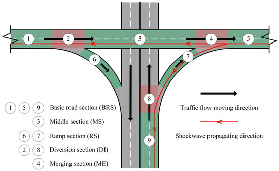
Figure 1.
Expressway network subdivision method considering emergency-event-based traffic congestion propagation particularity.
In Figure 1, the emergency event is assumed to happen in downstream section 5 (BRS), and red arrow represents the spreading direction of traffic congestion spatiotemporal boundary. In CTM methods, sections 1, 2, 3, and 6 belong to the diversion area while sections 3, 4, 5, and 7 belong to the merging area. It should be noted that sections 1, 2, 3, 4 and 5 are treated as cells while sections 6 and 7 are treated as links. That is to say, ramp length is neglected. However, in real expressway network, ramp length can be as large as 1 km. In cases of emergencies, the velocity of both traffic flow and spatiotemporal boundary propagation is low [41]. The time spent in the ramp section should not be ignored. Therefore, in this section, ramp sections (RSs) are treated as a special BRS controlled by lower bound of velocity. Besides, in CTM methods, diversion section (DI) 2 and section 1 are integrated into one cell, so the same of merging section (ME) and section 5. Considering the traffic operation characters in DI and section 1 (also in ME and section 5), integrating them into one cell is not quite appropriate. To be more specific, lane-changing behaviors in DI and ME can more easily lead a bottleneck compared to the traffic flow in BRSs. According to abovementioned traffic characters in DI and ME, and combing their short length, they are treated as junctions in the subdivision method. Moreover, the area between DI and ME is named as the middle section (MS). The traffic flow character in MSs is similar to BRSs, but their length is generally smaller than BRSs’. When an emergency event happens in downstream section 5, spatiotemporal boundary propagation direction is depicted by red arrow in Figure 1. Obviously, spatiotemporal boundary will propagate in two directions; the first is along the route involving sections 5, 4, 3, 2, 1, and the second is uptracking to section 9 through ramp 7. Therefore, practically, Section 6 will not be included in the expressway network of this study.
3.2. Kinetic Wave and Volume–Density Relationship Model
Traffic congestion spatiotemporal boundary propagation can be interpreted as kinetic wave spreading (or shockwave). The phenomenon is similar to the kinetic wave caused by capacity collapse, creating serious and wide-spread traffic congestion. As is shown in Figure 2, to model the kinetic wave propagation, the traffic conditions before the emergency event in each section of the expressway network are needed.
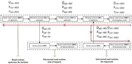
Figure 2.
Background traffic condition of expressway network in emergency events.
Following spatiotemporal boundary propagation and traffic moving direction in Figure 2, propagation velocity should be computed in the following five sections: BRSs of the emergency event, MS upstream from the emergency event, BRSs upstream from the emergency event, merging RSs, and BRSs intersected (see Figure 1). Denote , , and as the traffic condition at the emergency event location. According to kinetic wave theory [2,3,4,27,28], spatiotemporal boundary propagation velocity in emergency-event BRSs could be obtained using Equation (1). Moreover, and could be estimated through capacity loss in the Highway Capacity Manual [42]. When the congestion covers emergency-event BRSs, traffic condition in this section will be the same as that in the emergency event position. The spatiotemporal boundary propagation velocity in MS upstream from the emergency event could be calculated using Equation (2). Note that in Equation (2), . When the spatiotemporal boundary passed, we had a new traffic condition , , and . Thus, spatiotemporal boundary propagation velocity in BRSs upstream from the emergency event could be computed by Equation (3). In emergency events, when congestion forms in emergency-event BRSs, there will not be enough spaces for on-ramp vehicles to merge, and traffic in RSs would be blocked. Setting the block density of merging RSs as , spatiotemporal boundary propagation velocity could be obtained using Equation (4). When merging RSs become blocked, on-ramp vehicles in intersected BRSs have to stop in the right-side lane and keep waiting, causing a bottleneck. Setting traffic condition in a bottleneck as and , then spatiotemporal boundary propagation velocity in intersected BRSs can be estimated using Equation (5).
Note that the relationship between traffic volume and density is unknown. The appropriate volume–density relationship model is needed as depicted in Section 2. In this study, a general logistic-based volume–density model proposed in our previous work [41] is adopted. We use this model because it can well describe the traffic flow characters in heavy vehicle mixed situation. Unlike Western developed countries, the dynamic performance of heavy vehicles in China is generally lower, and overload occurs very often, leading to large velocity gaps, compared to passenger vehicles. This phenomenon makes traffic flow instable, especially in high heavy vehicle proportion [41,43,44,45,46,47,48,49].
This logistic-based model is described in Equations (6)–(8). Equation (6) represents the relationship between traffic volume and traffic density , considering heavy vehicle mixing ratio . In this equation, parameters , and are used. Among them, represents free flow velocity, represents the traffic density when the traffic flow becomes blocked (block density), and represents the traffic density when traffic saturation (V/C) reaches 1 (transitional density). Moreover, there are two variable indicators and , which could be calculated using Equations (7) and (8), respectively.
3.3. HNAC-Based Boundary Condition
As introduced in Section 1, HNAC represents the maximum merging traffic volume from intersected expressway to targeted expressway in an interchange, through the merging ramp [23]. To be more specific, combining the contents in Figure 1 and Figure 2, when traffic flow in emergency-event BRSs is moving slowly (notice, not blocked), it still has the ability to receive some merging volume. The explicit number of maximum merging volume is HNAC. If actual merging volume was bigger than HNAC, traffic flow in merging RSs would be blocked and would further impact the traffic in intersected BRSs. The advantage of HNAC is that it provides an explicit threshold, which was not found in related studies [7,8,9,20,21,22], as mentioned in Section 1. According to HNAC, traffic management agencies can make direct judgement as to whether an emergency-event-based congestion will spread into intersected expressway. This advantage makes HNAC more practical. HNAC could be calculated using Equations (9)–(11). In these equations, is the traffic volume in emergency-event BRSs, as introduced in Section 3.2. Two variable indicators and could be calculated using heavy vehicle mixing ratio of traffic flow in emergency-event BRSs . Additionally, and could be directly observed using roadside monitoring facilities.
Moreover, even in the most serious emergency events, spatiotemporal boundary propagation is not endless. Therefore, some propagation boundary conditions should be found. In previous parts, spatiotemporal boundary propagation is regarded as kinetic-wave delivered. When value of propagation velocity is negative, spatiotemporal boundary propagation will continue uptracking. When value of propagation velocity is positive, spatiotemporal boundary propagation will stop uptracking. Furthermore, in BRSs, MS and RSs, the coming traffic flow remains stable; the boundary only exists in DI, where the traffic load could be lightened by the diversion. Therefore, the boundary conditions of DI upstream and intersected can be described as
3.4. Procedure of Forecasting Spatiotemporal Boundary Propagation in Expressway Network
Summarizing all the contents introduced above, an HNAC, kinetic wave theory and general logistic volume–density model-based, systematic and explicit procedure forecasting spatiotemporal boundary propagation in expressway networks is built, shown in Figure 3. The following steps describe how to apply this procedure to forecast spatiotemporal boundary propagation in expressway networks:
Step 1. Inputting emergency event capacity loss and traffic condition of emergency event BRS, obtaining propagation time T-EM-BRS using Equation (1).
Step 2. Making judgement of whether spatiotemporal boundary will uptrack in merging RSs using Equation (9). The spatiotemporal boundary will not uptrack in merging RSs, neglecting intersected BRSs.
Step 3. If yes (the spatiotemporal boundary will uptrack in merging RSs) in step 2, then compute the spatiotemporal boundary propagation velocity using Equation (4), making uptrack judgement in intersected DI using Equation (13). If no (the spatiotemporal boundary will not uptrack in DI intersected), then output the propagation time in merging RS T-UP-RS, and neglect the intersected BRS. If yes (the spatiotemporal boundary will uptrack in DI intersected), then onto step 4.
Step 4. If yes (the spatiotemporal boundary will uptrack in DI intersected) in step 3, then execute cyclic calculation in intersected sections till the boundary conditions are satisfied, and output the whole propagation time in intersected sections T-INTERSECTED.
Step 5. This step is in the same position as step 3; whatever the judgement of step 2 is, this step will continue. In this step, calculate spatiotemporal boundary propagation velocity using Equation (2).
Step 6. In this step, make uptrack judgement in upstream DI using Equation (12). If no (the spatiotemporal boundary will not uptrack in upstream DI), output propagation time in upstream WS T-UP-MS, and neglect upstream BRSs. If yes (the spatiotemporal boundary will uptrack in upstream DI), then onto step 7.
Step 7. If yes (the spatiotemporal boundary will uptrack in upstream DI) in step 6, carry out cyclic calculation in upstream sections until the boundary conditions are satisfied, and output whole propagation time in upstream sections T-UPSTREAM.
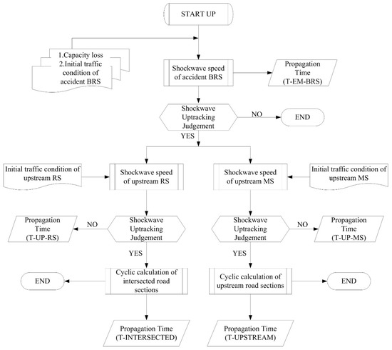
Figure 3.
Procedure forecasting spatiotemporal boundary propagation in expressway network in emergent situations.
4. Cases of Spatiotemporal Boundary Propagation in Expressway Network in Emergent Situations
A case study is used to test the effectiveness of the proposed HNAC-based method built in Section 3. We consider four traffic incident cases (TIC) in the Ring Expressway (G3001) of Xi’an, China. The incidents information is historically recorded by the traffic management department. Traffic data, including real-time cross-section data and historical data, corresponding to each incident, are collected through roadside monitoring facilities. These incident cases all cause large capacity loss and wide-spread congestion. Further, the number of closed lanes remains unchanged before the incident is removed. Therefore, the spatiotemporal boundary propagation is out of human influence. The detailed information of selected incident cases is shown in Table 1.

Table 1.
Basic information of traffic incident cases.
In each incident case, according to capacity loss and real road data before the emergency, a spatiotemporal boundary propagation process could be performed based on the procedures shown in Figure 3, and spatiotemporal boundary propagation diagram of each case is depicted in Figure 4, Figure 5, Figure 6 and Figure 7. In each diagram, the road sections covered by congestion are labeled in red. In TIC 1, the spatiotemporal boundary propagates to position K71+900 of upstream BRSs, stepping over one interchange, does not uptrack to intersected BRSs, and upstream RSs are also not congested. In TIC 2, the spatiotemporal boundary propagates to position K77+850 of upstream BRSs, stepping over one interchange. It does not propagate to intersected BRSs, but upstream RSs are congested. In TIC 3, spatiotemporal boundary propagates to K39+400 of upstream BRSs, stepping over one interchange, and one of the intersected BRSs (BRS-IN-1, 1.0 km congestion) is affected. This is because vehicles running into ramp RS-UP-1 were blocked, stopped in the right lane of BRS-IN-1, and this brought a capacity loss, as mentioned in Section 3.2. Besides, both upstream RSs are congested. Moreover, it should be noted that there is a time delay of spatiotemporal boundary propagation in intersected sections that refers to the propagation time consumed in RSs (T-RS-UP-1). In TIC 4, spatiotemporal boundary propagates to K11+600 of upstream BRSs (BRS-UP-2), stepping over two interchanges. It does not propagate to intersected BRSs, but upstream RSs are congested. According to the procedure, we can obtain the traffic condition of road sections in the road network inside the spatiotemporal boundary, which is shown in Table 2.
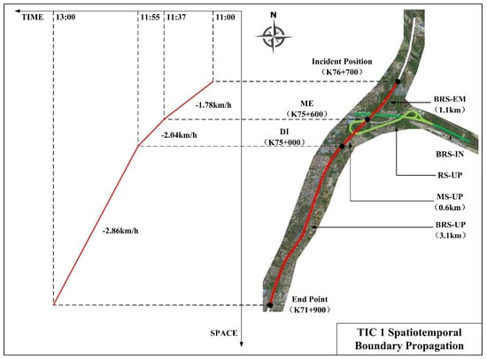
Figure 4.
TIC 1 spatiotemporal boundary propagation diagram.
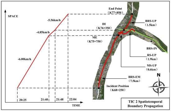
Figure 5.
TIC 2 spatiotemporal boundary propagation diagram.
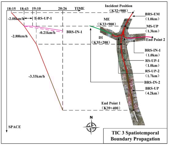
Figure 6.
TIC 3 spatiotemporal boundary propagation diagram.
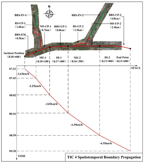
Figure 7.
TIC 4 spatiotemporal boundary propagation diagram.
Table 2.
Traffic condition of road sections in network covered by the congestions under traffic incident cases.
The spatiotemporal boundary propagation forecasting procedure works well for all four incident cases. However, to show its effectiveness, we compare the results obtained from the proposed method with these obtained from the field observations. Contributing to perfect RTMS (Real-time Traffic Management System), traffic flow data under abovementioned incident cases were recorded. In road sections inside the spatiotemporal boundary in each case, monitoring points (MPs) belonging to RTMS were deployed. Travel time of a spatiotemporal boundary reaching specific MPs and travel velocity after being impacted could be obtained through the diagrams given above, which is a predicted value in Table 3. Actual values of travel time and travel velocity could be obtained from the MPs directly. Abovementioned information is shown in Table 3.
Table 3.
Comparison between predicted values and actual values.
First of all, according to supervised traffic conditions, the proposed method makes all the judgements right, which is whether the congestion will spread to intersected road sections through the interchanges, by using boundary condition HNAC. In TIC 1, 2 and 4, merging traffic volume from intersected road to incident road is less than its HNAC value. Therefore, traffic flow in these intersected road sections is not affected by the incidents. In TIC 3, merging traffic volume is larger than the HNAC value of the incident road. In that, the intersected road section is congested; travel velocity dropped to 9.10 km/h. This proves the appropriateness and necessity of using HNAC in spatiotemporal boundary forecasting methods. The predicted values in MP1-K76+300, MP3-K73+400 and MP5-K33+400 equal to actual travel time, which shows a high accuracy of the method in incident road sections. According to data from BRSs of MP2-K73+500, MP4-K76+800, MP8-K17+100 and MP9-K13+100, the delays of actual travel time are 10.5%, 8.1%, 11.1%, 9.8%, respectively, which are close to each other. According to data from BRSs of MP6-K35+900 and MP7-E+150, the actual travel time delays are 16.2% and 14.8%, respectively.
Based on the above analysis, we could draw two conclusions. First, the accuracy (error of 10–15%) of this method in forecasting spatiotemporal boundary propagation time is adequate in practical work. Second, the prediction performances at different locations differs slightly. As reported in Section 3.2, higher heavy vehicle proportion leads to more instability in traffic flow, such as traffic conflicts brought by frequent overtaking. This phenomenon may further affect the prediction performances, and we will verify this hypothesis in Section 5. Moving to data of travel velocity, it could be found in MP5-K33+400, MP6-K35+900, MP8-K17+100 and MP9-K13+100 that predicted travel velocity values are accurate when road sections are blocked. However, in incident cases of MP1-K76+300, MP2-K73+500, MP3-K73+400, MP4-K76+800 and MP7-E+150, predicted travel velocity values are associated with large prediction errors. In this case, the proposed method is not quite appropriate for forecasting traffic velocity in spatiotemporal boundary propagation.
To further highlight the superiority of this spatiotemporal boundary propagation forecasting method, more analysis is done in this section. CTM-derived models introduced in Section 2 are mainly used to analyze traffic dynamic, oscillations and congestions in normal traffic flow, but in some circumstances, they could be used to analyze spatiotemporal boundary propagation [7,8,9,20,21,22]. In that, three CTM-derived models are chosen to specify the accuracy and efficiency of the method in this research, including Sakakibara’s CTM model [7], Meng’s model [21] and the original Daganzo model [6]. Using travel time of spatiotemporal boundary as a comparison objective, travel time derived from each model mentioned above is given below.
From Table 4, the advantages of proposed method are reflected in two points, compared to CTM-based models. First, the average accuracy of the proposed method (6.62%) is relatively higher (Sakakibara’s model: 20.4%, Meng’s model: 10.9%, Daganzo’s model: 22.2%). This might be attributed to the adoption of the general logistic-based volume–density model in Section 3.2, which could better describe the instable traffic flow brought by high heavy vehicle proportion, or other reasons. Second, some models failed in predicting traffic congestion in intersected road sections, which are Sakakibara’s and Meng’s. This is because these two models did not consider the clear boundary conditions like HNAC. We could not judge whether spatiotemporal boundary will uptrack to intersected road sections by just using the parameters shown in the proposed method, which could be directly observed using roadside monitoring facilities. Besides, compared to these CTM-based models, the method developed in this research shows more clarity and conciseness because the calculation procedures are all explicit, which makes the proposed method easier to be implemented in practice. Therefore, compared to CTM-derived models, the proposed method in this paper can better characterize the spatiotemporal boundary propagation in a real-world network.
Table 4.
Comparison between CTM-derived models and proposed method in this research.
5. Discussion
As depicted in Section 4, all values of the error in forecasting spatiotemporal boundary propagation time concentrate around two levels, 10% reported in MPs of MP2-K73+500, MP4-K76+800, MP8-K17+100 and MP9-K13+100, and, 15% reported in MPs of MP6-K35+900 and MP7-E+150. To be more specific, it could be found that 10% errors belong to TIC 1, TIC 2 and TIC 4; 15% errors belong to TIC 3. Moreover, errors reported in different MPs in the same TIC remain in the same level. Therefore, differences in forecasted spatiotemporal boundary propagation time may relate to the location of TIC. TIC 1 and TIC 2 happened in the adjacent two expressway sections, divided by three interchanges. The whole length of these two sections is no more than 6 km, which means the spacing between each interchange is very low. This phenomenon brings massive interweaving in these two sections. Besides, these two sections are connected with the expressways from Xi’an to Weinan, which are main arterials of coal transportation. Therefore, the heavy vehicle mixing ratio in these two sections is high, sometimes more than 30%. The length of expressway section where EC 4 happened is less than 3 km, and this section is the way leading to the airport, which also brings massive interweaving. In that, it could be speculated that traffic in sections where TIC 1, TIC 2 and TIC 4 happened is very much unstable. Compared to these three cases, the heavy vehicle mixing ratio in the expressway section where TIC 3 happened is much lower, no more than 10%. The length of this section is more than 6 km, and what remains is the traffic interweaving in a relatively low level. That means the stability of section where TIC 3 happened is higher than that of TIC 1, TIC 2 and TIC 4. Previous discussion proved the hypothesis in Section 4; the prediction performance difference derives from the traffic flow instability, not only caused by the large heavy vehicle mixing ratio. Therefore, when we put the proposed method into practice in expressway sections with high stability, 10% may be used as an error correction factor. When in expressway sections with low stability, 15% may be used as an error correction factor.
To further understand the practicality of this proposed method, we can look into the parameters and procedures it adopted and compare them to Sakakibara’s, Meng’s and the original Daganzo model analyzed in Section 4. In calculating the emergency-event-based congestion propagation velocity integrating general logistic-based volume–density model (Section 3.2) and HNAC (Section 3.3), parameters of free-flow velocity, block density, transitional density, traffic volume and heavy vehicle mixing ratio in certain road sections are used. Among these parameters, the previous three and the last one could be obtained according to historical traffic data. In a certain road section, they are constants. Traffic volume could be directly obtained through roadside monitoring facilities. However, Daganzo’s and Sakakibara’s models divide a road section, also merging and diverging area, into small homogeneous cells (e.g., 100 m), leading to oversized cell volume in a largescale road network [6,7]. Besides, it needs to analyze the traffic flow balance condition in each cell, at different time steps, which is complex and not easy to understand. In Meng’s model, the considered parameters volume reaches 29. Many of the parameters could not be observed directly, such as microscopic ones (e.g., longitudinal and lateral position of a certain vehicle) [21]. Therefore, compared to these CTM-based models, this HNAC based proposed method shows its superiority in explicitness and practicality.
To make this proposed method better in application, reasons that may cause the error in prediction accuracy should be discussed in order to provide a basis in future model improvement. From Table 3, it could be noticed that time consumption of spatiotemporal boundary reaching upstream or intersected BRSs obtained from the forecast method are less than the actual value. This could be understood in some phenomenon observed in real road emergency. In CTM-derived models [5,6], origin-destination (O-D) data of drivers are assumed to be unchanged. In ordinary conditions, this assumption meets real traffic situations. In emergency events, some drivers will change their travel routes to evade congestion, which will relieve the spatiotemporal boundary propagation to some extent. Although the proportion of these drivers is relatively small according to field observation, it does affect the spatiotemporal boundary propagation. As criticized by microscopic traffic studies [50], macroscopic methods do not always take detailed driving behaviors into consideration. In this research, a unique phenomenon should be noticed. In the expressway network of this research, drivers tend to change their lanes in higher frequency to obtain relatively front positions when traffic becomes congested. This phenomenon also has some impact on spatiotemporal boundary propagation.
6. Conclusions
In related literatures, how to make an accurate judgement on whether the congestion (spatiotemporal boundary) will spread into intersected expressway sections through an interchange is not answered. Therefore, explicit and practical methods on forecasting spatiotemporal boundary propagation of emergency-event-based congestion in expressway network have not been found in related works. To make up this shortage, a critical element, HNAC—referring to the upper limit of traffic volume merging into a target road from an intersected road through the on-ramp in an interchange—is used to answer the key problem. Combing the spatiotemporal boundary propagation direction-based expressway network subdivision method, kinetic wave theory, and logistic-based volume–density model, a new method forecasting emergency-event-based traffic congestion propagation in an expressway network is built. To prove the practicality and efficiency of the method, it is implemented in four traffic incident cases and corresponding real road data. By comparing predicted results with real road recorded information, the accuracy (10% in expressway sections with high traffic stability, 15% in expressway sections with low traffic stability) of this method in forecasting spatiotemporal boundary propagation time is adequate in practical work. Furthermore, the method proposed in this research is proven to be clearer and more concise than CTM-derived models in analyzing spatiotemporal boundary propagation, owing to the adoption of HNAC, which is more practical.
However, works in two aspects are still needed. The first one is the providing of a clear definition of traffic stability, which could offer basis in forecast method error correction. Besides, forecast error is related to drivers’ small-scale bypassing and lane-changing behaviors under emergency events. Therefore, further studies should focus on involving microscopic driving behaviors into forecasting spatiotemporal boundary propagation in expressway networks.
Author Contributions
Conceptualization, X.L. and T.L.; data curation, X.L.; funding acquisition, X.L.; investigation, J.W. and T.L.; methodology, X.L. and J.W.; writing—original draft, X.L.; writing—review & editing, J.W., T.L. and J.X. All authors have read and agreed to the published version of the manuscript.
Funding
This study is supported by Scientific and Technological Research Program of Chongqing Municipal Education Commission (Grant No. KJQN202100718), Scientific and Technological Research Program of Chongqing Jiaotong University (Grant No. 20JDKJC-B001), and Ningxia Transport Science & Technology Project (Grant No. 202100182).
Institutional Review Board Statement
Not applicable.
Informed Consent Statement
Not applicable.
Data Availability Statement
The data in this study is available under the permission of all the authors.
Conflicts of Interest
The authors declare no conflict of interest.
References
- Morales, J.M. Analytical procedures for estimating freeway traffic congestion. Public Road 1986, 50, 55–61. [Google Scholar]
- Newell, G.F. A simplified theory of kinematic waves in highway traffic, part I: General theory. Transp. Res. Part B Methodol. 1993, 27, 281–287. [Google Scholar] [CrossRef]
- Newell, G.F. A simplified theory of kinematic waves in highway traffic, part II: Queueing at freeway bottlenecks. Transp. Res. Part B Methodol. 1993, 27, 289–303. [Google Scholar] [CrossRef]
- Newell, G.F. A simplified theory of kinematic waves in highway traffic, part III: Multi-destination flows. Transp. Res. Part B Methodol. 1993, 27, 305–313. [Google Scholar] [CrossRef]
- Daganzo, C.F. The cell transmission model: A dynamic representation of highway traffic consistent with the hydrodynamic theory. Transp. Res. Part B Methodol. 1994, 28, 269–287. [Google Scholar] [CrossRef]
- Daganzo, C.F. The cell transmission model, part II: Network traffic. Transp. Res. Part B Methodol. 1995, 29, 79–93. [Google Scholar] [CrossRef]
- Sakakibara, T.; Honda, Y.; Horiguchi, T. Effect of obstacles on formation of traffic jam in a two-dimensional traffic network. Phys. A Stat. Mech. Appl. 2000, 276, 316–337. [Google Scholar] [CrossRef]
- Tian, J.F.; Yuan, Z.Z.; Jia, B.; Fan, H.Q.; Wang, T. Cellular Automaton Model in the Fundamental Diagram Approach Reproducing the Synchronized Outflow of Wide Moving Jams. Phys. Lett. A 2012, 376, 2781–2787. [Google Scholar] [CrossRef]
- Wang, Z.J.; Ma, S.F.; Jiang, R.; Tian, J. A cellular automaton model reproducing realistic propagation speed of downstream front of the moving synchronized pattern. Transp. B Transp. Dyn. 2019, 7, 295–310. [Google Scholar] [CrossRef]
- Cao, J.; Hadiuzzaman, M.; Qiu, T.Z.; Hu, D. Real-time queue estimation model development for uninterrupted freeway flow based on shockwave analysis. Can. J. Civ. Eng. 2015, 42, 153–163. [Google Scholar] [CrossRef]
- Cheng, Y.; Qin, X.; Jin, J.; Ran, B. An Exploratory Shockwave Approach to Estimating Queue Length Using Probe Trajectories. J. Intell. Transp. Syst. 2012, 16, 12–23. [Google Scholar] [CrossRef]
- Lawson, T.W.; Lovell, D.J.; Daganzo, C.F. Using Input-Output Diagram to Determine Spatial and Temporal Extents of a Queue Upstream of a Bottleneck. Transp. Res. Rec. J. Transp. Res. Board 1997, 1572, 140–147. [Google Scholar] [CrossRef] [Green Version]
- Mehran, B.; Nakamura, H. Implementing travel time reliability for evaluation of congestion relief schemes on expressways. Transp. Res. Rec. J. Transp. Res. Board 2009, 2124, 137–147. [Google Scholar] [CrossRef]
- Stephanopoulos, G.; Michalopoulos, P.G. Modeling and analysis of traffic queue dynamics at signalized intersections. Transp. Res. Part A Gen. 1979, 13, 295–307. [Google Scholar] [CrossRef]
- Dudek, C.L.; Richards, S.H. Traffic Capacity Through Urban Freeway Work Zones in Texas. Transp. Res. Rec. J. Transp. Res. Board 1982, 869, 14–18. [Google Scholar]
- Jin, W.L.; Gan, Q.J.; Gayah, V.V. A kinematic wave approach to traffic statics and dynamics in a double-ring network. Transp. Res. Part B Methodol. 2013, 57, 114–131. [Google Scholar] [CrossRef]
- Nam, D.D.; Drew, D.R. Analyzing Freeway Traffic under Congestion: Traffic Dynamics Approach. J. Transp. Eng. 1998, 124, 208–212. [Google Scholar] [CrossRef]
- Wirasinghe, S.C. Determination of Traffic Delays from Shock-wave Analysis. Transp. Res. 1978, 12, 343–348. [Google Scholar] [CrossRef]
- Wu, X.K.; Liu, H.X. A shockwave profile model for traffic flow on congested urban arterials. Transp. Res. Part B Methodol. 2011, 45, 1768–1786. [Google Scholar] [CrossRef]
- Fei, L.; Zhu, H.B.; Han, X.L. Analysis of traffic congestion induced by the work zone. Phys. A Stat. Mech. Appl. 2016, 450, 497–505. [Google Scholar] [CrossRef]
- Meng, Q.; Weng, J.X. An Improved Cellular Automata Model for Heterogeneous Work Zone Traffic. Transp. Res. Part C Emerg. Technol. 2011, 19, 1263–1275. [Google Scholar] [CrossRef]
- Tian, J.F.; Jia, N.; Zhu, N.; Jia, B.; Yuan, Z.Z. Brake Light Cellular Automaton Model with Advanced Randomization for Traffic Breakdown. Transp. Res. Part C Emerg. Technol. 2014, 44, 282–298. [Google Scholar] [CrossRef]
- Liu, X.L.; Xu, J.L.; Dong, Y.P.; Ru, H.; Duan, Z. Defining Highway Node Acceptance Capacity (HNAC): Theoretical Analysis and Data Simulation. J. Adv. Transp. 2020, 2020, 8939621. [Google Scholar] [CrossRef] [Green Version]
- Ban, X.; Pang, J.S.; Liu, H.X.; Ma, R. Continuous-time point-queue models in dynamic network loading. Transp. Res. Part B Methodol. 2012, 46, 360–380. [Google Scholar] [CrossRef]
- Liu, H.X.; Wu, X.K.; Ma, W.T.; Hu, H. Real-time queue length estimation for congested signalized intersections. Transp. Res. Part C Emerg. Technol. 2009, 17, 412–427. [Google Scholar] [CrossRef]
- Nie, X.; Zhang, H.M. Delay-function-based link models: Their properties and computational issues. Transp. Res. Part B Methodol. 2005, 39, 729–751. [Google Scholar] [CrossRef]
- Lighthill, M.J.; Whitham, G.B. On Kinematic Waves II-A Theory of Traffic Flow on Long Crowded Roads. Proc. R. Soc. A Math. Phys. Eng. Sci. 1955, 229, 317–345. [Google Scholar]
- Richards, P.I. Shock Waves on the Highway. Oper. Res. 1956, 4, 42–51. [Google Scholar] [CrossRef]
- Bagnerini, P.; Rascle, M. A multi-class homogenized hyperbolic model of traffic flow. SIAM J. Math. Anal. 2003, 35, 949–973. [Google Scholar] [CrossRef]
- Colombo, R.M. A 2 × 2 hyperbolic traffic flow model. Math. Comput. Model. 2002, 35, 683–688. [Google Scholar] [CrossRef]
- Hoogendoorn, S.P.; Bovy, P.H.L. Multiclass macroscopic traffic flow modelling: A multilane generalisation using gas-kinetic theory. In Proceedings of the 14th International Symposium on Transportation and Traffic Theory, Jerusalem, Israel, 20–23 July 1999. [Google Scholar]
- Holland, E.N.; Woods, A.W. A continuum model for the dispersion of traffic on two-lane roads. Transp. Res. Part B Methodol. 1997, 31, 473–485. [Google Scholar] [CrossRef]
- Laval, J.A.; Daganzo, C.F. Multi-lane hybrid traffic flow model: A theory on the impacts of lane-changing maneuvers. In Proceedings of the 84th Transportation Research Board’s Annual Meeting, Washington, DC, USA, 9–13 January 2005. [Google Scholar]
- Munjal, P.K.; Hsu, Y.S.; Lawrence, R.L. Analysis and validation of lane-drop effects on multi-lane freeways. Transp. Res. 1971, 5, 257–266. [Google Scholar] [CrossRef]
- Munjal, P.K.; Pipes, L.A. Propagation of on-ramp density perturbations on unidirectional two- and three-lane freeways. Transp. Res. 1971, 5, 241–255. [Google Scholar] [CrossRef]
- Tampère, C.M.J.; Van Arem, B.; Hoogendoorn, S.P. Gas kinetic traffic flow modelling including continuous driver behavior models. Transp. Res. Rec. J. Transp. Res. Board 2003, 1852, 231–238. [Google Scholar] [CrossRef]
- Comert, G.; Cetin, M. Queue length estimation from probe vehicle location and the impacts of sample size. Eur. J. Oper. Res. 2009, 197, 196–202. [Google Scholar] [CrossRef]
- Hao, P.; Ban, X.G. Long queue estimation for signalized intersections using mobile data. Transp. Res. Part B Methodol. 2015, 82, 54–73. [Google Scholar] [CrossRef] [Green Version]
- Hao, P.; Ban, X.G.; Guo, D.; Ji, Q. Cycle-by-cycle intersection queue length distribution estimation using sample travel times. Transp. Res. Part B Methodol. 2014, 68, 185–204. [Google Scholar] [CrossRef]
- Lee, Y.; Wei, C.H.; Chao, K.C. Evaluating the Effects of Highway Traffic Accidents in the Development of a Vehicle Accident Queue Length Estimation Model. Int. J. Intell. Transp. Syst. Res. 2016, 16, 26–38. [Google Scholar] [CrossRef]
- Liu, X.L.; Xu, J.L.; Li, M.H.; Wei, L.; Ru, H. General-Logistic-Based Speed-Density Relationship Model Incorporating the Effect of Heavy Vehicles. Math. Probl. Eng. 2019, 1934, 6039846. [Google Scholar] [CrossRef] [Green Version]
- TRB. Highway Capacity Manual 2010; Transportation Research Board: Washington, DC, USA, 2010. [Google Scholar]
- Edie, L.C. Car-following and steady-state theory for noncongested traffic. Oper. Res. 1961, 9, 66–76. [Google Scholar] [CrossRef]
- Greenberg, H. An analysis of traffic flow. Oper. Res. 1959, 7, 79–85. [Google Scholar] [CrossRef]
- Greenshields, B.D.; Bibbins, J.R.; Channing, W.S.; Miller, H.H. A study of traffic capacity. Transp. Res. Rec. J. Transp. Res. Board 1935, 14, 448–477. [Google Scholar]
- May, A.D. Traffic Flow Fundamentals; Prentice Hall: Englewood Cliffs, NJ, USA, 1990. [Google Scholar]
- Sun, L.; Zhou, J. Development of multiregime speed-density relationships by cluster analysis. Transp. Res. Rec. J. Transp. Res. Board 2005, 1934, 64–71. [Google Scholar] [CrossRef]
- Underwood, R.T. Speed, volume, and density relationship: Quality and Theory of Traffic Flow. Transp. Res. Board 1961, 141–188. Available online: https://trid.trb.org/view/115231 (accessed on 2 November 2021).
- Wang, H.Z.; Li, J.; Chen, Q.Y.; Ni, D. Logistic modeling of the equilibrium speed-density relationship. Transp. Res. Part A Policy Pract. 2011, 45, 554–566. [Google Scholar] [CrossRef]
- Papageorgiou, M. Some remarks on macroscopic traffic flow modeling. Transp. Res. Part A Policy Pract. 1998, 32, 323–329. [Google Scholar] [CrossRef]
Publisher’s Note: MDPI stays neutral with regard to jurisdictional claims in published maps and institutional affiliations. |
© 2021 by the authors. Licensee MDPI, Basel, Switzerland. This article is an open access article distributed under the terms and conditions of the Creative Commons Attribution (CC BY) license (https://creativecommons.org/licenses/by/4.0/).