Abstract
The concept of vehicle automation is a promising approach to achieve sustainable transport systems, especially in an urban context. Automation requires the integration of learning-based approaches and methods in control theory. Through the integration, a high amount of information in automation can be incorporated. Thus, a sustainable operation, i.e., energy-efficient and safe motion with automated vehicles, can be achieved. Despite the advantages of integration with learning-based approaches, enhanced vehicle automation poses crucial safety challenges. In this paper, a novel closed-loop matching method for control-oriented purposes in the context of vehicle control systems is presented. The goal of the method is to match the nonlinear vehicle dynamics to the dynamics of a linear system in a predefined structure; thus, a control-oriented model is obtained. The matching is achieved by an additional control input from a neural network, which is designed based on the input–output signals of the nonlinear vehicle system. In this paper, the process of closed-loop matching, i.e., the dataset generation, the training, and the evaluation of the neural network, is proposed. The evaluation process of the neural network through data-driven reachability analysis and statistical performance analysis methods is carried out. The proposed method is applied to achieve the path following functionality, in which the nonlinearities of the lateral vehicle dynamics are handled. The effectiveness of the closed-loop matching and the designed control functionality through high fidelity CarMaker simulations is illustrated.
1. Introduction and Motivation
In recent years, advanced driver-assistance systems have become widespread among modern vehicles. These systems are focused on assisting the driver of the vehicle (e.g., lane-keeping assist system, cruise control). The main role of these systems is to make everyday traffic safer and to reduce the accidents caused by human errors. However, many problems cannot be solved using only the mentioned systems. One of the main issues to be addressed is the loss of time due to driving. An average American worker spends more than an hour a day driving a vehicle [1]. The main problem is that this time cannot be usefully spent by the driver. In the future, highly automated/autonomous vehicles will take over the burden of driving, which will allow the passengers to spend the traveling time with other productive activities. Moreover, autonomous vehicles will have a major impact on society. Self-driving vehicles will increase the living standards of many people, and personal freedom can be also increased [2]. Furthermore, maintaining the same level of mobility will not require owning a car, which will result in a significant reduction in spending.
In addition, traffic jams have a number of negative effects, such as increased travel time, increasing fuel consumption [3], and emission [4]. These effects can be significantly reduced with autonomous vehicles [5]. Moreover, other advantages of autonomous vehicles are the reduction in the safe traveling distance and the higher speed limits, which decrease traffic jams and traveling times. Previously, some problems were presented that are strongly related to energy usage and emission. Autonomous vehicles play a key role in reducing these effects. Due to the mentioned advantages, many automotive companies and researchers are dealing with issues related to autonomous vehicles. The main criterion for the widespread of the fully autonomous vehicle is the safe and reliable operation in any traffic situation. The development of autonomous vehicle technologies has grown significantly in the last decade. The system, which is responsible for the operation of autonomous vehicles, can be divided into several layers [6]. For example, the sensing layer accurately evaluates the given traffic situation; another layer, the decision-making one, is responsible for the motion planning of the car. Finally, the control algorithm guarantees the accurate trajectory tracking of the vehicle.
In the future era of autonomous vehicles, optimal traffic control algorithms will play a key role (e.g., smart intersections). These algorithms provide reference trajectories for the vehicles. By tracking these trajectories, an energy optimal traffic flow can be achieved. Therefore, in order to reach this energy optimal traffic flow, the control systems on the vehicle must guarantee accurate tracking performance.
Furthermore, it can be said that a number of problems arise during the control design. One of the main problems is that the system parameters are not known exactly known. This means that the control algorithm may not be satisfying the energy minimum requirement. In this paper, a novel method is presented for the control design, which can improve the performance of the nominal control system.
One of the most difficult challenges is the modeling process of a system since it may contain several nonlinearities and uncertain parameters. Moreover, in several cases, nonlinearities are difficult to handle [7]. In recent years, several approaches have been developed to solve this problem. The first group includes methods, which linearize the system. The simplest approach is when only one linear system is determined. In other cases, several linear systems are determined in numerous operating points of the nonlinear system. Furthermore controllers can be designed for the defined linear systems. Using the resulted set of controllers, and based on the actual information of the system, the controller parameters can be calculated as an interpolation. This method is called, in the literature, gain-scheduling control [8]. Although the control design of this method is simple, the performance of this method may be poor. There can be found polytopic system–based algorithms, such as the linear parameter-varying framework (LPV) [9]. The second group consists of algorithms, in which the nonlinearities of the system are taken into account during the modeling phase. The stability analysis of a polynomial system is presented in [10]. In [11], a control problem is introduced, using a (sum-of-squares) SOS programming method. In these methods, the model contains nonlinearities, which makes the control design a challenging task. The nonlinearities of the system can be taken into account in several ways, e.g., the nonlinear model predictive control method (NMPC) [12]. An advantage of the MPC approach is that it can take into account the bounds of the states of the system, by which the stability of the controlled plant is guaranteed. These bounds can be determined by computing the reachability sets of the system; see [13].
The third group is the classical methods. A possible approach to deal with the nonlinearities of the system is the feedback linearization; see [14,15]. The feedback linearization process requires an accurate description of the system. However, in many cases, it is not available or cannot be determined since the system may contain high nonlinearities and uncertainties. Moreover, if it is available, the inversion of the system is also a difficult task to achieve; see [16].
With the increase in the computation capacity of computers, new fields have come into view, such as data-driven and machine learning–based approaches. Several methods have been developed, using a combination of the classical and machine learning–based approaches. In [9], a method is presented in which an (LPV) approach is combined with the results of machine learning–based technique. The reachability sets are computed for the controlled vehicle, using data-driven analyses and a machine learning algorithm, and the results are used in a model predictive approach, which guarantees the trajectory tracking [17]. Furthermore, neural networks can be also used during feedback linearization. In [18], a feedback linearization method is presented for the tracking performance based on neural networks. Moreover, neural network-based feedback linearization is used in many fields of vehicle control (such as suspension control [19], and longitudinal control [20]). Feedback linearization is made for a nonlinear system with unknown dynamics, using the reinforcement learning technique [21]. Moreover, in [22], an input–output linearization method is presented for robotic applications by reinforcement learning. One of the main advantages of the proposed methods is the fact that an accurate system description is not necessary during the linearization process.
The main advantage of the first three methods is that the stability of the system can be guaranteed in the operation range of the system. However, the accurate control design requires the exact knowledge of the given system, which is a challenging task in several cases. Although the machine learning algorithms can boost the performance of the controlled plant, there is no analytical proof to guarantee their stability, which is a major issue in safety-critical systems. Some papers deal with this problem, e.g., in the work of [23], a method is proposed for computing the reliability of the neural networks.
In this paper, a novel model matching-based control approach is presented, using a machine learning–based algorithm. The control algorithm is beneficial for those systems, which are of high complexity and exposed to parameter uncertainty. A contribution of the paper is that the level of control performance through learning-based approaches is improved, and similarly, stable motion of the vehicle through the operation of the control is guaranteed. Thus, one of the main disadvantages of several neural network–based control methods can be avoided, i.e., lack of stability. A further contribution of the paper, in contrast to the former methods in the literature, is that the improvement of the performance level through the extension of the simplified design methods based on the nominal linear system model is carried out. The nominal model of the system is considered to be known since the dynamics of the original system is adjusted to the nominal model. In this way, the complexity of the control design process is reduced and the performance of the closed-loop system can be guaranteed without taking into account the uncertainties and the unmodeled dynamics of the system. The presented control strategy is implemented in Matlab/CarMaker environments, and its efficiency is demonstrated through a comprehensive simulation example.
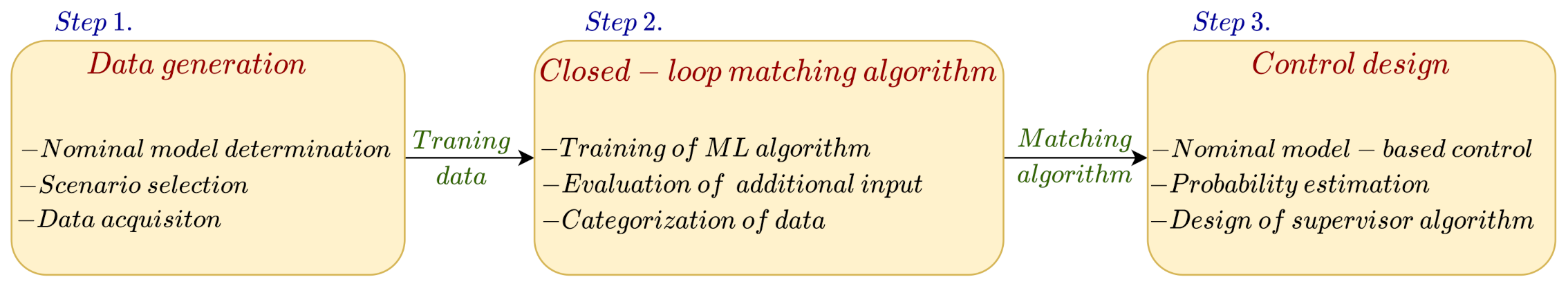
The structure of the proposed algorithm is shown in Figure 1, which can be divided into three main parts. The first block contains the steps of the data generation. Firstly, a nominal model is selected, which is the basis of the matching problem. Then, the test scenarios and the simulations are considered. The appropriately selected scenarios are essential in order to ensure that the collected dataset covers the full operating range of the system. Using the nominal model and the scenarios, data acquisition is performed. In the second part of the algorithm, the reachability sets are computed based on the collected data, and also the machine learning–based method is presented for the additional steering angle computation. Then, the reliability estimation for the network is determined. Finally, the main goal of the third part is the control design. The lateral controller is designed, using solely the nominal model. Moreover, the last part is the calculation of the reference signal, which takes into account the computed stability sets in order to ensure the stability of the nonlinear system.
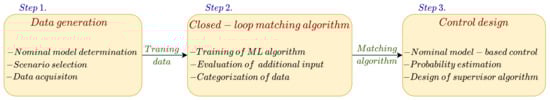
Figure 1.
Methodological scheme of the control method.
The paper is structured as follows: In Section 2, the construction of the nominal model is presented, which is used both in the training process of the neural network and during the reference signal generation. Moreover, this section describes the acquisition of the dataset, which is used to train and evaluate the closed-loop matching neural network. Section 3 presents the computation of the stability sets. Moreover, the reliability estimation of the neural network is also presented in this section. The model-based reference signal generation is presented in Appendix A. In Section 4, a comprehensive simulation example is given to show the efficiency and the operation of the proposed control algorithm. Finally, the paper is concluded in Section 5.
2. Closed-Loop Matching Using a Neural Network-Based Approach
In this paper, the effectiveness of the proposed method is demonstrated through a vehicle-oriented problem, in which the model matching process is carried out in terms of the yaw rate of the vehicle. In Figure 2, the scheme of the closed-loop matching is presented. The goal is to compute an additional input signal by which the output signals () become identical. In this case, means an additional steering angle, and () are the yaw rates of the nominal and nonlinear system.
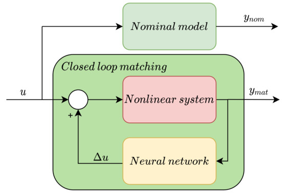
Figure 2.
Structure of the closed-loop matching.
In the following subsection, the construction of the nominal model is presented, which serves as a base of the neural network-based closed-loop matching and the model-based reference generation. The nominal model consists of two main parts: the lateral vehicle, which is based on the two-wheeled bicycle model, and the steering system, which is modeled by a first-order term.
2.1. Lateral Vehicle Model
The main idea behind this model is to replace the front and rear wheels of the vehicle by one wheel, which is placed on the axis of symmetry of the vehicle. Basically, it consists of two equations: the first describes the lateral motion of the car, while the second equation describes its yaw motion (see [24]):
where m is the mass of the car, are geometrical parameters and denotes the yaw inertia. Moreover, is the side-slip angle. The longitudinal velocity of the vehicle is (), the road wheel angle is denoted by and is the yaw rate. The lateral tire forces can be computed as follows:
where is the cornering stiffness of the tires, and represents the side-slip angles of the tires. Using (1)–(3), a transfer function () can be determined. The input of the system is the steering angle , and the output is the yaw rate () of the vehicle. Using the Laplace transform of the output and the Laplace transform of the input , the following transfer function can be formed:
Note that during the construction of the nominal model, several parameters of the vehicle are unknown, such as the cornering stiffness and the yaw inertia. The longitudinal velocity can change during the simulations, but this value is fixed during the construction of the nominal model. The second part of the nominal model is the steering system. In autonomous vehicles, the steering system has a significant effect on the lateral dynamics, due to the delays caused by the electric motor and its inertia. This dynamics can be modeled by a simple first-order term [25], as follows:
where is the time delay and provides the steady-state gain of the steering system.
2.2. Computation of the Inverse Model
The nominal linear model consists of the presented two parts: lateral vehicle and the steering system. This model can be transformed into a transfer function, whose input is the steering angle () and its output is the yaw rate () of the vehicle. In the first step, the inverse of the nominal model is calculated [26]:
The computation of the inverse model can be challenging [27]. Furthermore, after the inversion, the system may not be causal. In order to meet this issue, a prefilter is used.
where gives the prefilter, which is used in order to deal with non-causalities. The discretization process is made, using Tustin’s method [28].
where denotes the ith pole of the continuous system, while represents the discrete poles of the discretized system. Furthermore, T is the discretization time. Finally, the calculated discretized inverse model is used during the neural network-based matching process, which is presented in the next subsection.
2.3. Data Generation for the Neural Network
In this subsection, the data generation is presented for the neural network, which is responsible for closed-loop matching. The goal of the matching process is to compute an additional steering angle () by which the closed-loop system matches the behavior (output) of the nominal model, which is presented in Section 2.1. Since the system is influenced by high nonlinearities and the parameters are not accurately known, the computation of is not a straightforward task. In order to compute the additional steering angle, an iterative process is presented, which cannot be applied in real-time application. The main role of the neural network is to calculate the additional steering angle for the nonlinear system based on the measurable states of the system in real-time application. In the following, more details are given for the data generation process.
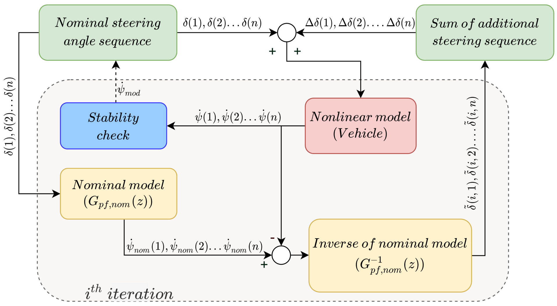
In Figure 3, the data generation process is presented. The basis of the data generation is the deviation between the output (yaw rate) of the nominal model and the measured yaw rate of the nonlinear model by which a nominal steering angle sequence () is determined, using the inverse of the nominal model. This error function is computed at each iteration step. After an iteration step, the resulting additional steering angle () sequence is added to the previously determined sequence. The training dataset consists of the measurable data, which are collected directly from the nonlinear system at the last iteration step. In the following, more details are given on the iterative algorithm.
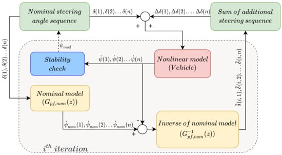
Figure 3.
Structure of the data generation.
In the first iteration step, the value of the additional steering angle is set to zero and the yaw rate is computed from the nominal model. Then, the error between the yaw rate signal can be computed, . Using the error value and the inverse of the nominal model, the additional steering angle is computed and saved. In the second iteration step, the input of the vehicle is modified as follows: . Note that the yaw rate of the vehicle and the calculated yaw rate using the nominal model may not match. This phenomenon can be explained by the fact that is computed using only the nominal model. The iterative process with which the additional steering angle is computed, is formed as follows:
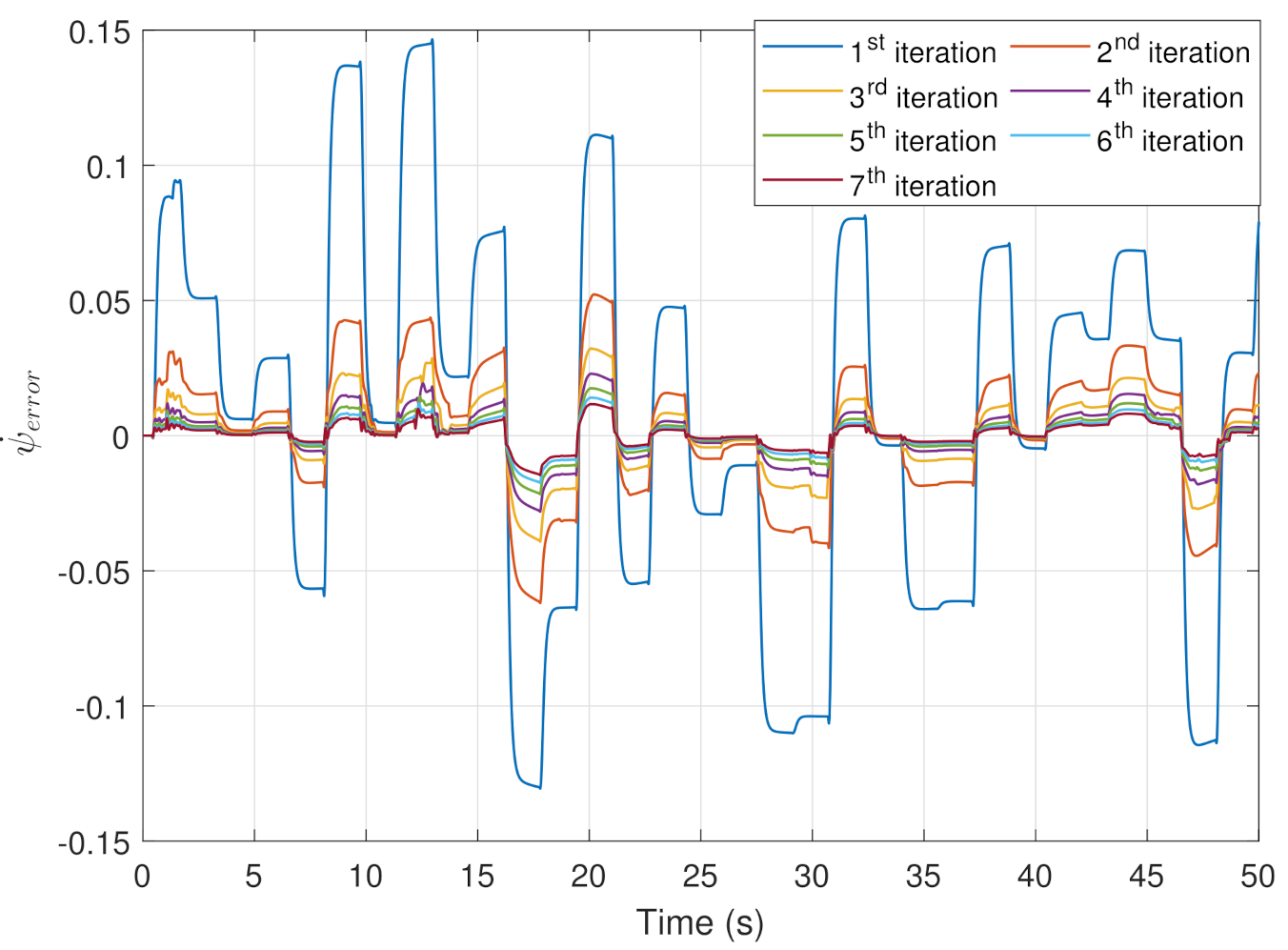
where n gives the number of iterations. The iterations must be made until the maximum of the yaw rate error reaches an appropriately small value . In Figure 4, an example is presented for the results of the iteration process. In Figure 4, it is shown that in the first iteration step, the error between the nominal and the nonlinear model is the highest, which is represented with the blue line. This error value decreases with the increase in the iterations.
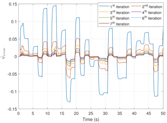
Figure 4.
Results of the iteration processes.
Since the nominal model does not contain information on the stability regions of the nonlinear model, a checking process is applied in the data generation, which can modify the nominal steering angle sequence. This means that if the vehicle loses its stability, the steering angle is modified in which the longitudinal velocity and the maximum value of the yaw rate () are taken into account. During data generation for the training set, the maximum value of the nominal control input sequence to preserve the stable motion of the vehicle is bounded. The bound through a maximum steering angle is defined, whose angle based on the lateral vehicle model is computed. If the vehicle model during the data generation on a section of a scenario is not able to perform the reference yaw rate value, the maximum steering angle by a predefined value, e.g., 10%, is decreased. The main role of this part is to ensure the stable motion of the vehicle. The following pseudo algorithm presents the data generation for the nth step.
The presented iterative process is used in the simulations, which provide the dataset for the training process of the neural network. The whole iteration process is performed until the error between the nominal and the measured yaw rate reaches a predefined small value . In the example of this paper, the value of is set to 0.01. During the simulations, the longitudinal velocity of the vehicle varies between and the vehicle is driven along different tracks. Using Algorithm 1, the additional steering angle sequence is determined and saved. Note that the additional control input has an influence on the states of the vehicle. This means that the training dataset should contain the effect of the additional steering angle because the neural network calculates the additional steering angle, using the measured states. In order to solve this problem, the input of the neural network is the states of the vehicle, which is saved at the last iteration step. The following variables are measured and collected from the simulations:
- Longitudinal velocity ().
- Acceleration ().
- Angular velocities ().
- Steering angle ().
- Nominal steering angle from the inverse model ().
- Additional steering angle ().
In this way, more than 1 million distinct instances are gathered. Note that only that the signals are used, which are available from the onboard sensors. In summary, the value of the additional steering angle cannot be determined in only one step, due to uncertain parameters and high nonlinearities.
| Algorithm 1: Computation of the steering angle. |
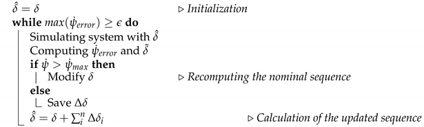 |
2.4. Training of the Neural Network
It is mentioned that the closed-loop matching is achieved through the computation of an additional steering angle, which is generated using an iterative algorithm. Nevertheless, the iterative algorithm cannot be used in real-time applications. In order to meet this issue, a neural network is used to calculate the additional steering angle, using the measurable states of the vehicle. The training dataset of the network is created, using the iterative algorithm, which is detailed in Section 2.3. The inputs of the network are the measurable states, and the output is the computed additional steering angle. In this subsection, the training process is presented.
The neural networks can be divided into three main layers: the input layer, the hidden layers, and finally the output layer. Each layer consists of neurons, more precisely, weights and activation functions. Before the training process, the number of neurons and hidden layers must be determined. In this paper, the parameters of the implemented neural network are determined, using the so-called k-fold cross-validation technique [29]. The following table shows the parameters of the trained neural network.
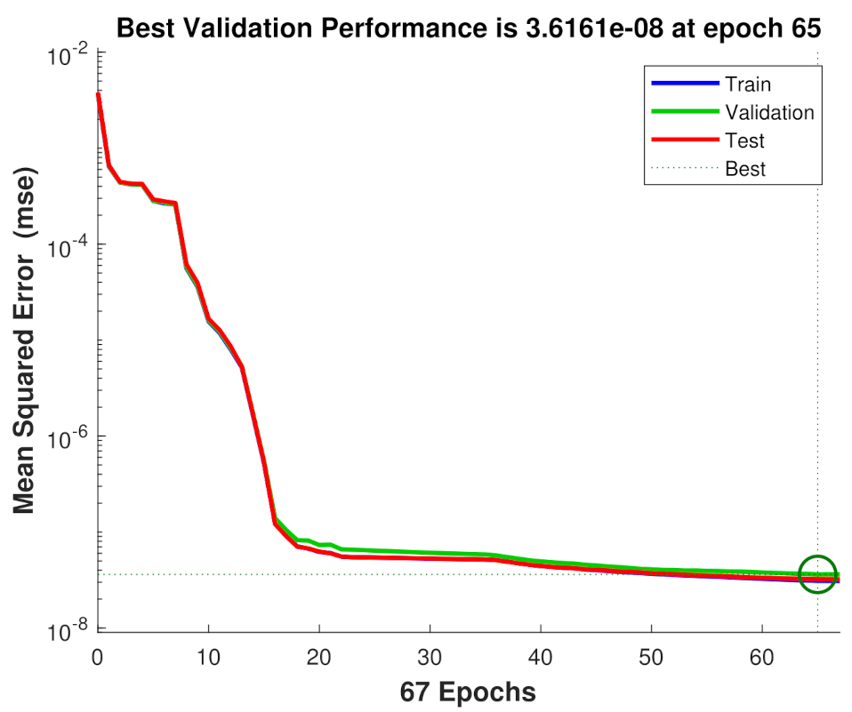
In Table 1, the main parameters of the neural network are presented, and during the training process, a Levenberg–Marquardt algorithm is used. The training process of the neural network-based additional control input computation algorithm is performed using Matlab Neural Network Toolbox [30]. Figure 5 illustrates the loss function of the training process.

Table 1.
Parameters of the trained neural network.

Figure 5.
Loss function of the training process.
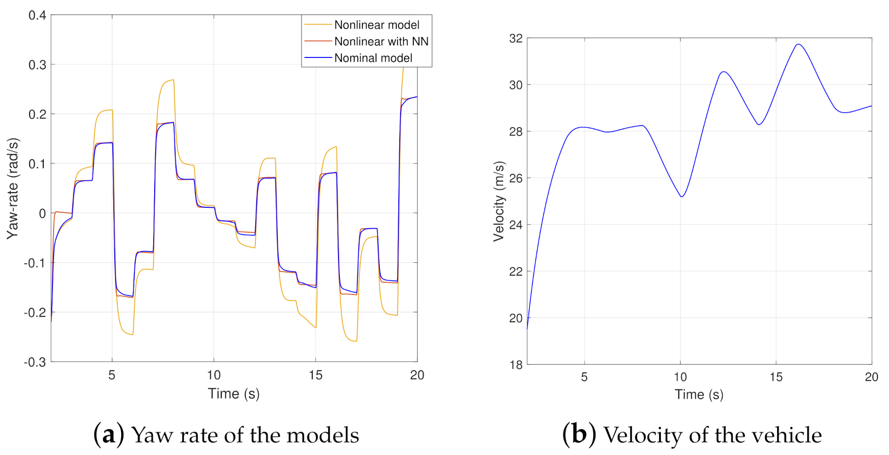
Figure 6 show a test scenario, in which the reference steering angle is set to randomly chosen values and also the velocity of the vehicle varies during the scenario. The goal is to reach the yaw rate of the nominal model by adding the additional steering angle to the nominal control input. The additional steering angle, computed by the presented neural network is evaluated at each time step during the operation of the implemented algorithm.
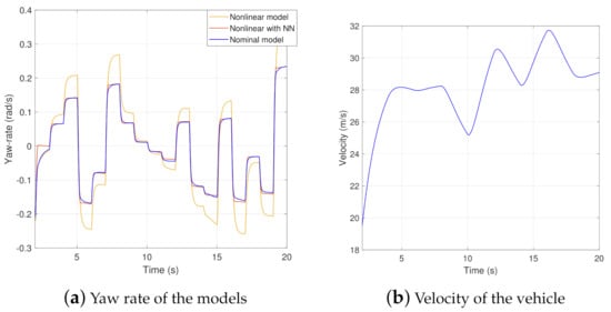
Figure 6.
Validation of the neural network.
In Figure 6, the output of the nominal model can be seen (blue line) and also the output of the nonlinear model with the additional steering angle is presented (red line). It can be seen that the outputs of the systems are nearly the same. The maximal error between the two yaw rate signals is only about ≈0.01 rad/s, which is a reasonably small value. Moreover, the yellow line represents the output of the nonlinear system without the additional steering angle, which significantly differs from the output of the nominal model. Therefore, the neural network–based closed-loop matching algorithm is able to fit the output of the nonlinear system to the nominal system.
3. Evaluation of the Neural Network–Based Closed-Loop Matching
It was shown that the neural network-based matching method is able to modify the dynamics of the nonlinear system by computing an additional steering angle. However, the neural networks may provide outputs, which destabilize the closed-loop system. It has two main reasons as follows:
- The training dataset contains data points that belong to the unstable regions of the vehicle.
- The training dataset may not completely cover the operating range of the system, or the fitting error of the neural network is too high.
As a first step, the acquired dataset is divided into two subsets, according to the stability of the instances. This categorization is carried out by using a data-driven approach. In the second step, the performances of the neural network are evaluated. The result of the evaluation is also two subsets: the first one contains those cases, where the closed-loop with the neural network satisfies the criterion, and the second one consists of the rest of the dataset. Both categorization methods are presented in the following subsection.
3.1. Categorization of the Dataset
3.1.1. Determination of Stability Regions
However, the stability of the closed-loop system cannot be proved analytically, which means that there is no guarantee that the modified system remains stable in every possible case. In order to overcome this issue, the reachability set analysis of the closed-loop system is performed, which is detailed in this subsection. The reachability sets of a dynamical system can be defined as follows. It is given a continuous-time system with initial condition . It is considered the set of reachable states with inputs u whose components have unit-energy as follows [31]:
The computation of the reachability sets is a challenging problem, especially for highly nonlinear systems. The computation becomes more difficult in cases where a neural network–based algorithm is involved in the closed-loop system. Therefore, in this paper, a data-driven reachability set computation is used. Briefly, the algorithm divides the dataset into two main groups (acceptable and unacceptable instances). If the given instance satisfies the following inequality, the current measurement is labeled as acceptable:
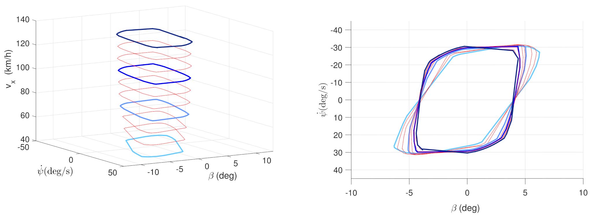
where is an experimentally defined parameter. Practically, the parameter of can be set to a smaller value than 1. The main role of the is to define the maximum allowed deviation between a linear and a nonlinear system during the reachability set calculation. Generally, it can be said that the increase in causes a smaller maximum deviation. More details can be found in [17]. Since some of the variables cannot be measured directly (or accurately), e.g., side-slip angle, a machine-learning technique is used to determine the stability of the vehicle during its operation, using only the signals that are available from the onboard system. Using (12), the reachability sets are computed by the convex hulls of the data points, which is illustrated in Figure 7. The convex hulls represent the boundaries of the stable regions in plane of and at different longitudinal velocities, . In the lateral control design, these reachability sets are used to compute the constraints of the states by which the stability of the vehicle can be guaranteed.
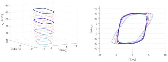
Figure 7.
Illustration of the reachability sets.
3.1.2. Evaluation of the Performances
In addition to stability, it is an important aspect to evaluate the network based on its performance in order to filter out those instances where the neural network provides poor results. This means that the output of the nominal system is compared to the output of the closed-loop (which contains the neural network) for the same input signal. The additional steering angle is computed by the neural network, which means that the goal is to evaluate the matching performance of the closed-loop. This classification is based on the following criterion:
where is a design parameter, which specifies the required accuracy between the nominal and measured yaw rates. During the determination of the parameter , the measurement noises can be taken into account. is the expected yaw rate, which can be computed from the nominal model (6) using the steering angle (), and is the measured yaw rate signal, which is provided by the CarMaker. Moreover, determines the bounds for the computation of this performance value. Practically, it can be chosen to a value of rad/s.
Basically, this criterion compares the expected and the measured yaw rate signals and categorizes the instances, using the deviation between them. The result of the categorization is two datasets: contains those instances in which the presented criterion (13) is satisfied, while the subset consists of the rest of the dataset.
3.2. Determination of the Neural Network Reliability
In this subsection, the reliability of the neural network is presented. Several methods can be found in the literature for the evaluation of the neural networks; see [23]. In this paper, the reliability analysis means that based on the measurable states of the vehicle, it is determined whether the network provides appropriate results or not. In this analysis process, the stability regions of the system are also taken into account indirectly.
The analysis is based on the previously calculated dataset, which is sorted into subsets. The goal of the reliability analysis is to examine, in a given operating range of the system, whether the neural network satisfies the requirements for stability and performance or not. Using this information, it is decided whether the additional term (output of the network) is added to the control input or not. The main role of this process is to increase performance in regions where the network gives appropriate results and avoid the cases where the results of the network may decrease the performance or stability.
During the reliability analysis of the neural network, all of the measurable data are used, which is detailed in Section 2. Firstly, the whole dataset is divided into two sets in terms of stability (), using (11) and (12). Secondly, two subsets are created, taking into account the performance of the closed-loop using the neural network . Furthermore, the performance and the stability of the system must be guaranteed at the same time. This means that the given data point is considered to be accepted if it satisfies both of the conditions (stability and performances). Based on the created subsets, the acceptable data can be determined, using the following expression:
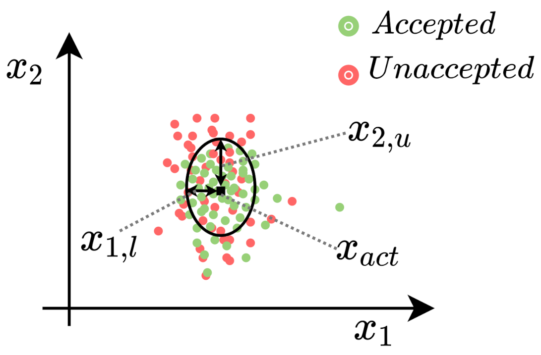
The whole reliability analysis is based on the created dataset described in (14). These subsets also contain the states of the vehicle. The analysis is performed in order to determine whether the neural network provides acceptable results at the given operating range of the system or not. During the computation of the reliability, the measurable states of the vehicle are used. Since, the states of the system can take arbitrary values with certain restrictions, during the computation of the reliability, a specified environment of the states is considered, , where gives the actual states of the system, and gives the lower and upper bounds of the actual states. This means that the reliability value is computed for the given region of the states, not for only one specific point. In Figure 8, an example is shown for a subset within which the reliability is computed (black line). In the figure, a lower bound for the first state () and an upper bound for the second state () is presented.

Figure 8.
Illustration of the subset for the analysis.
Each point in Figure 8 represents a measured data point. Using (14), all of the data points are evaluated and represented with green if the given point is acceptable in terms of stability and performance. Moreover, the unacceptable data are shown with red points. In the example, the system has two states, and the bounds are also shown with the black line. During the reliability analysis for the actual state, the probability of the acceptable results is determined using the Bayesian rule [32]:
where gives the probability of the acceptable results, if the states are . The goodness of the neural network can be given by term, which gives the rate of the acceptable data in the saved dataset. Finally, specifies a probability value that expresses how often the system is within the given operating range. The reliability of the neural network is computed by (15).
However, the determination of the optimal bounds () can be challenging for each state. For the determination of the optimal bounds, a clustering algorithm is used. The goal is to find the subsets within which the probability value does not change significantly. The subsets are calculated using the k-medoids clustering algorithm [33]. During the determination of the sets, the following cost function must be minimized:
where gives the center of the ith set, and is the jth point in the ith set. denotes the number of the elements in the given set, and N is the number of sets. The number of sets should be increased until the probabilities of any subset within a given set are nearly equal to the probability values calculated for the given set.
where defines the lower and upper bounds of the maximum deviation. The computation of the probabilities in real-time application cannot be achieved, due to the high amount of data. In order to meet this criterion, based on the results of (15), a piecewise linear function is determined:
where gives the ith subset, created by the clustering algorithm. Practically, this means that between two data points, the probability value is calculated, using interpolation.
Based on the proposed algorithm, the reliability of the neural network can be investigated. The reliability values contain the following three issues at the same time:
- The result of the network is not used in the range where its reliability is low (performances and stability).
- The result of the network is not used in the range where no training data are saved during the data collection process.
- Indirectly, sensor failure or an incorrect measurement sequence can be considered.
In summary, the goal is to determine the reliability of the neural network at the given operating point. In the cases when the reliability of the network is low, the additional steering angle is considered to be zero in order to avoid the instability and low performance of the system.
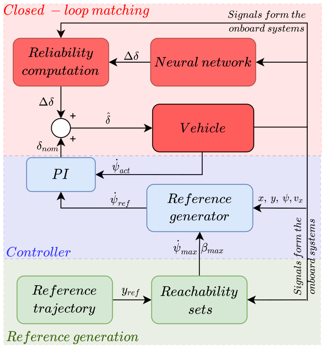
Finally, the whole algorithm is summarized in Figure 9. The additional steering angle is provided by the machine learning–based algorithm, by which the closed-loop matching is performed. Note that the neural network uses only those signals, which are available from the onboard system (see Section 2). Moreover, the checking of the additional control signal resulting from the machine learning algorithm is an important step to maintain stability. A data-driven approach is also applied to determine the reachability sets of the vehicle (), which is detailed in Section 3. During the reference signal generation, these sets are also taken into account. Furthermore, the reference signal is generated using only the nominal model of the system, which is detailed in Appendix A. Finally, the lateral controller is designed using only the nominal model of the nonlinear system.

Figure 9.
Structure of the algorithm.
4. Simulation Example
In this section, a comprehensive simulation example is presented to show the efficiency and the operation of the proposed control system. The whole simulation is made in CarMaker vehicle dynamics simulation software, in which the vehicle model is charged with nonlinearities. Firstly, the reliability computation for the neural network-based closed-loop matching process is tested in cases, when the vehicle is close to its physical limits. Secondly, a simulation example is presented for the reference trajectory tracking and compared the results for a nominal controller. In this case, the nominal controller means that the output of the neural network is set to zero.
4.1. Simulation Reliability of the Neural Network
During this simulation, the main goal is to show the effectiveness of the reliability computation algorithm. The main idea is to define a test scenario in which the neural network provides results with a low-performance level. This can be achieved, when the vehicle is driven close to its physical limits, and the nominal yaw rate value cannot be reached by the vehicle.
During the test scenario, the steering angle and the longitudinal velocity of the vehicle vary randomly in order to cover the whole stability region of the vehicle. In the first case, the computed, additional steering angle is added to the nominal steering angle during the whole simulation. Secondly, the additional steering angle is set to zero when the reliability of the neural network is low.
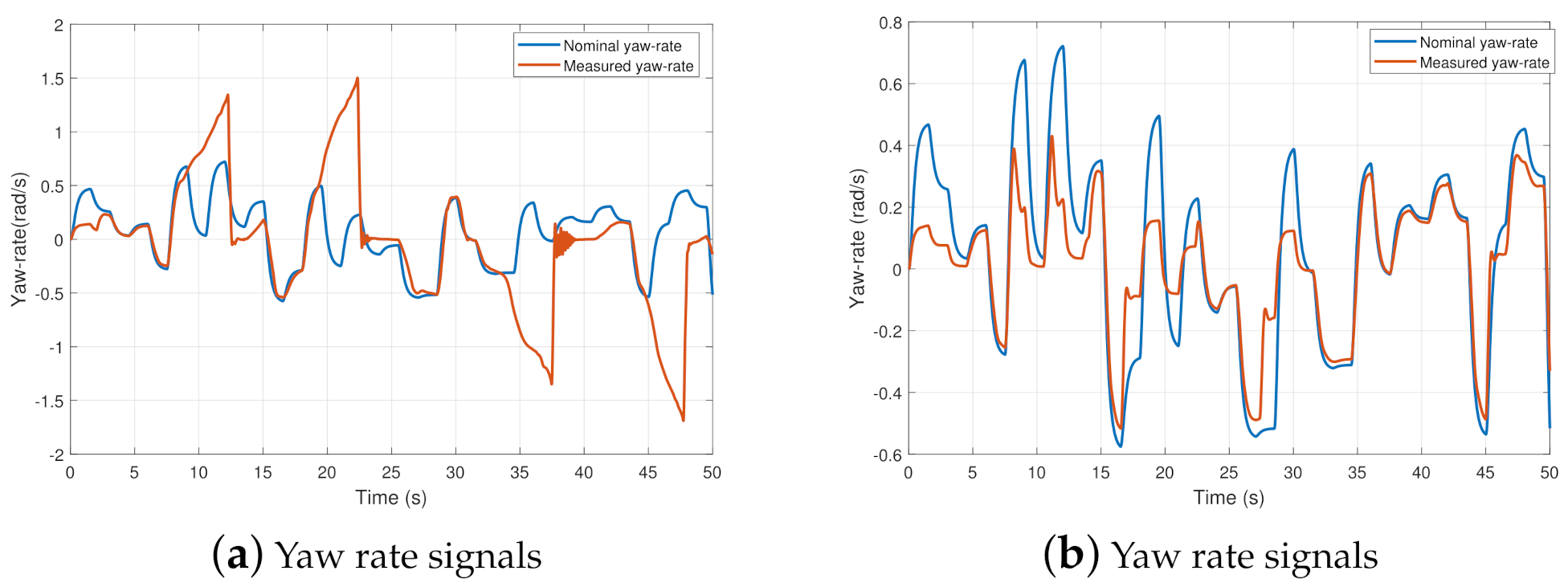
The results of the first simulation are presented in Figure 10a. Yaw rate values, measured from the simulation software, are presented with a red line, and the nominal yaw rates are represented with the blue line. It can be examined that the vehicle loses its stability in four regions during the simulation . However, within the other ranges of the test scenario, the yaw rate of the vehicle is nearly equal to the value, which is computed using the nominal model. This means that in these regions, the closed-loop matching process is successful but the loss of stability must be avoided.
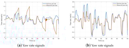
Figure 10.
Measured signal from simulation software and computed signal using the nominal model.
In Figure 10b, an example is shown in which the reliability computation is involved. This means that the additional steering angle is not added to the nominal steering angle when the computed reliability value is low. It can be seen that the model matching is not succeeded in the range . Nevertheless, the goal is to maintain stable motion of the vehicle in ranges where model matching cannot be performed.
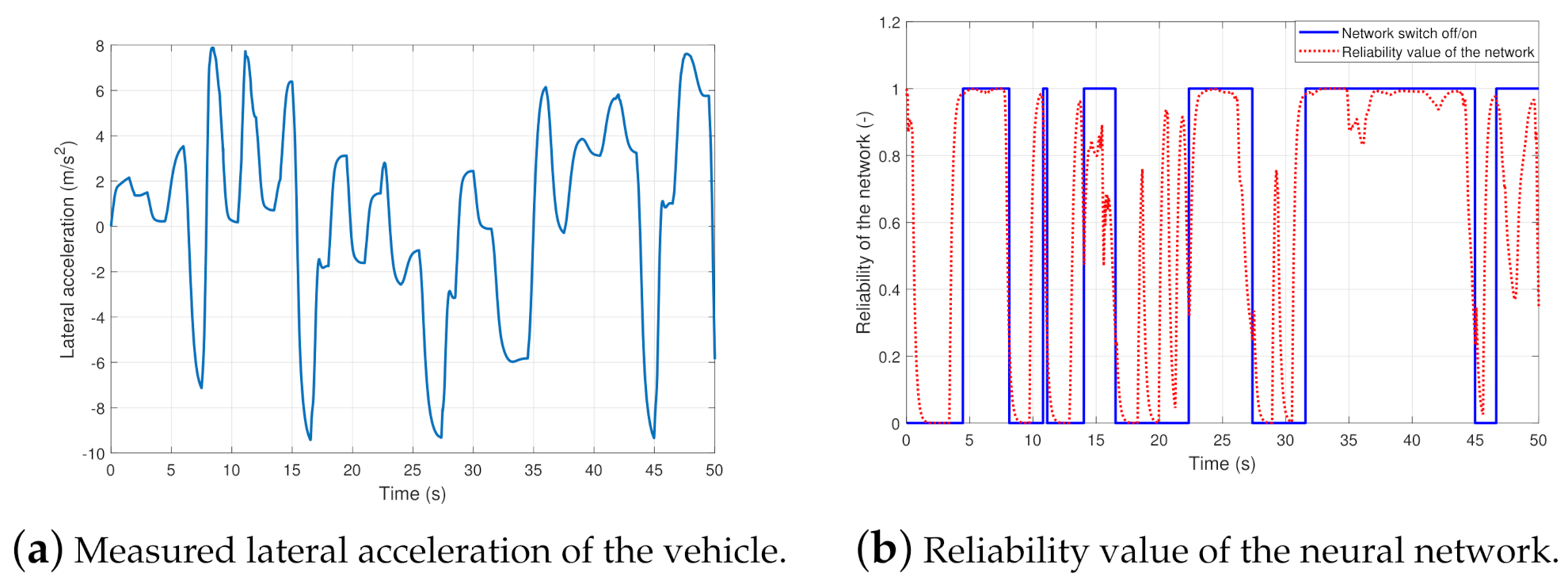
Generally, it can be said that the performance of the neural network decreases near the physical limits of the system, but the stability of the vehicle can be guaranteed. Moreover, in the regions where the reliability of the network is high, the performance can be increased significantly by adding the additional steering angle to the nominal value. In Figure 11a, the lateral accelerations are presented.
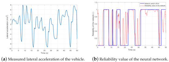
Figure 11.
Lateral acceleration and the computed reliability during the simulation.
Figure 11a depicts that the vehicle is near its physical limits, due to the high lateral acceleration values. Finally, in Figure 11b, the reliability of the neural network is presented. The red dashed line shows the actual value of the reliability. The blue line represents a discrete value, which gives the regions when the output of the network is considered to be zero (at the zero values).
4.2. Simulation for the Trajectory Tracking
In this subsection, a simulation is presented for trajectory tracking. During the calculation of the nominal transfer function, the longitudinal velocity is fixed at 100 km/h. Using the approximated parameters of the vehicle, and the constant velocity value, the transfer function of the nominal model is the following:
It is described above that the closed-loop matching is performed for the yaw rate of the vehicle. Based on the reference yaw rate generator, trajectory tracking is performed, which is presented in Appendix A. For the yaw rate tracking, a PI controller is designed using only the nominal model, which is described in (19). In the simulations, the vehicle must perform a complex test scenario in which it is driven along a predefined trajectory.
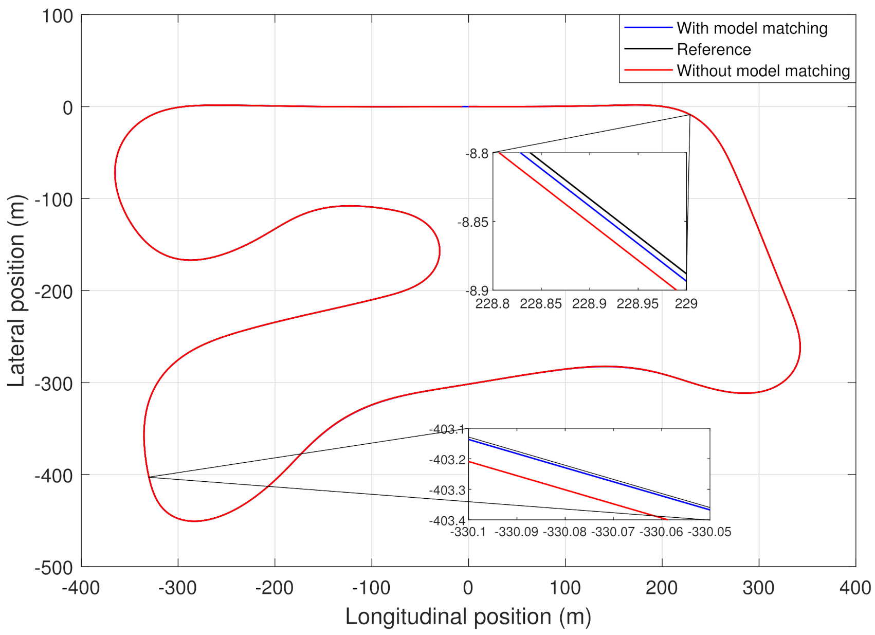
Figure 12 illustrates the reference trajectory of the vehicle, which is the Hockenheim racing circuit. Moreover, the measured lateral positions are presented. In the first case, the vehicle is controlled with the model-matching method. Secondly, a nominal control, without the matching algorithm, is used for the lateral control.
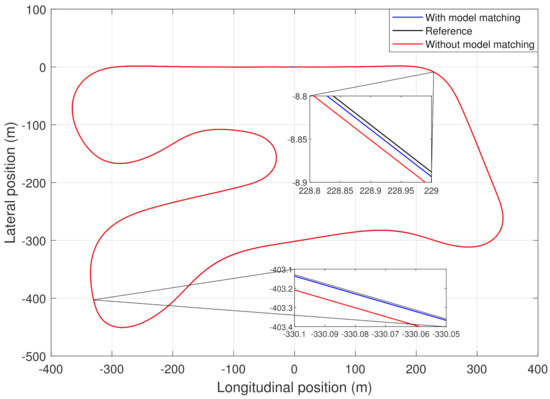
Figure 12.
Reference and the real trajectories of the vehicle.
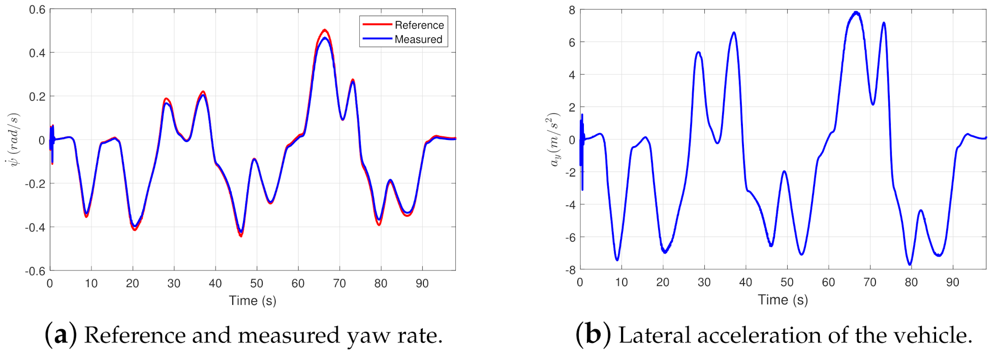
Figure 13a shows the tracking accuracy of the yaw rate signal, which is computed by the model-based reference signal generator. As it can be seen, the tracking of the reference value is appropriate, even at the high-velocity range. Figure 13b depicts the lateral accelerations for the vehicle. The maximum acceleration is about 8 m/s, which is close to the limitation of the vehicle. Nonetheless, the proposed control algorithm can guarantee the stability of the vehicle at that lateral acceleration.
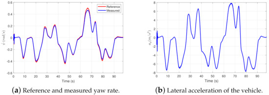
Figure 13.
Measured and calculated signals of the vehicle.
In Figure 14a, the results of the nominal controller are presented with blue, and the lateral error using the proposed method is shown with the red line. It can be concluded that the tracking error is also low in the nominal case but with the proposed method, this error can be further reduced.

Figure 14.
Tracing error and the reliability of the neural network.
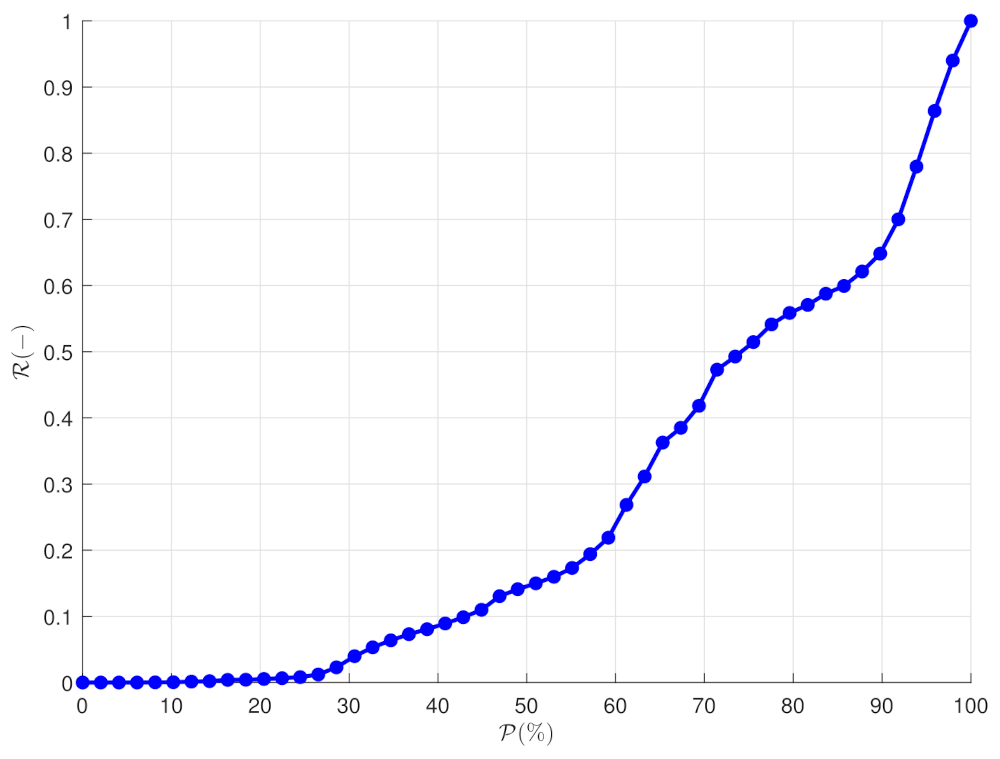
Figure 14b presents the reliability of the network during the simulation. At the beginning of the simulation, the reliability value decreases due to initialization problems. Nevertheless, in the rest of the simulation, the neural network operates with high reliability, even at high lateral acceleration values. Moreover, at ≈65 s of the simulation, the reliability of the network decreases; in Figure 13a, the highest yaw rate tracking error can be seen. This can be explained by the fact that the vehicle is close to its physical limits at the given operating point. In Figure 15, the error reduction rate is shown using the proposed method. The comparison is made for the data points in which the computed lateral errors are higher than 0.05 m and the lateral acceleration is above 0.5 m/s. It means that non-straight segments of the trajectory are considered, where the control system has a high impact on the tracking performance. The error reduction rate is computed as follows:
where gives the computed lateral error, using only the PI controller, and the lateral error using the proposed method is given by . Moreover, the percentage of the given reduction is computed as follows:
where N is the total number of data points and gives the number of data points, where the value of the rate is smaller than . The results of the analysis are presented in Figure 15.
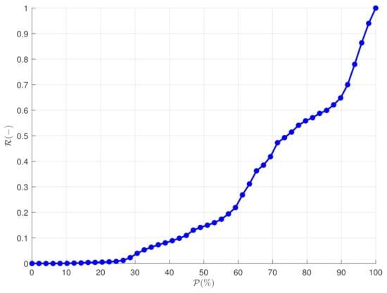
Figure 15.
Longitudinal velocity of the vehicle.
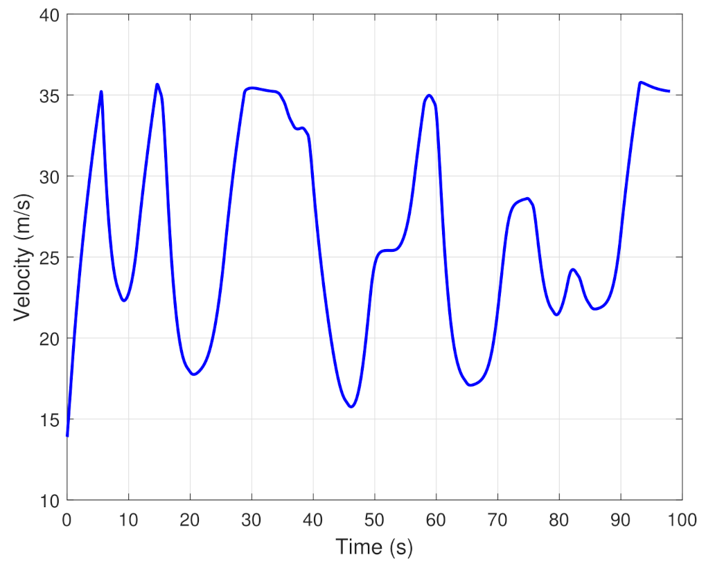
As the figure shows, the error decreases by more than in of the simulation. Moreover, the error value is reduced more than during ≈40% of the simulation time. It is important to note that in the case when the error value is already low for the nominal controller, no significant error reduction is expected. Because of these segments, the error reduction between and ≈25% is nearly 0. Finally, in Figure 16, the velocity of the vehicle is presented, which varies in a high range.
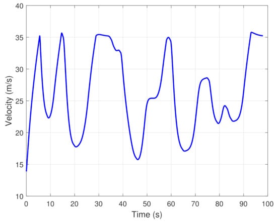
Figure 16.
Longitudinal velocity of the vehicle.
5. Conclusions
Sustainable urban transport can be promoted with the advent of autonomous vehicles. With accurate vehicle control, several effects of the transport system can be decreased, such as travel time, emission, fuel consumption. In this paper, a novel neural network–based model matching algorithm is proposed for highly automated vehicles, with which the accuracy of the tracking can be significantly increased. A neural network was applied to modify the lateral dynamics of the vehicle. The reliability of the network was checked, using a probability-based method. Using the calculated probability values, a piecewise linear function was determined with which the reliability of the network can be evaluated in real-time application. The modified nonlinear system was controlled with a simple PI controller, which was designed using the nominal model. Moreover, the reference signal was generated using the nominal model, which was extended with a result of the data-driven reachability sets.
The advantage of the proposed algorithm is that the actual parameters of the system are not known and the nonlinearities of the system are handled, using the model matching algorithm. Moreover, the whole control design can be made easily using only the nominal model. The accuracy of the yaw rate tracking was increased significantly in the scenario when the closed-loop matching algorithm was used. The operation and the efficiency of the proposed control strategy were demonstrated through a comprehensive simulation example in the simulation software, CarMaker.
The future challenge of the research is to take into account the impact of external disturbances and uncertainties (e.g., variation of the mass) on the closed-loop matching process, with which the robustness of the proposed method can be achieved. Moreover, a further challenge is to provide an extension of the method with which the training process of the neural network can be improved. For example, if the parameters of the vehicle during the operation are varied, the update of the neural network, e.g., through transfer learning, can be expected.
Author Contributions
Conceptualization, algorithms, software, T.H. and D.F.; methodology, T.H., D.F. and B.N.; supervision, P.G. All authors have read and agreed to the published version of the manuscript.
Funding
This research received no external funding.
Institutional Review Board Statement
Not applicable.
Informed Consent Statement
Not applicable.
Data Availability Statement
No data is available.
Acknowledgments
The research was supported by the Ministry of Innovation and Technology NRDI Office within the framework of the Autonomous Systems National Laboratory Program. The research was partially supported by the National Research, Development and Innovation Office (NKFIH) under OTKA Grant Agreement No. K 135512. The work of Tamás Hegedűs and Dániel Fényes have been supported by the ÚNKP-21-3 New National Excellence Program of the Ministry for Innovation and Technology from the source of the National Research, Development and Innovation Fund.
Conflicts of Interest
The authors declare no conflict of interest.
Appendix A. Determination of the Reference Signal
In the following, the model-based reference signal generation is presented. In this paper, the output of nonlinear is matched to the linear one with respect to the yaw rate. However, in many cases, the goal is to follow the predefined path during lateral control of the vehicle. In this section, the reference signal generation is presented in which the nominal model is taken into account. Using (1) and (2), a state-space representation can be determined in the following form:
where A and B are matrices, is the steering angle and the states are y , where gives the lateral velocity of the vehicle. However, during the reference signal generation, a discrete model is needed, which can be formed as follows:
where and , where is a sampling time. The main role of the model-based reference generation is to compute the reference yaw rate for the vehicle, which is tracked by the vehicle. The vehicle motion can be predicted, and the goal is to guarantee the tracking of the reference trajectory. Using (A2), the lateral position of the vehicle is predicted along the predefined time horizon (n):
In this case, the input vector of the system is defined as follows:
where gives the weight for the ith input signal. Using (A3) and (A4), the reference signal for the vehicle can be computed as follows:
where the reference trajectory is defined by the () vector and the actual states of the vehicle are given by . Moreover, gives the weights for the given time horizon.
During the computation, the reachability sets can be also taken into account, which serves the stability of the vehicle. This means that the states can be saturated, using the reachability sets. During the computation of the lateral error, the motion of the vehicle is predicted in order to decrease the lateral error during the tracking. Based on the actual states of the vehicle, the predicted error value can be computed as follows:
where denotes the length of the prediction and R is the reference position at the given state of the vehicle. In this paper, the value of the prediction is set to . Using the predicted error and (A5), the goal is to compute a yaw rate sequence with which the lateral error of the vehicle is zero at the end of the n horizon length.
References
- Das, S.; Sekar, A.; Chen, R.; Kim, H.C.; Wallington, T.J.; Williams, E. Impacts of Autonomous Vehicles on Consumers Time-Use Patterns. Challenges 2017, 8, 32. [Google Scholar] [CrossRef] [Green Version]
- Bissell, D.; Birtchnell, T.; Elliott, A.; Hsu, E.L. Autonomous automobilities: The social impacts of driverless vehicles. Curr. Sociol. 2020, 68, 116–134. [Google Scholar] [CrossRef]
- Treiber, M.; Kesting, A.; Thiemann, C. How Much Does Traffic Congestion Increase Fuel Consumption and Emissions? Applying Fuel Consumption Model to NGSIM Trajectory Data. In Proceedings of the 87th Annual Meeting of the Transportation Research Board, Washington, DC, USA, 13–17 January 2008. [Google Scholar]
- Barth, M.; Boriboonsomsin, K. Real-World Carbon Dioxide Impacts of Traffic Congestion. Transp. Res. Rec. 2008, 2058, 163–171. [Google Scholar] [CrossRef] [Green Version]
- Wadud, Z.; MacKenzie, D.; Leiby, P. Help or hindrance? The travel, energy and carbon impacts of highly automated vehicles. Transp. Res. Part Policy Pract. 2016, 86, 1–18. [Google Scholar] [CrossRef] [Green Version]
- Fan, R.; Jiao, J.; Ye, H.; Yu, Y.; Pitas, I.; Liu, M. Key Ingredients of Self-Driving Cars. arXiv 2019, arXiv:1906.02939. [Google Scholar]
- Isidori, A. Nonlinear Control Systems; Springer: Berlin/Heidelberg, Germany, 1995. [Google Scholar]
- Leith, D.J.; Leithead, W.E. Survey of gain-scheduling analysis and design. Taylor Fr. 2000, 73, 1001–1025. [Google Scholar] [CrossRef]
- Fenyes, D.; Nemeth, B.; Gaspar, P. LPV-based autonomous vehicle control using the results of big data analysis on lateral dynamics. In Proceedings of the 2020 American Control Conference (ACC), Denver, CO, USA, 1–3 July 2020; pp. 2250–2255. [Google Scholar]
- Tan, W.; Packard, A. Stability Region Analysis Using Polynomial and Composite Polynomial Lyapunov Functions and Sum-of-Squares Programming. IEEE Trans. Autom. Control 2008, 53, 565–571. [Google Scholar] [CrossRef]
- Jarvis-Wloszek, Z.; Feeley, R.; Tan, W.; Sun, K.; Packard, A. Some controls applications of sum of squares programming. In Proceedings of the 42nd IEEE International Conference on Decision and Control (IEEE Cat. No.03CH37475), Maui, HI, USA, 9–12 December 2003. [Google Scholar]
- Allgöwer, F.; Findeisen, R.; Nagy, Z. Nonlinear Model Predictive Control: From Theory to Application. J. Chin. Inst. Chem. Eng. 2004, 35, 299–315. [Google Scholar]
- Nemeth, B.; Gaspar, P.; Peni, T. Nonlinear analysis of vehicle control actuations based on controlled invariant sets. Int. J. Appl. Math. Comput. Sci. 2016, 26, 31–43. [Google Scholar] [CrossRef] [Green Version]
- Khalil, H.K. Nonlinear Systems, 3rd ed.; Prentice Hall: Hoboken, NJ, USA, 1997. [Google Scholar]
- Voosi, H. Nonlinear control of a quadrotor micro-UAV using feedback-linearization. In Proceedings of the 2009 IEEE International Conference on Mechatronics, Malaga, Spain, 14–17 April 2009; pp. 21–40. [Google Scholar]
- Pushkov, S.G. Inversion of Linear Systems on the Basis of State Space Realization. J. Comput. Syst. Sci. Int. 2017, 57, 7–17. [Google Scholar] [CrossRef]
- Fenyes, D.; Nemeth, B.; Gaspar, P. Impact of big data on the design of MPC control for autonomous vehicles. In Proceedings of the 2019 18th European Control Conference (ECC), Naples, Italy, 25–28 June 2019; pp. 4154–4159. [Google Scholar]
- Yesildirek, A.; Lewis, F.L. Feedback linearization using neural networks. Automatica 1995, 31, 1659–1664. [Google Scholar] [CrossRef]
- Pedro, J.O.; Dangor, M.; Dahunsir, O.; Alir, M.M. Dynamic neural network-based feedback linearization control of full-car suspensions using PSO. Appl. Soft Comput. 2018, 70, 723–736. [Google Scholar] [CrossRef]
- John, S.; Pedroi, J. Neural Network-Based Adaptive Feedback Linearization Control of Antilock Braking System. Int. J. Artif. Intell. 2013, 10, 21–40. [Google Scholar]
- Westenbroek, T.; Fridovich-Keil, D.; Mazumdar, E.; Arora, S.; Prabhu, V.; Sastry, S.S.; Tomlin, C.J. Feedback Linearization for Unknown Systems via Reinforcement Learning. arXiv 2020, arXiv:1910.13272. [Google Scholar]
- Castaneda, F.; Wulfman, M.; Agrawal, A.; Westenbroek, T.; Tomlin, C.J.; Sastry, S.S.; Sreenath, K. Improving Input-Output Linearizing Controllers for Bipedal Robots via Reinforcement Learning. arXiv 2020, arXiv:2004.07276. [Google Scholar]
- Burton, R.M.; Faris, W.G. Reliable evaluation of neural networks. Neural Netw. 1991, 4, 411–415. [Google Scholar] [CrossRef]
- Rajamani, R. Vehicle Dynamics and Control; Springer: Berlin/Heidelberg, Germany, 2005. [Google Scholar]
- Mortazavizadeh, S.A.; Ghaderi, A.; Ebrahimi, M.; Hajian, M. Recent Developments in the Vehicle Steer-by-Wire System. IEEE Trans. Transp. Electrif. 2020, 6, 1226–1235. [Google Scholar] [CrossRef]
- Shamash, Y. Construction of the inverse of linear time-invariant multivariable systems. Int. J. Syst. Sci. 1975, 6, 733–740. [Google Scholar] [CrossRef]
- Devasia, S.; Paden, B. Stable inversion for nonlinear nonminimum-phase time-varying systems. IEEE Trans. Autom. Control 1998, 43, 283–288. [Google Scholar] [CrossRef] [Green Version]
- Malinen, J. Tustin’s method for final state approximation of conservative dynamical systems. IFAC Proc. Vol. 2011, 44, 4564–4569. [Google Scholar] [CrossRef]
- Demut, H.; Hagan, M.; Beale, M. Neural Network Design; PWS Publishing Co.: Boston, MA, USA, 1997. [Google Scholar]
- The MathWorks Inc. Deep Learning Toolbox; The MathWorks Inc.: Natick, MA, USA, 2018. [Google Scholar]
- Boyd, S.; Ghaoui, L.E.; Feron, E.; Balakrishnan, V. Linear Matrix Inequalities in System and Control Theory; Society for Industrial and Applied Mathematics: Philadelphia, PA, USA, 1997. [Google Scholar]
- Bolstad, W.M. Introduction to Bayesian Statistics; John Wiley and Sons, Ltd.: Hoboken, NJ, USA, 2007. [Google Scholar]
- Schubert, E.; Rousseeuw, P.J. Faster k-Medoids Clustering: Improving the PAM, CLARA, and CLARANS Algorithms. In Lecture Notes in Computer Science; Springer: Cham, Germany, 2019; pp. 171–187. [Google Scholar]


Publisher’s Note: MDPI stays neutral with regard to jurisdictional claims in published maps and institutional affiliations. |
© 2021 by the authors. Licensee MDPI, Basel, Switzerland. This article is an open access article distributed under the terms and conditions of the Creative Commons Attribution (CC BY) license (https://creativecommons.org/licenses/by/4.0/).