Abstract
The impacts of future climate changes on watershed hydrochemical processes were assessed based on the newest Shared Socioeconomic Pathways (SSP) scenarios in Coupled Model Intercomparison Project Phase 6 (CMIP6) in the Tianhe River in the middle area of China. The monthly spatial downscaled outputs of General Circulation Models (GCMs) were used, and a new Python procedure was developed to batch pick up site-scale climate change information. A combined modeling approach was proposed to estimate the responses of the streamflow and Total Dissolved Nitrogen (TDN) fluxes to four climate change scenarios during four future periods. The Long Ashton Research Station Weather Generator (LARS-WG) was used to generate synthetic daily weather series, which were further used in the Regional Nutrient Management (ReNuMa) model for scenario analyses of watershed hydrochemical process responses. The results showed that there would be 2–3% decreases in annual streamflow by the end of this century for most scenarios except SSP 1-26. More streamflow is expected in the summer months, responding to most climate change scenarios. The annual TDN fluxes would continue to increase in the future under the uncontrolled climate scenarios, with more non-point source contributions during the high-flow periods in the summer. The intensities of the TDN flux increasing under the emission-controlled climate scenarios would be relatively moderate, with a turning point around the 2070s, indicating that positive climate policies could be effective for mitigating the impacts of future climate changes on watershed hydrochemical processes.
1. Introduction
Global climate change has affected the Earth system [1,2,3], and it will continue to do so, judging from current trends [4,5]. Among its significant impacts are those on watershed hydrochemical processes [6,7,8]. The expected temperature changes are likely to alter the water cycle across global to regional scales and modify watershed hydrology by increasing evapotranspiration [9] and evaporation [10], lowering soil moisture [11], reducing snow cover and generating earlier snowmelt [12]. In addition, watershed hydrochemical processes could also be altered by changes in precipitation, both in terms of absolute yields and temporal and spatial distributions, which are directly related to streamflow and non-point source flux [13,14]. Understanding the response of watershed streamflow and pollution load to climate change has important implications for the local management of water security, water quality, and ecosystem sustainability [15,16]. A modeling approach is often considered to be a useful tool to quantitatively estimate the impacts of projected climate changes on watershed hydrochemical processes based on scenario analyses [17,18]. The main subject of the article is to apply a multi-model approach to estimate the impacts of climate changes on watershed streamflow and non-point source flux.
Downscaled outputs of General Circulation Models (GCMs) have been widely used to drive watershed models to estimate the responses of watershed hydrological or hydrochemical processes to projections of climate change [19,20]. The Coupled Model Intercomparison Project (CMIP) was organized by the Working Group on Coupled Modeling (WGCM) in 1995 and developed in phases with numerous collaborations. The most important of these collaborations was with the US Department of Energy (DOE) Program for Climate Model Diagnosis and Intercomparison (PCMDI). The CMIP is a collaborative framework to make the model intercomparison data available to other scientists as the standard experimental protocol of climate change scenarios for international scientists to analyze different GCMs in an equivalent way and facilitate further applications. Since 2016, a new set of emissions scenarios driven by different socioeconomic assumptions, called Shared Socioeconomic Pathways (SSPs), has been developed by the energy modeling community and selected as new scenarios in CMIP6 to drive GCMs for further analysis [21,22], such as the upcoming 2021 Intergovernmental Panel on Climate Change (IPCC) sixth assessment report (AR6). Datasets from the new generation of GCMs based on CMIP6 scenarios are gradually being released [23], representing new characteristics in the frequency and intensity of climate change [24,25,26]. It is of great interest to both researchers and decision makers to estimate how the watershed streamflow and water quality will change under the new emission scenarios in the future. However, previous studies were mainly carried out based on CMIP5 scenarios [27,28], and studies based on the state-of-the-art scenarios of CMIP6 are pending [29,30]. In this subject, we hope to establish a feasible technical framework to provide insight into climate change impacts on the watershed hydrochemical processes under CMIP6 scenarios with a multi-model approach.
The resolutions of global raster maps from GCM outputs are generally too low to be directly used in watershed models, which often require at least daily weather data at the site-scale resolution. However, as a critical issue for CMIP6 scenario application [31], reanalysis of the original GCM outputs for resolution refinement is pending and still not available for most GCMs’ daily outputs in the most areas due to its high computational complexity. It is a great challenge to bridge the gap between GCM outputs and watershed model demands [32,33], and practical downscaling analysis is an effective technical approach to address this issue [34,35]. There are generally two technical paths to downscale the GCM outputs: dynamic downscaling and statistical downscaling. The dynamic downscaling methods mainly use Regional Climate Models (RCMs) driven based on GCM outputs for detailed re-analyses [36,37], which need remarkable computational resources. Statistical downscaling methods mainly use various Markov chains, spatial interpolation, and machine learning methods, such as Convolutional Neural Networks (CNNs) for spatial downscaling and the Weather Generator (WG) model for time downscaling [38,39,40]. The WG model has relatively simple operation and low computational cost to generate site scale synthetic daily weather series suitable for watershed model applications. It has been widely used in estimating the responses of watershed hydrological or hydrochemical processes to various climate changes of CMIP5 scenarios by estimating watershed-scale climate variables consistent with the GCM outputs [41,42,43]. It is a feasible approach to estimate watershed responses to CMIP6 scenarios by developing a framework based on a suitable WG model combined with a watershed hydrology model.
In this study, we propose a combined modeling approach to estimate climate change impacts on a watershed under CMIP6 scenarios. As a tributary of the Hanjiang River in China, the Tianhe River was used as a study case. The changes of streamflow and total dissolved nitrogen (TDN) fluxes at the estuary of the Tianhe River as the watershed outlet were estimated. The results show that both watershed hydrological and hydrochemical processes would be changed under SSP scenarios in the future, including more TDN yields, different monthly load distributions and source apportionment, and increasing risks of extreme events. More response estimations based on SSP scenarios of CMIP6 in other watersheds with different weather conditions are expected, and the modeling approach proposed in this study can be adopted as an alternative.
2. Materials and Methods
2.1. Study Area and Data Source
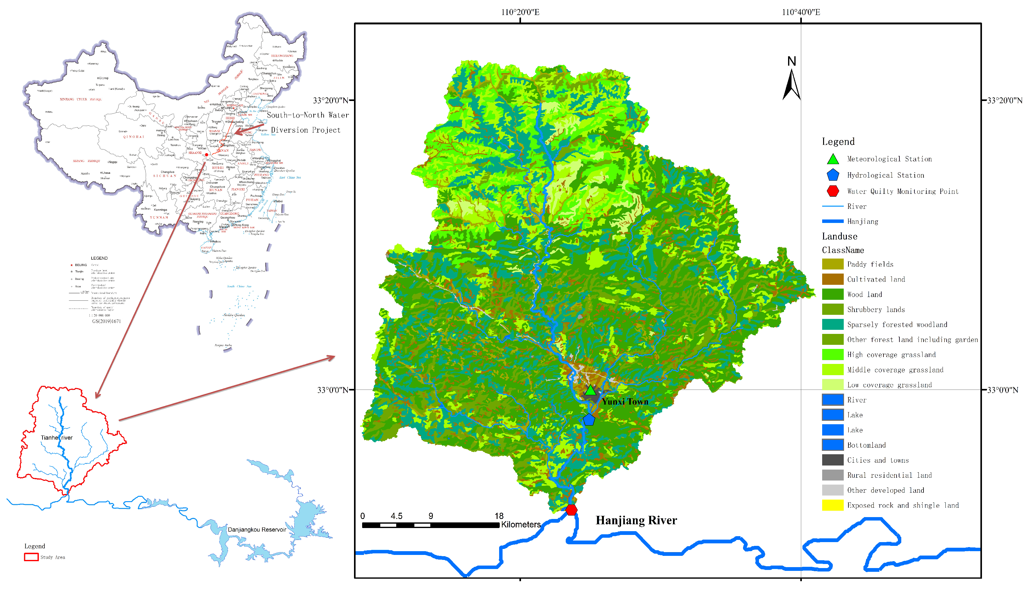
This study was conducted in the Tianhe River watershed, located in the middle area of China (Figure 1). The Tianhe River originates from the eastern side of Taiping Mountain in Shaanxi Province and drains into the Hanjiang River in Hubei Province. The Hanjiang River is the main water source of Danjiangkou Reservoir. Danjiangkou Reservoir is the source of water for extraction by China’s South-to-North Water Diversion Project. It has a 290.5 × 10⁸ m3 maximum storage capacity and 394.8 × 10⁸ m3 mean annual inflow, indicating great socioeconomic value. The Tianhe River is the last large tributary of the Hanjiang River before being injected into the Danjiangkou Reservoir. Due to the active agricultural planting behavior in the upstream and the septic system discharge from residents in the downstream town, the TDN concentration of the Tianhe River is generally at a relatively high level, leading to the risk of eutrophication in the Danjiangkou Reservoir. In addition, residents living in the downstream town face the risk of flooding during the summer. Thus, it is of significance to estimate the possible changes of the streamflow and TDN fluxes in the Tianhe River caused by climate change in the future.

Figure 1.
Location of the study area.
The watershed area located above the estuary of the Tianhe River was set as the study area, approximately 1702 km2. It is dominated by natural land with 63.4% forest and 24.3% grassland cover, mainly distributed in the upstream area. There is considerable cultivated land in the downstream area, accounting for 11.2% of the total watershed area. Elevations range from 147 m to 1590 m, and the average annual precipitation and temperature of this area are 810.2 mm and 12.5 °C, respectively (Figure 2). Yunxi town is located in the downstream area of the study’s watershed, with a population of about 505,000. There is one water quality monitoring station, one hydrological station, and one meteorological station lying in the study’s watershed. The historical data from the meteorological station provide weather data for GCM downscaling and watershed hydrochemical modeling. The historical data from the hydrological station provide streamflow data for transport parameter estimation of the ReNuMa model. The historical data from the water quality monitoring station provide TDN data for nutrient parameter estimation of the ReNuMa model. The sources of the original data used in this study are summarized in Table 1.
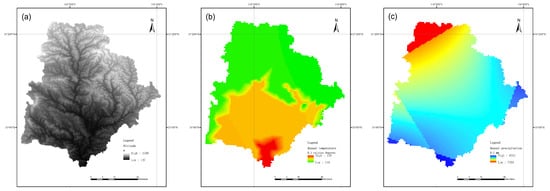
Figure 2.
Spatial attributes of the study area (statistics since 1980). (a) The spatial distribution of elevation. (b) The spatial distribution of temperature. (c) The spatial distribution of precipitation.

Table 1.
Summary of the original input data source.
2.2. Overview of Methodology
In this study, we propose a combined modeling approach to estimate climate change impacts on a watershed under CMIP6 scenarios. The WG model of the Long Ashton Research Station Weather Generator (LARS-WG) was employed to provide site-scale daily temperatures and precipitations suitable for watershed model application. LARS-WG is an effective time downscaling tool that can generate synthetic daily weather series based on monthly climate change estimations. This means that just monthly downscaling analysis of the original GCM outputs can satisfy the modeling demand of LARS-WG to address the time disaster caused by complex computation. The monthly downscaled dataset is already available in some public databases. Global monthly 2.5-min raster maps, downscaled with WorldClim v2.1 based on the original GCM outputs, were used to provide high-resolution future climate data under various SSP-CMIP6 scenarios in different periods [44]. A Python procedure was developed to extract site-specific climate variables for the target watershed in batch mode for four future periods under four different SSP scenarios from seven available GCMs. An ensemble approach was adopted by averaging the values of the estimated climate variables from multi-GCM outputs to avoid uncertainty from one single GCM. The changes in the monthly climate variables in different SSP scenarios and future periods were calculated to build several user-defined scenario files, which were used to update the parameters of LARS-WG to generate synthetic daily weather data representing various scenarios and periods for further application in the watershed model. Regional Nutrient Management (ReNuMa) was employed as a watershed model tool to estimate the watershed hydrological and hydrochemical processes, including the current status and various possible responses to climate changes by using LARS-WG outputs. The general methodology diagram is shown in Figure 3.
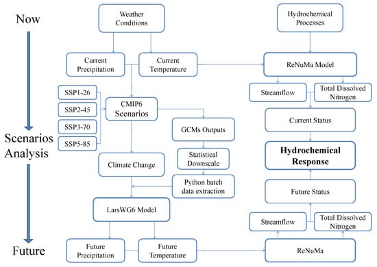
Figure 3.
The general flow chart of the methodology. The abbreviation ReNuMa stands for the Regional Nutrient Management model. The abbreviation LARS-WG 6 means the Long Ashton Research Station Weather Generator Version 6.
2.3. Watershed Hydrochemical Modeling
Regional Nutrient Management (ReNuMa) was used to model the watershed hydrochemical process for streamflow and TDN flux estimations. ReNuMa is a semi-distributed watershed model as a derivative of the Generalized Watershed Loading Function (GWLF) [45] with the Net Anthropogenic Nitrogen Inputs (NANI) framework, which is an accounting methodology for calculating the nitrogen concentrations of the discharge from different land use areas based on the estimations of the net anthropogenic nitrogen inputs across watershed boundaries [46]. It has been widely applied to estimate the yields and source apportionments of watershed streamflows and pollution fluxes [47], as well as for various scenario analyses of watershed responses to a changed environment, such as best management practice implementation [48,49] and climate or land use cover changes [18,50]. The ReNuMa model can provide reliable monthly to annual estimations in several hundred to a thousand square kilometer watersheds with moderate data requirements, which is suitable for the modeling demands of this study.
ReNuMa applications generally include parameter estimation and scenario analysis. Due to the limitations of available historical data, the periods of observed data of streamflow and water quality for parameter estimation do not overlap. It conforms to the model application specifications, as the transport parameters and nutrient parameters were estimated sequentially. The nutrient-related parameters of ReNuMa are estimated only after the hydrological parameters are established by calibration. The historical hydrological data of the observed monthly streamflow at the Jia-Jia-Fang Hydrological Station from 2009 to 2012 were used to calibrate the transport parameters for streamflow estimation, and historical data from 2013 to 2015 were reserved for testing the validity of the model with the calibrated parameters. The nutrient parameters for TDN estimation were calibrated based on the historical monthly water quality data at Tianhe-Estuary Monitoring Point from 2012 to 2015 and validated with observed data in 2016 and 2018. The Nash–Sutcliff coefficient (R2NS) and coefficient of determination (r2) are used as statistics to measure the model’s accuracy. The nonlinear least square method was used for model calibration with the Solver macro add-in procedure embedded in ReNuMa’s Excel platform [51]. Two additional algorithms of the segment function and leakage transport approach based on the previous study [52] were used. The former used variable recession and seepage coefficients based on saturated zone soil moistures instead of the original fixed coefficients for better specification of the proportions of groundwater added to the stream and lost to the deep aquifer. The latter establishes an additional pathway for water infiltration from an unsaturated zone to a saturated zone, regardless of whether the unsaturated zone soil moistures exceed the moisture storage capacity or not. These new algorithms could refine the model groundwater framework and achieve better estimations of groundwater yields during low-flow periods. The calibrated ReNuMa was then used to estimate the watershed responses to alternative climate scenarios by updating the weather input data with downscaled synthetic daily series, as described below.
2.4. Downscaling Analysis
The Long Ashton Research Station Weather Generator (LARS-WG) was used as the time-downscaling tool for future climate changes in this study. It is a stochastic weather generator that can generate synthetic daily weather data based on the lengths of wet and dry day series and the semi-empirical distributions of weather factor values to represent current and various projected future climate statuses [53]. The LARS-WG has been widely used for watershed response estimations to climate changes by linking its output to various watershed hydrochemical models [54,55].
In this study, the newest version of LARS-WG6 was used, and 63 years of observed daily weather data from 1957 to 2019 from the Meteorological Station of Xun-Xi were analyzed to assess the statistical characteristics of critical weather factors in the study area in order to calibrate the model parameters. Then, 63 years of synthetic daily weather data were generated based on the calibrated parameters and compared with the observed data to validate the parameters. Three statistical tests were conducted to test the consistencies between the modeled and observed data for different weather factors. The Kolmogorov–Smirnov (K–S) test was performed for the significance test of the daily minimum temperature distributions, daily maximum temperature distributions, seasonal wet/dry series distributions, and daily precipitation distributions. In addition, the consistencies of the monthly mean of precipitation, monthly mean of the daily maximum temperature, and monthly mean of the daily minimum temperature were tested by the t-test, and the monthly variances of precipitation were tested by the F-test. After the model performance has been approved, synthetic daily weather data that represent various changed climatic statues can be generated by updating the calibrated and validated model parameters based on scenario files. However, the scenario analysis module in the current LARS-WG6 was developed based on CMIP5 so that it does not reflect changes in the statistical characteristics of weather factors under CMIP6 SSP scenarios to update the model parameters. Thus, a series of user-defined scenario files for LARS-WG6 were built to update the model parameters to reflect the responses of critical weather factors to climate changes in different future periods under different CMIP6 SSP scenarios.
The global 2.5-min raster maps in the WorldClim dataset were used as climatic input data to build the LARS-WG6 scenario files, which were downscaled from the original GCM outputs to present averages of the monthly temperature and precipitation values over 20-year periods for various CMIP6 SSP scenarios. Seven available GCM outputs were considered, including BCC-CSM2-MR, CNRM-CM6-1, CNRM-ESM2-1, CanESM5, IPSL-CM6A-LR, MIROC-ES2L, and MIROC6. A Python batch procedure was developed to select the raster values of the study area for each of the GCMs included. An ensemble approach was achieved based on the averages of multiple GCM outputs to account for the scenario files [56]. More details about the GCMs and ensembles are provided in the Supplementary Materials. Based on these scenario files, various synthetic daily weather series were generated by using LARS-WG6 for further applications in ReNuMa to estimate the impacts of future climate changes on watershed hydrochemical processes, as described below.
2.5. Scenario Descriptions
The impacts of future climate changes under four climate change scenarios in four future periods were estimated. The state-of-the-art climate change scenarios of the Shared Socioeconomic Pathways (SSPs) proposed by the energy modeling community for CMIP6 [22] have been used by many modeling groups to drive different climate models to estimate how the global climate may change under various future emission scenarios. Four SSP scenarios available in the WorldClim dataset were considered in this subject, including SSP1-26, SSP 2-45, SSP 3-70, and SSP 5-85. The scenarios of SSP1-26, SSP 2-45, and SSP 5-85 can be seen as new versions of the scenarios of RCP26, RCP45, and RCP85 in AR5/CMIP5, which have similar end-of-century radiative forcing levels but different emissions pathways and mixes of CO2 and non-CO2 emissions. SSP 3-70 is a new scenario added in CMIP6. It lies in the middle of the range of baseline outcomes produced by energy system models. Generally speaking, SSP1-26 and SSP 2-45 represent a controlled world that rapidly reduces emissions for the situations of limited warming to below 2 °C and around 3 °C by 2100, respectively. SSP5-8.5 and SSP3-7.0 represent a world that fails to enact any climate policies for the situations of the worst case and the middle of the road, respectively.
The possible climate changes in four future periods were considered, including the 2030s (2021–2040), 2050s (2041–2060), 2070s (2061–2080), and 2090s (2081–2100). Each future period climate raster dataset was based on the time averages of 20 years of downscaled GCM outputs. For each month in each future period under each SSP scenario, the changes in monthly temperature and precipitation in the study area from each GCM output were averaged and used to update the model parameters to construct the respective scenario files for LARS-WG6 to generate 20 years of synthetic daily weather data, which were further used in ReNuMa for scenario analyses of the watershed hydrochemical process. All the parameters of ReNuMa are constant, based on the assumption that there is no change in the inputs of pollution to the watershed resulting from local human activities so that only the impacts of climate changes are estimated. The annual and monthly streamflow and TDN fluxes at the watershed outlet were estimated for each scenario and future period, which were further compared with the results in the current status for response estimation. The impacts of climate changes on the watershed hydrochemical processes were discussed for local decision-making support, including possible water source yields, extreme event probabilities of flood and eutrophication risks, and changes in pollution source apportionment, as described in Section 3 below.
3. Results and Discussion
3.1. Results of the LARS-WG
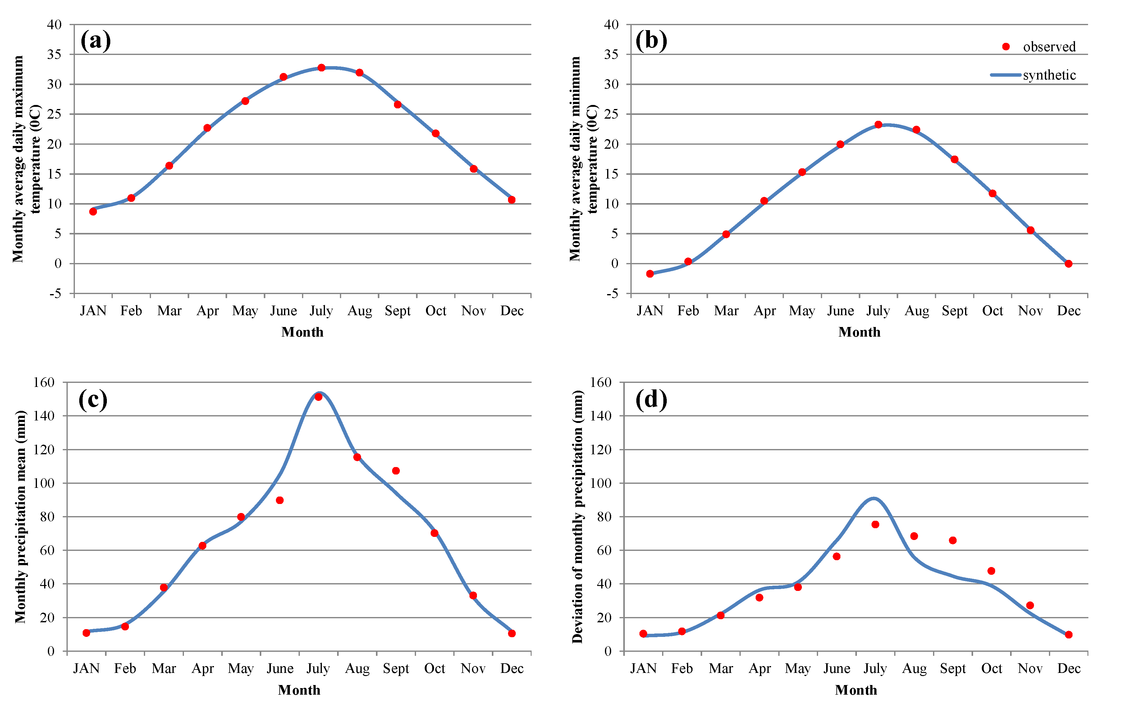
The outputs of the LARS-WG compared with the observed values are shown in Figure 4. There was generally great similarity between the observed and modeled values of the monthly means of the daily maximum and minimum temperatures and monthly precipitation totals. The results were much better for temperature than precipitation, which is consistent with the results of other similar studies [57,58]. The temperature was more regularity affected by the season, but the occurrence of precipitation behavior was more uncertain and hard to be totally simulated. The results of the K-S tests show that there was no significant difference between the distributions of the daily observed and modeled series for all weather factors. The t-test and F-test results show that the means and variances of the monthly observed series and synthetic series were in good agreement, if a little poorer than the corresponding daily outputs, and comparable with the level of agreement in other model applications [56,59,60]. Most monthly results had no significant differences between the observed and modeled values at the 5% significance level, except the F-test of monthly precipitation variance in September. The modeling performance file and parameter file of the LARS-WG are provided in the Supplementary Materials. The calibrated and validated LARS-WG model was thus judged to be acceptable to generate synthetic weather series based on projected climate scenarios.
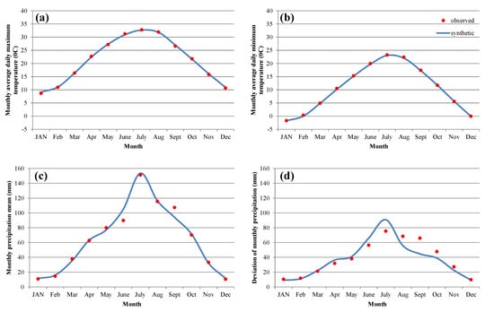
Figure 4.
Comparisons of observed and modeled values of precipitation and temperature from the Long Ashton Research Station Weather Generator (LARS-WG). (a) The mean daily maximum temperature for each month. (b) The mean daily minimum temperature for each month. (c) The monthly precipitation for each month. (d) The deviation of monthly precipitation for each month.
The scenario files of the LARS-WG contained a series of user-defined parameters based on the ensembles of downscaled GCM outputs. For each SSP scenario in each future period, the changes in precipitation and maximum and minimum temperatures in each month were summarized with the Python batch procedure to create the corresponding scenario file of the LARS-WG. For each scenario file, 20 years of daily synthetic weather series of the precipitation, maximum temperature, and minimum temperature were generated by the LARS-WG model. All the scenario files and corresponding synthetic weather data can be found in the Supplementary Materials. These synthetic daily series were used as the input weather data of the ReNuMa model for scenario analyses. The average of the daily maximum and minimum temperatures was used as the input of the daily temperature data for ReNuMa.
3.2. Results of ReNuMa for Streamflow and TDN Flux: Calibration and Validation
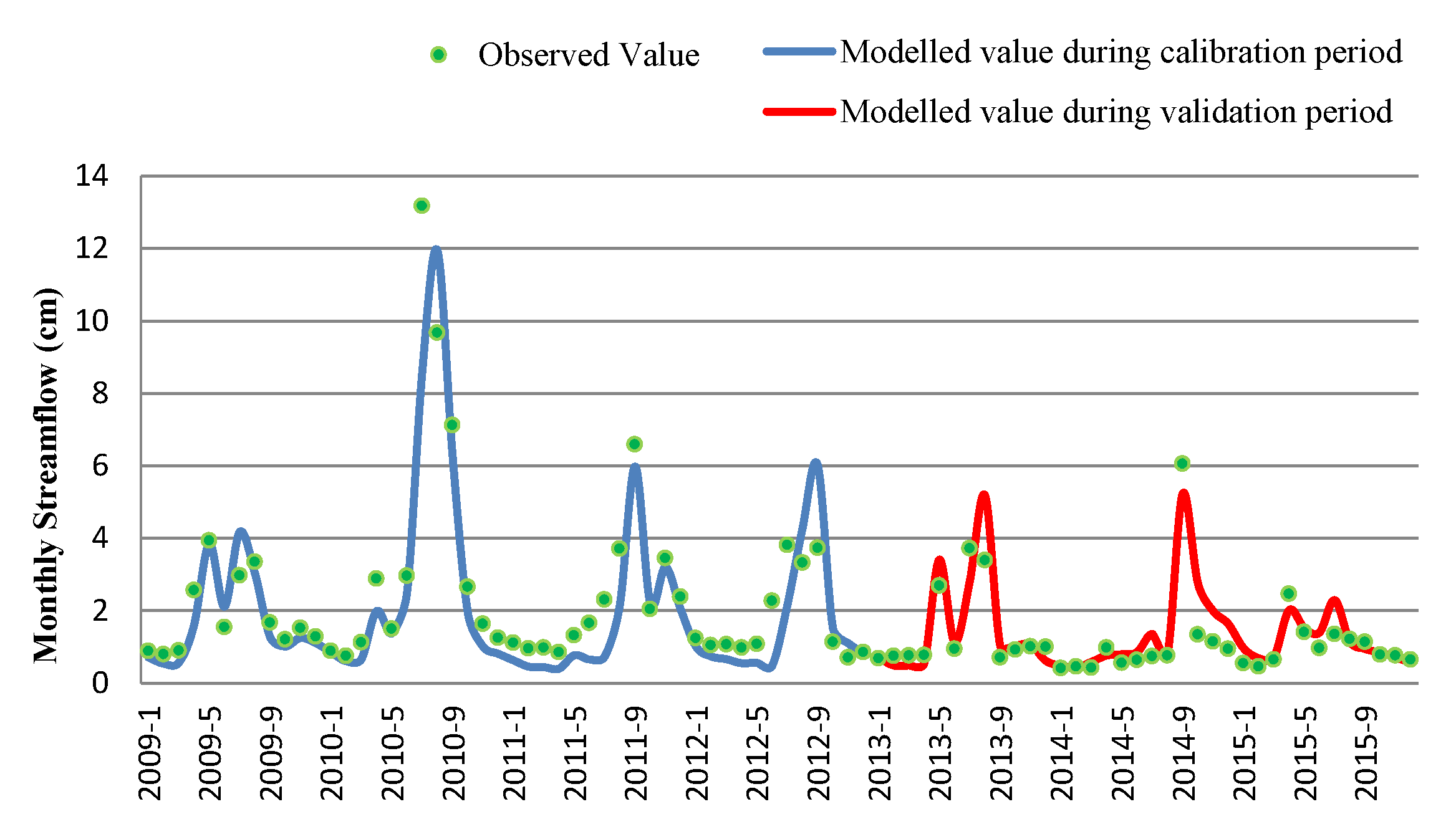
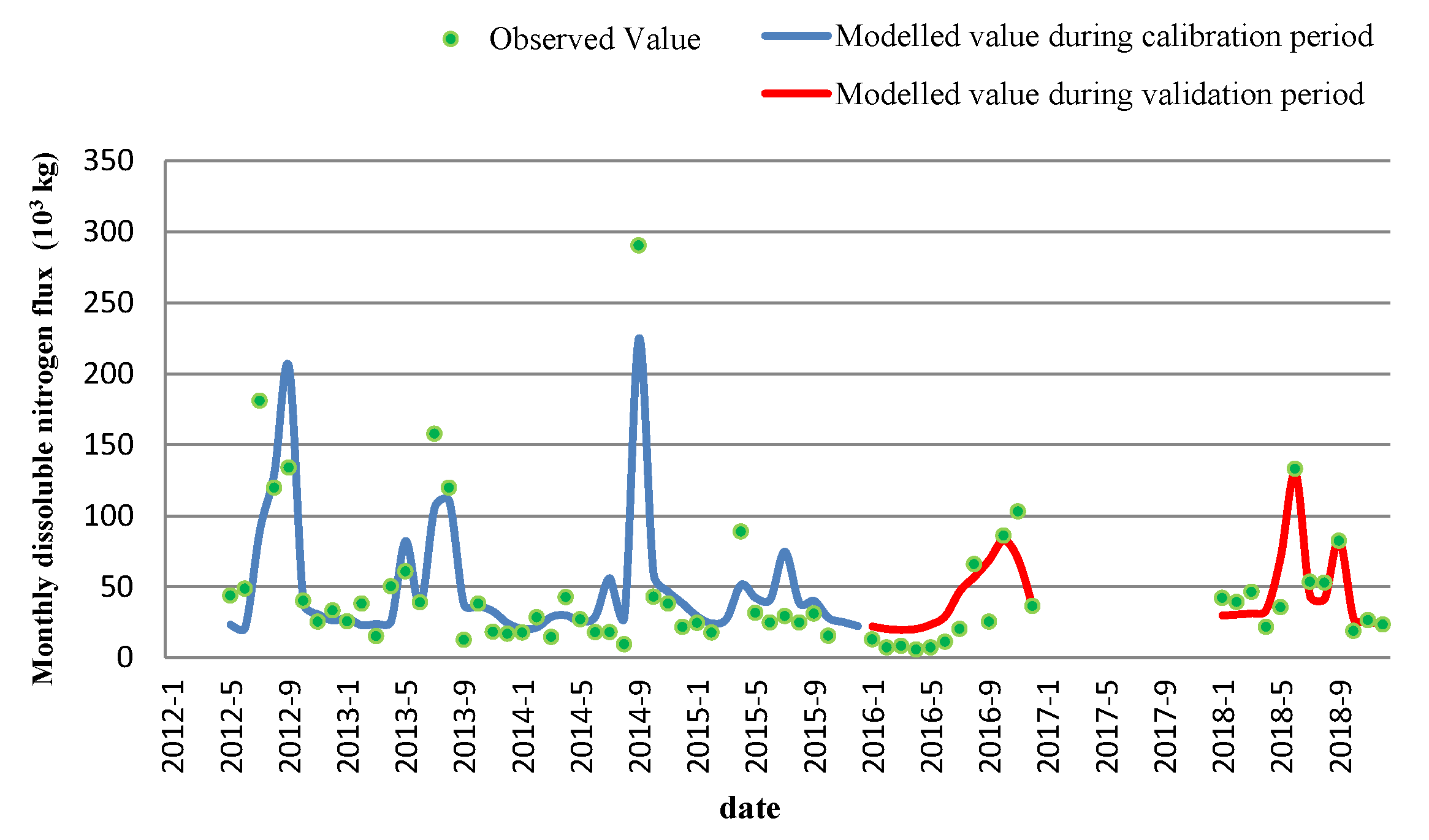
The time series of the monthly modeling streamflow and TDN compared with the observed data are shown in Figure 5 and Figure 6. The results showed relatively good agreement, based on the goodness of fit of the observed and modeled streamflow and TDN flux in this study area. The observed TDN in 2017 is missing due to available data limitations. However, benefiting from the flexible data demands of ReNuMa, it was feasible to use discontinuous observation for calibration and verification. The R2NS and r2 of the streamflow estimation were 0.800 and 0.828 in the calibration period and 0.753 and 0.796 in the validation period, respectively. The modeling accuracy for TDN flux was somewhat lower than that for the streamflow, which is consistent with previous studies [48,49]; the R2NS and r2 values for TDN flux estimation for the calibration period were 0.748 and 0.751, respectively. For the validation period, the R2NS was 0.716, and the r2 was 0.735. These statistics are in the same range as other watershed model applications for monthly hydrochemical process estimations [47,61], indicating that the calibrated ReNuMa model is acceptable for further scenario analysis of climate change impacts. Details of the main calibrated ReNuMa transport and nutrient parameters are summarized in the Supplementary Materials. A series of scenario analyses were achieved by using the ReNuMa model based on the synthetic daily series generated by the LARS-WG to estimate the impacts of climate changes on the watershed streamflow and TDN, which were discussed in Section 3.3, Section 3.4, Section 3.5.
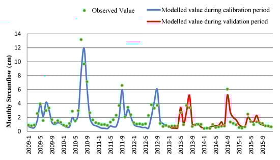
Figure 5.
Comparisons of monthly observed and modeling streamflows of Regional Nutrient Management (ReNuMa).
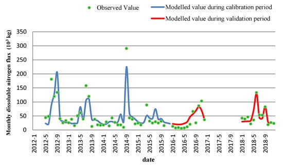
Figure 6.
Comparisons of monthly observed and modeling total dissolved nitrogen of Regional Nutrient Management (ReNuMa).
3.3. Changes of Streamflow
The estimates of the annual streamflow under various SSP scenarios in different future periods are illustrated in Figure 7. There were generally decreasing trends in the annual streamflow yields for most scenarios except SSP 1-26. For the two emission-controlled scenarios of SSP 1-26 and SSP 2-45, the annual streamflow initially decreased around the 2030s and then increased with a peak around the 2070s. The annual streamflow increased 7.83% in the 2070s under the strictly controlled scenario of SSP 1-26. For the two uncontrolled scenarios of SSP3-7.0 and SSP5-8.5, there was a relative peak in annual streamflow around the 2050s and then a decrease to a minimum around the 2070s. The annual streamflow decreased 3.27% in the 2070s under the moderate uncontrolled scenario of SSP 3-70. It was expected that there would be 2–3% decreases in annual streamflow by the end of this century for most scenarios except SSP 1-26, which assumed a strict limitation of warming below 2 °C. These results indicate that the warming trends of climate changes would result in lower water flows in the river channel, which probably result from the severe evapotranspiration that offsets the additional precipitation. Positive climate policies in controlling greenhouse gas emissions to mitigate global warming trends are effective in stabilizing the changes of watershed annual streamflow and benefit local water resource security.
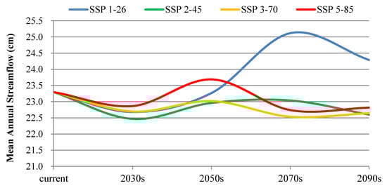
Figure 7.
Annual streamflow under various climate change scenarios in the future.
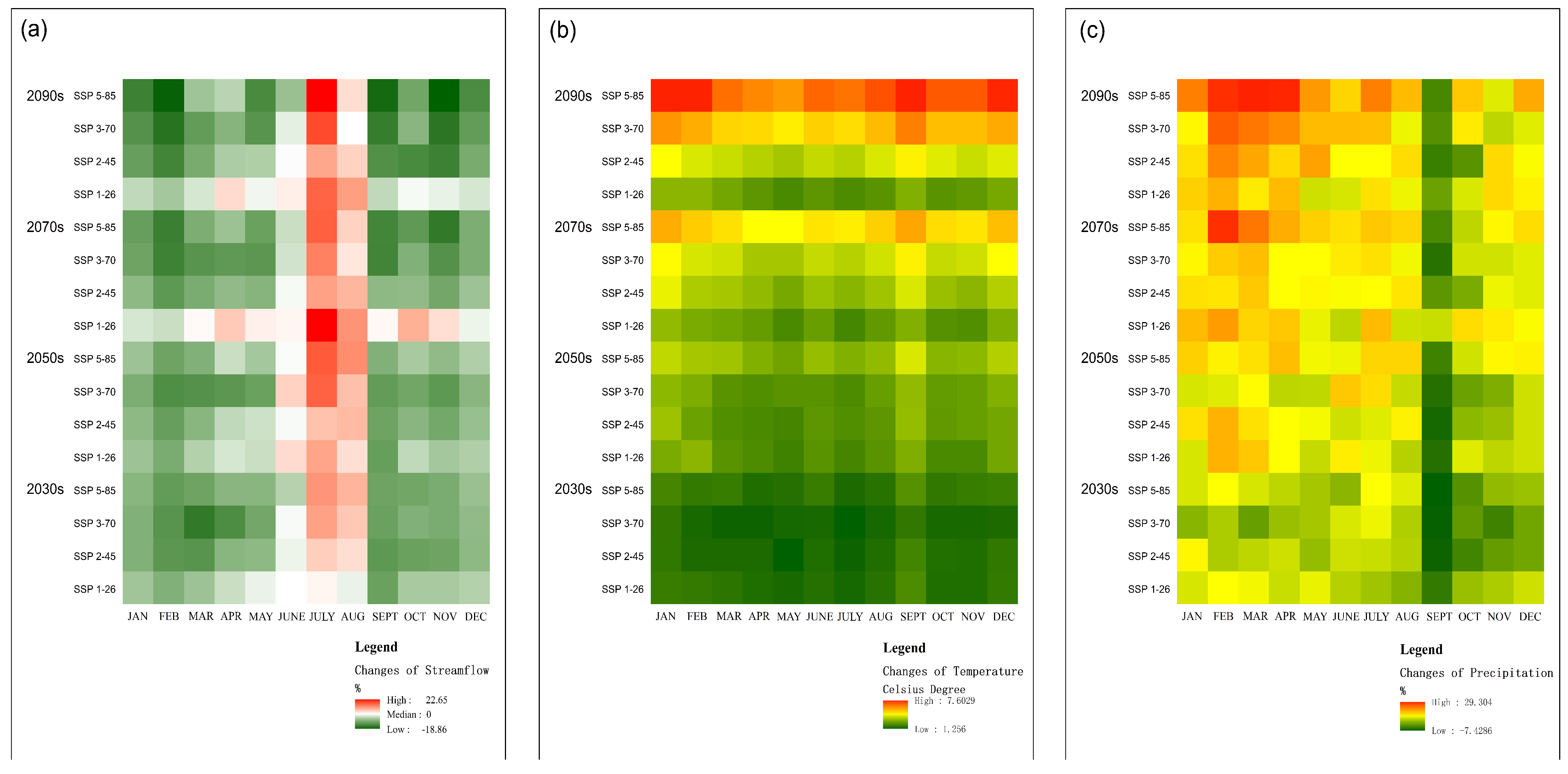
Another perspective on the changes in the monthly streamflows under various climate change scenarios in different future periods is shown in Figure 8, together with the changes in monthly temperatures and precipitation. General decreases in the streamflow were seen in most months, but remarkable increases of the monthly streamflow were observed during the summer for most scenarios in the future. The streamflow in July and August would increase for most SSP scenarios, and significant increases could be found in July. The expected monthly streamflow in July would increase 20.65% (10.11 mm) in the 2070s for the emission-controlled scenario of SSP 1-26 and 22.65% (11.08 mm) in the 2090s for the uncontrolled scenario of SSP 5-85, which integrated a great flood risk. In addition, there were significant decreases in the streamflow at the beginning and end of the winter in the future, especially for the uncontrolled scenarios. The expected monthly streamflow in December and February would decrease 18.86% (2.59 mm) and 18.64% (1.15 mm), respectively, in the 2090s under the SSP 5-85 scenario. In general, under the background of annual streamflow reduction, there would be significant changes in the time distribution characteristics of the water resources, with intensive humid trends in the summer months during the high-flow period but overall arid trends in other months, particularly during the low-flow period in winter. These changes should be of great concern for local water management to design effective projects for better water allocations to ensure the safety of residents’ lives from flood threats and to satisfy production needs, such as industrial consumption and agricultural irrigation.
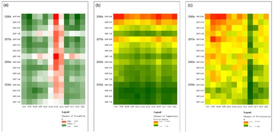
Figure 8.
Changes in monthly streamflow, temperature, and precipitation relative to current average monthly values under various climate change scenarios in the future. (a) The changing rates of the streamflow. (b) The amounts of change in temperature. (c) The changing rates of precipitation.
3.4. Changes of Dissolved Nitrogen Fluxes
The annual TDN fluxes in the future under different SSP scenarios are shown in Figure 9. It is evident that for all climate change scenarios in CMIP6, the annual TDN flux increased in the future. Continuous increases of the annual TDN flux were observed for the two uncontrolled scenarios of SSP3-7.0 and SSP5-8.5, which led to increases of 5.56% and 7.96% of the annual TDN flux in the study area around the 2090s. The changes in the annual TDN flux under the two emission-controlled scenarios of SSP 1-26 and SSP 2-45 gradually rose first and then fell, with peaks appearing around 2070s. The annual TDN flux in the 2070s increased 7.31% under the strictly controlled scenario of SSP 1-26 and 3.93% under the moderately controlled scenario of SSP 2-45. The annual TDN flux in the 2090s under SSP 1-26 and SSP 2-45 would decrease from the values around the 2070s, indicating positive effects of emission management on TDN flux control. The increased TDN fluxes mainly resulted from the additional non-point source pollution due to the increased transport of TDN associated with increases in the streamflow. More detailed measures concerning non-point pollution control are needed for local environmental management.
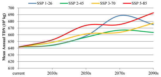
Figure 9.
Annual total dissolved nitrogen fluxes under various climate change scenarios in the future.
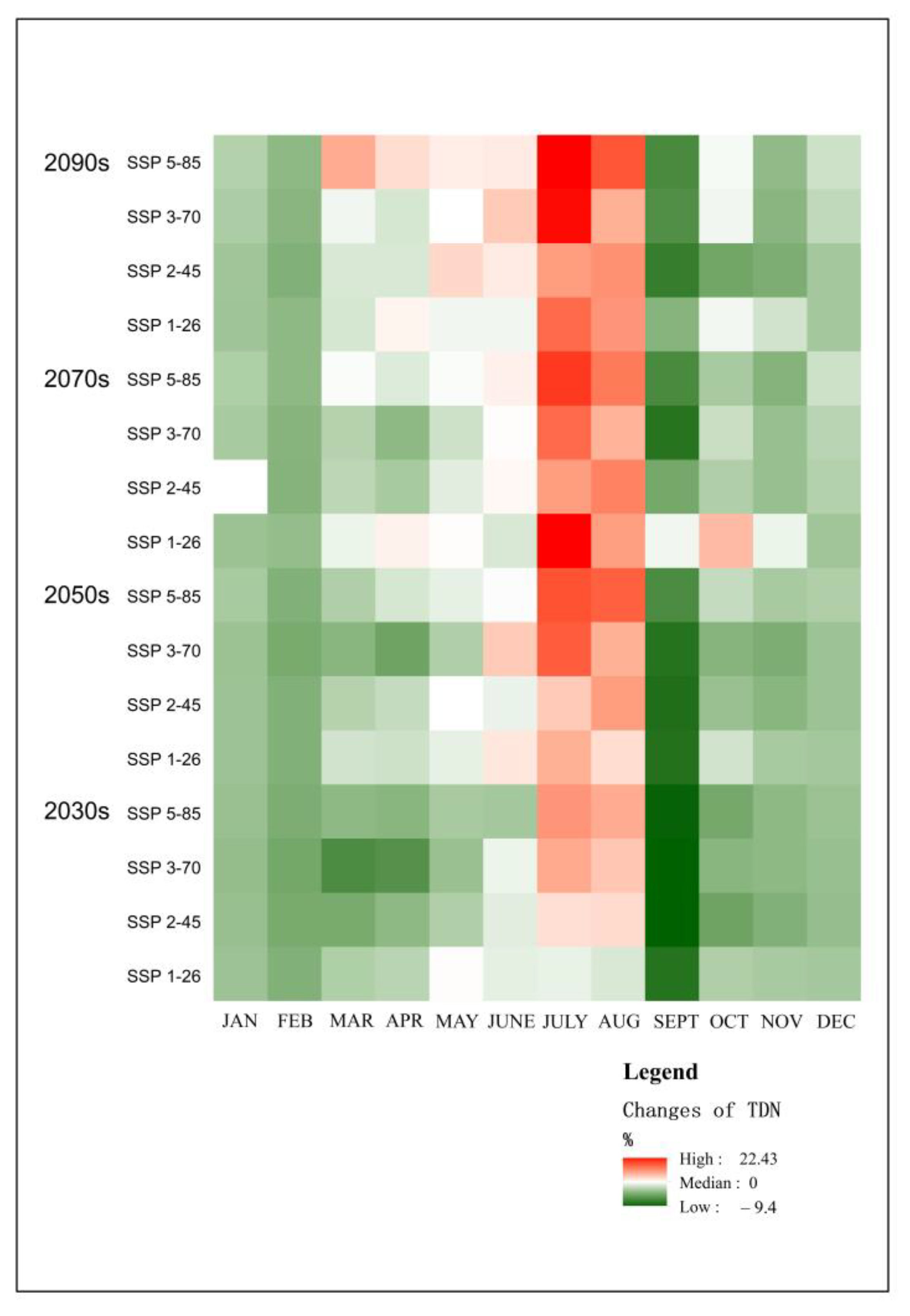
The changes in the monthly TDN fluxes in the future were similar to the changes in the monthly streamflow, which are illustrated in Figure 10. Against the increasing background of annual TDN fluxes, most changes in the monthly TDN fluxes were negative during the low-flow period in the winter. The increases in the monthly TDN fluxes in the summer were remarkable in the future. The peak of monthly TDN flux for the emission-controlled scenario of SSP 1-26 would occur in July around the 2070s, with an increase of 17.13% related to the current level. For the worst uncontrolled scenario of SSP 5-85, the peak of the monthly TDN fluxes during the research period could be found in July at the end of this century around the 2090s, with continuously increasing trends implying a worse situation in the next century. In general, the critical issues of TDN flux control in the summer were related to high summertime flows. The main pollution source under the changed climate status should be identified, and efficient measures should be projected to implement the best management practice, as discussed below in Section 3.5.

Figure 10.
Changes in monthly total dissolved nitrogen fluxes relative to current average monthly values under various climate change scenarios in the future.
3.5. Changes in Pollution Source Apportionments
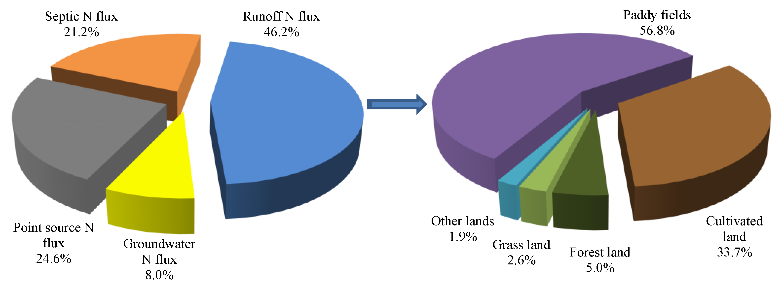
The current source apportionments of TDN in the study’s watershed estimated by ReNuMa are illustrated in Figure 11. There are generally four main routes for TDN loading: surface runoff, groundwater, septic system discharges, and point source discharges. The contributions of the point sources, which are discharged from the municipal sewage treatment plant of Yunxi town in the downstream area, comprised 24.6% of the total. The point source loads mainly include the domestic sewage of urban residents and industrial waste of the factories in Yunxi town. In addition, 21.2% TDN flux came from the septic systems of rural residents distributed in the upstream area. In addition, 8.0% of the TDN flux was contributed from groundwater, mainly resulting from the infiltration of polluted water and dissolutions of soil organic matter. Surface runoff contributed 46.2% of the TDN fluxes, mainly resulting from agricultural activities; 56.8% of the TDN in the runoff was from paddy fields, and 33.7% came from cultivated land, which mainly resulted from fertilizer and manure N in the runoff. A total of 9.5% of the TDN in the runoff came from forested land, grassland, water surfaces, and urban areas, which mainly resulted from atmospheric nitrogen deposition. Generally speaking, it is a mixed polluted watershed with significant non-point sources that may be sensitive to changes in the regional weather features.

Figure 11.
Source apportionments of total dissolved nitrogen in the study area.
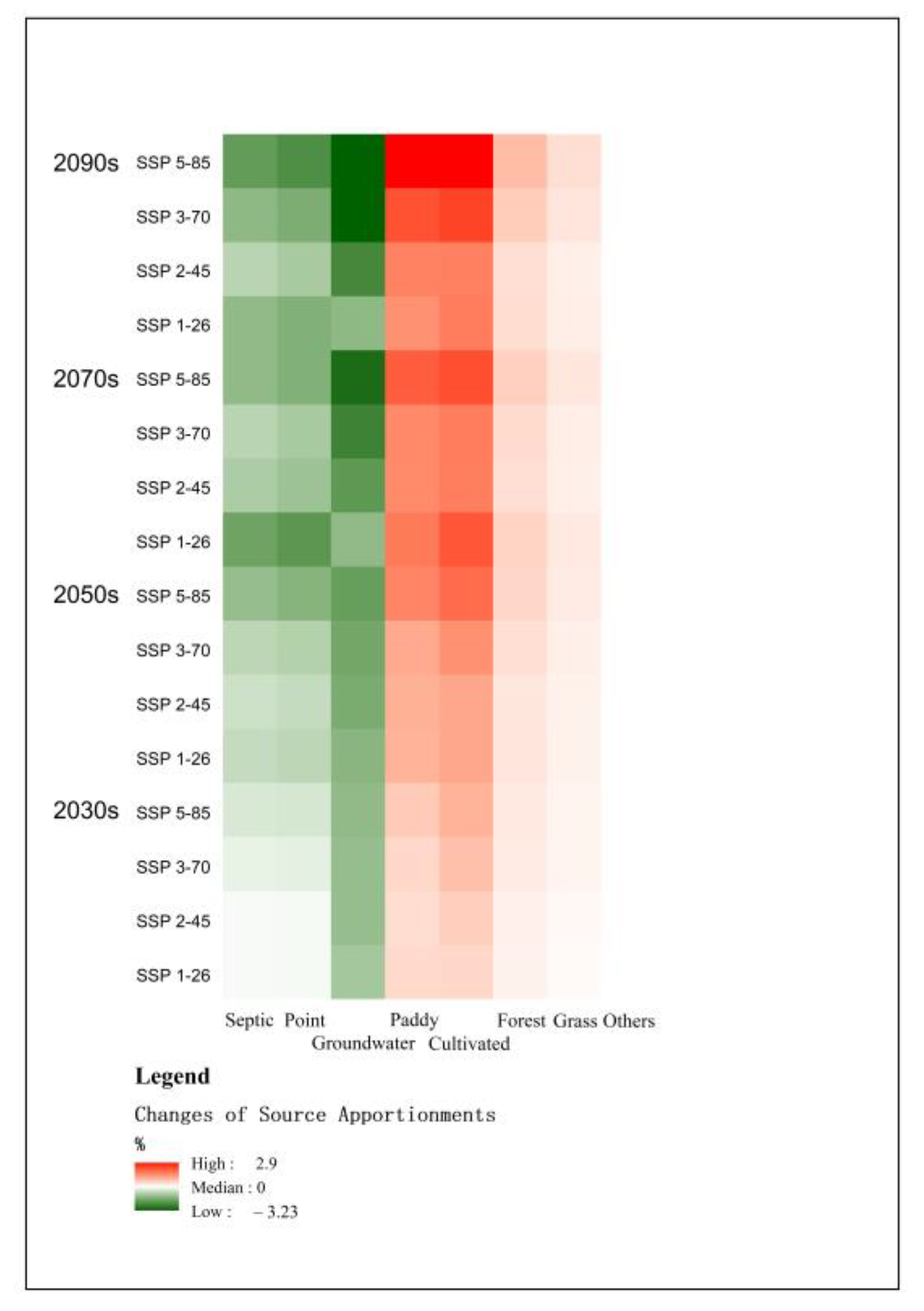
The changes in the source apportionments of TDN under various SSP scenarios in different future periods are shown in Figure 12. The proportions of the TDN loads contributed from natural land would increase, including those of paddy fields, cultivated land, forest land, and grassland. The relative contribution of TDN from the septic system (rural resident livings), point source, and groundwater would decrease. Because the absolute amounts of the point source contributions were assumed to be constant, decreases in their proportional contribution resulted from the increases in the total fluxes of TDN in the future. The impacts of climate changes on the TDN proportions due to groundwater and septic systems were negative. The absolute TDN yields from the septic system were generally steady, and the absolute TDN yields from groundwater were decreasing, which was more remarkable under the uncontrolled scenarios of SSP 3-70 and SSP 5-85 at the end of the 21st century. The changes in the contributing ratios of TDN from other land use areas in the future were negligible.

Figure 12.
The changes in pollution source apportionments of the total dissolved nitrogen fluxes relative to the current levels under various climate change scenarios in the future.
The critical changes in the source apportionments of the TDN under various climate change scenarios in the future focused on the natural land. There were generally increasing trends in the relative contributions of the TDN from the paddy fields, cultivated land, forest land, and grassland, implying significant increases in non-point source contributions in the future. The pollution contributed from the agricultural land use area of the paddy fields and cultivated lands were the main source of TDN loads in the study area in the future. The increases in relative contributions from agricultural land use area under the emission-controlled scenarios of SSP 1-26 and SSP 2-45 were smaller than those under the uncontrolled scenarios of SSP 3-70 and SSP 5-85. Both the absolute amounts and relative ratios would continue to grow under the two uncontrolled scenarios, with peaks at the end of the 21st century under the scenario of SSP 5-85. The changes in source contributions from the agricultural land use area were similar, with the changes in streamflow under the two emission-controlled scenarios, representing rising at first and then falling tends with peaks around the 2070s. It is obvious that the increasing TDN loads from the agricultural land use area mostly resulted from the more non-point source contributions due to the increases in streamflow in the future. These indicate that more non-point source control practices should be implemented by local watershed management in the future. To sum up, positive climate policies to address greenhouse gas emission controls are important to mitigate increases in TDN fluxes in the future, and more strict management of agricultural land for non-point source control will likely be needed, particularly during the high-flow periods in the summer, to avoid extreme events. It is necessary to project flexible strategies facing the changing climate status in the future to realize a dynamic best management practice including integrated measures [62,63], such as limits on crop fertilization, matching of the timing of fertilizer-to-crop demand, conservation tillage, terraces, and diversions to reduce soil and organic N loss, plant buffer structures, constructed wetlands, and so on.
3.6. Limitations
The first limitation of this combined modeling approach is the potential uncertainty in synthetic weather series generation. The local weather model is based on more than 60 years of historical data. These data are not nearly long enough, and potentially extreme weather conditions may be ignored. In addition, the LARS-WG model assumes that the site-scale climate feature is stable. However, in fact, climate change has been and is occurring, which will introduce some uncertainty in the parameter estimations of the weather generator.
The second limitation is the limited GCM outputs. As an ongoing project, the global GCMs experiment based on CMIP6 has not yet been completed. Many GCM outputs are not complete yet, with limited scenarios or periods which are difficult to use for the ensemble. In addition, the estimations of these GCM outputs are still in progress, and some outputs may have potential uncertainties in some areas.
The third limitation is the relatively long time step of ReNuMa, which led us to only get monthly streamflow and TDN results at most. We can estimate that there will be extreme situations in a certain month. However, it is difficult to judge whether these changes occur concentrated in a few days and what the state of the extreme day is, which is more important for risk management.
The existing assessment results provided in this article can provide us a perspective on the impacts of future climate change on the watershed. It can help us to understand the changes of future streamflow and the TDN in different situations and periods and to prove the rationality of proactive environmental policies. Future research is expected to focus on more refined simulations and detailed management suggestions. More detailed watershed scale downscaling with selected GCM outputs based on a complete dataset of CMIP 6 GCM experiments would greatly reduce the uncertainty caused by the data factors. More detailed modeling for the watershed hydrochemical processes would provide short-term extreme status estimations and more accurately reflect the effects of management measures and carry out scenario analysis for Best Management Practices (BMPs).
4. Conclusions
The changes in the watershed streamflow and TDN in the Tianhe River in China were estimated based on CMIP6-SSP scenarios. Four main conclusions can be drawn from the results of the present study:
- Based on the agreement between the observations and modeling results, the proposed approach of the combined application of the LARS-WG and ReNuMa model appears to be a valid approach to estimate climate change impacts on a watershed hydrochemical process using CMIP6-SSP scenarios. It can be used as an alternative approach in other similar areas for climate change impact estimations.
- There were generally decreasing trends for the annual streamflow responding to the climate changes in the future. However, monthly distributions of the annual streamflow will change from the historical patterns in the study area, with large increases in streamflow occurring in the summer months, resulting in flood risk. Generally, decreases in streamflow occurred during the low-flow periods, resulting in drought risk. Climate policies to control greenhouse gas emissions will be needed to mitigate the impacts of climate changes on the watershed’s hydrological characteristics.
- Increasing trends in annual TDN fluxes occurred in response to the climate changes in the future. The increases in monthly TDN fluxes mainly focused on the summer during the high-flow periods due to the additional non-point source contributions from agricultural lands. Policies to control the impact of human activities on climate changes would also mitigate predicted changes in the TDN fluxes, and more strict measures concerning non-point source control should be implemented in the summer for local water management in the future.
- The main limitation of this study is the uncertainty caused by the limited data and modeling tools. The GCM experiments based on CMIP 6 are ongoing, with limited outputs published. Site-scale weather downscaling is limited in presenting watershed spatial variation. The monthly watershed hydrological modeling is limited in providing detailed short-term extreme information. Future research is expected to provide more detailed estimations and focus on more practical uses in management for the BMPs.
Supplementary Materials
The following are available online at https://www.mdpi.com/article/10.3390/su131810102/s1.
Author Contributions
Conceptualization, J.S. and J.Y.; methodology, J.S.; software, X.L.; validation, J.Y. and X.L.; formal analysis, J.S.; investigation, J.S. and X.L.; resources, J.Y.; data curation, J.S.; writing—original draft preparation, J.S.; writing—review and editing, J.Y.; visualization, X.L.; supervision, J.Y.; project administration, J.Y.; funding acquisition, J.Y. All authors have read and agreed to the published version of the manuscript.
Funding
This research was funded by the Science & Technology Development Fund of Tianjin Education Commission for Higher Education, grant number 2018KJ160.
Institutional Review Board Statement
Not applicable.
Informed Consent Statement
Not applicable.
Data Availability Statement
Not applicable.
Acknowledgments
The authors would like to acknowledge Dennis P. Swaney from Cornell University for his contributions to the manuscript, with valuable scientific comments and high-quality language editing. We also acknowledge the World Climate Research Programme which, through its Working Group on Coupled Modeling, coordinated and promoted CMIP6. We thank the climate modeling groups for producing and making available their model output, the Earth System Grid Federation (ESGF) for archiving the data and providing access, and the multiple funding agencies who support CMIP6 and ESGF. In addition, the authors would like to acknowledge the WorldClim data website (http://www.worldclim.org, 1 July 2021) for the high spatial resolution global weather and climate data. Aside from that, we acknowledge the China Meteorological Data Service Centre (http://data.cma.cn, 1 July 2021) for the long-term historic weather data of the study area.
Conflicts of Interest
The authors declare no conflict of interest.
Abbreviations
| SSP | Shared Socioeconomic Pathways |
| CMIP6 | Coupled Model Intercomparison Project Phase 6 |
| TDN | Total Dissolved Nitrogen |
| GCMs | General Circulation Models |
| LARS-WG | Long Ashton Research Station Weather Generator |
| ReNuMa | Regional Nutrient Management |
| NANI | Net Anthropogenic Nitrogen Inputs |
| WGCM | Working Group on Coupled Modeling |
| DOE | US Department of Energy |
| PCMDI | Program for Climate Model Diagnosis and Intercomparison |
| IPCC | Intergovernmental Panel on Climate Change |
| RCM | Regional Climate Models |
| CNN | Convolutional Neural Network |
References
- Woolway, R.I.; Jennings, E.; Shatwell, T.; Golub, M.; Pierson, D.C.; Maberly, S.C. Lake heatwaves under climate change. Nature 2021, 589, 402–407. [Google Scholar] [CrossRef] [PubMed]
- Descombes, P.; Pitteloud, C.; Glauser, G.; Defossez, E.; Kergunteuil, A.; Allard, P.-M.; Rasmann, S.; Pellissier, L. Novel trophic interactions under climate change promote alpine plant coexistence. Science 2020, 370, 1469–1473. [Google Scholar] [CrossRef]
- Halsch, C.A.; Shapiro, A.M.; Fordyce, J.A.; Nice, C.C.; Thorne, J.H.; Waetjen, D.P.; Forister, M.L. Insects and recent climate change. Proc. Natl. Acad. Sci. USA 2021, 118, e2002543117. [Google Scholar] [CrossRef]
- Liu, Y.; Chen, J. Future global socioeconomic risk to droughts based on estimates of hazard, exposure, and vulnerability in a changing climate. Sci. Total Environ. 2021, 751, 142159. [Google Scholar] [CrossRef]
- Chen, S.; Gong, B. Response and adaptation of agriculture to climate change: Evidence from China. J. Dev. Econ. 2021, 148, 102557. [Google Scholar] [CrossRef]
- Yuan, S.; Quiring, S.M.; Kalcic, M.M.; Apostel, A.M.; Evenson, G.R.; Kujawa, H.A. Optimizing climate model selection for hydrological modeling: A case study in the Maumee River basin using the SWAT. J. Hydrol. 2020, 588, 125064. [Google Scholar] [CrossRef]
- Kujawa, H.; Kalcic, M.; Martin, J.; Aloysius, N.; Apostel, A.; Kast, J.; Murumkar, A.; Evenson, G.; Becker, R.; Boles, C.; et al. The hydrologic model as a source of nutrient loading uncertainty in a future climate. Sci. Total Environ. 2020, 724, 138004. [Google Scholar] [CrossRef] [PubMed]
- Szalińska, E.; Zemełka, G.; Kryłów, M.; Orlińska-Woźniak, P.; Jakusik, E.; Wilk, P. Climate change impacts on contaminant loads delivered with sediment yields from different land use types in a Carpathian basin. Sci. Total Environ. 2021, 755, 142898. [Google Scholar] [CrossRef] [PubMed]
- Zaninelli, P.G.; Menéndez, C.G.; Falco, M.; López-Franca, N.; Carril, A.F. Future hydroclimatological changes in South America based on an ensemble of regional climate models. Clim. Dyn. 2019, 52, 819–830. [Google Scholar] [CrossRef]
- Konapala, G.; Mishra, A.K.; Wada, Y.; Mann, M.E. Climate change will affect global water availability through compounding changes in seasonal precipitation and evaporation. Nat. Commun. 2020, 11, 3044. [Google Scholar] [CrossRef] [PubMed]
- Akbas, A.; Freer, J.; Ozdemir, H.; Bates, P.D.; Turp, M.T. What about reservoirs? Questioning anthropogenic and climatic interferences on water availability. Hydrol. Process. 2020, 34, 5441–5455. [Google Scholar] [CrossRef]
- Liu, Z.; Herman, J.D.; Huang, G.; Kadir, T.; Dahlke, H.E. Identifying climate change impacts on surface water supply in the southern Central Valley, California. Sci. Total Environ. 2021, 759, 143429. [Google Scholar] [CrossRef]
- Shrestha, A.; Shrestha, S.; Tingsanchali, T.; Budhathoki, A.; Ninsawat, S. Adapting hydropower production to climate change: A case study of Kulekhani Hydropower Project in Nepal. J. Clean. Prod. 2021, 279, 123483. [Google Scholar] [CrossRef]
- Ercan, M.B.; Maghami, I.; Bowes, B.D.; Morsy, M.M.; Goodall, J.L. Estimating Potential Climate Change Effects on the Upper Neuse Watershed Water Balance Using the SWAT Model. JAWRA J. Am. Water Resour. Assoc. 2020, 56, 53–67. [Google Scholar] [CrossRef]
- Giri, S.; Lathrop, R.G.; Obropta, C.C. Climate change vulnerability assessment and adaptation strategies through best management practices. J. Hydrol. 2020, 580, 124311. [Google Scholar] [CrossRef]
- Gorelick, D.E.; Lin, L.; Zeff, H.B.; Kim, Y.; Vose, J.M.; Coulston, J.W.; Wear, D.N.; Band, L.E.; Reed, P.M.; Characklis, G.W. Accounting for Adaptive Water Supply Management When Quantifying Climate and Land Cover Change Vulnerability. Water Resour. Res. 2020, 56, e2019WR025614. [Google Scholar] [CrossRef]
- Xu, X.; Wang, Y.-C.; Kalcic, M.; Muenich, R.L.; Yang, Y.C.E.; Scavia, D. Evaluating the impact of climate change on fluvial flood risk in a mixed-use watershed. Environ. Modell. Softw. 2019, 122, 104031. [Google Scholar] [CrossRef]
- Sha, J.; Wang, Z.-L.; Lu, R.; Zhao, Y.; Li, X.; Shang, Y.-T. Estimation of the Source Apportionment of Phosphorus and Its Responses to Future Climate Changes Using Multi-Model Applications. Water 2018, 10, 468. [Google Scholar] [CrossRef] [Green Version]
- Ndhlovu, G.Z.; Woyessa, Y.E. Modeling impact of climate change on catchment water balance, Kabompo River in Zambezi River Basin. J. Hydrol. Reg. Stud. 2020, 27, 100650. [Google Scholar] [CrossRef]
- Xu, H.; Liu, L.; Wang, Y.; Wang, S.; Hao, Y.; Ma, J.; Jiang, T. Assessment of climate change impact and difference on the river runoff in four basins in China under 1.5 and 2.0 °C global warming. Hydrol. Earth Syst. Sci. 2019, 23, 4219–4231. [Google Scholar] [CrossRef] [Green Version]
- Eyring, V.; Bony, S.; Meehl, G.A.; Senior, C.A.; Stevens, B.; Stouffer, R.J.; Taylor, K.E. Overview of the Coupled Model Intercomparison Project Phase 6 (CMIP6) experimental design and organization. Geosci. Model Dev. 2016, 9, 1937–1958. [Google Scholar] [CrossRef] [Green Version]
- Gidden, M.J.; Riahi, K.; Smith, S.J.; Fujimori, S.; Luderer, G.; Kriegler, E.; van Vuuren, D.P.; van den Berg, M.; Feng, L.; Klein, D.; et al. Global emissions pathways under different socioeconomic scenarios for use in CMIP6: A dataset of harmonized emissions trajectories through the end of the century. Geosci. Model Dev. 2019, 12, 1443–1475. [Google Scholar] [CrossRef] [Green Version]
- Petrie, R.; Denvil, S.; Ames, S.; Levavasseur, G.; Fiore, S.; Allen, C.; Antonio, F.; Berger, K.; Bretonnière, P.A.; Cinquini, L.; et al. Coordinating an operational data distribution network for CMIP6 data. Geosci. Model Dev. 2021, 14, 629–644. [Google Scholar] [CrossRef]
- Huang, S.; Wang, F.; Elliott, E.M.; Zhu, F.; Zhu, W.; Koba, K.; Yu, Z.; Hobbie, E.A.; Michalski, G.; Kang, R.; et al. Multiyear Measurements on Delta17O of Stream Nitrate Indicate High Nitrate Production in a Temperate Forest. Environ. Sci. Technol. 2020, 54, 4231–4239. [Google Scholar] [CrossRef]
- Ge, F.; Zhu, S.; Luo, H.; Zhi, X.; Wang, H. Future changes in precipitation extremes over Southeast Asia: Insights from CMIP6 multi-model ensemble. Environ. Res. Lett. 2021, 16, 024013. [Google Scholar] [CrossRef]
- Kreienkamp, F.; Lorenz, P.; Geiger, T. Statistically Downscaled CMIP6 Projections Show Stronger Warming for Germany. Atmosphere 2020, 11, 1245. [Google Scholar] [CrossRef]
- Lin, X.; Huang, G.; Piwowar, J.M.; Zhou, X.; Zhai, Y. Risk of hydrological failure under the compound effects of instant flow and precipitation peaks under climate change: A case study of Mountain Island Dam, North Carolina. J. Clean. Prod. 2021, 284, 125305. [Google Scholar] [CrossRef]
- Sanyal, J.; Wesley Lauer, J.; Kanae, S. Examining the downstream geomorphic impact of a large dam under climate change. CATENA 2021, 196, 104850. [Google Scholar] [CrossRef]
- Tan, M.L.; Gassman, P.W.; Yang, X.; Haywood, J. A review of SWAT applications, performance and future needs for simulation of hydro-climatic extremes. Adv. Water Resour. 2020, 143, 103662. [Google Scholar] [CrossRef]
- Di Sante, F.; Coppola, E.; Giorgi, F. Projections of river floods in Europe using EURO-CORDEX, CMIP5 and CMIP6 simulations. Int. J. Climatol. N/A 2021, 41, 3203–3221. [Google Scholar] [CrossRef]
- Martinez-Villalobos, C.; Neelin, J.D. Climate models capture key features of extreme precipitation probabilities across regions. Environ. Res. Lett. 2021, 16, 024017. [Google Scholar] [CrossRef]
- Miralha, L.; Muenich, R.L.; Scavia, D.; Wells, K.; Steiner, A.L.; Kalcic, M.; Apostel, A.; Basile, S.; Kirchhoff, C.J. Bias correction of climate model outputs influences watershed model nutrient load predictions. Sci. Total Environ. 2021, 759, 143039. [Google Scholar] [CrossRef] [PubMed]
- Zhang, D.; Tan, M.L.; Dawood, S.R.S.; Samat, N.; Chang, C.K.; Roy, R.; Tew, Y.L.; Mahamud, M.A. Comparison of NCEP-CFSR and CMADS for Hydrological Modeling Using SWAT in the Muda River Basin, Malaysia. Water 2020, 12, 3288. [Google Scholar] [CrossRef]
- Guo, Y.; Fang, G.; Xu, Y.-P.; Tian, X.; Xie, J. Responses of hydropower generation and sustainability to changes in reservoir policy, climate and land use under uncertainty: A case study of Xinanjiang Reservoir in China. J. Clean. Prod. 2021, 281, 124609. [Google Scholar] [CrossRef]
- Jose, D.M.; Dwarakish, G.S. Uncertainties in predicting impacts of climate change on hydrology in basin scale: A review. Arab. J. Geosci. 2020, 13, 1037. [Google Scholar] [CrossRef]
- Xu, Z.; Han, Y.; Yang, Z. Dynamical downscaling of regional climate: A review of methods and limitations. Sci. China Earth Sci. 2019, 62, 365–375. [Google Scholar] [CrossRef]
- Dai, A.; Rasmussen, R.M.; Ikeda, K.; Liu, C. A new approach to construct representative future forcing data for dynamic downscaling. Clim. Dyn. 2020, 55, 315–323. [Google Scholar] [CrossRef]
- Li, X.; Babovic, V. Multi-site multivariate downscaling of global climate model outputs: An integrated framework combining quantile mapping, stochastic weather generator and Empirical Copula approaches. Clim. Dyn. 2019, 52, 5775–5799. [Google Scholar] [CrossRef]
- Baño-Medina, J.; Manzanas, R.; Gutiérrez, J.M. Configuration and intercomparison of deep learning neural models for statistical downscaling. Geosci. Model Dev. 2020, 13, 2109–2124. [Google Scholar] [CrossRef]
- Stengel, K.; Glaws, A.; Hettinger, D.; King, R.N. Adversarial super-resolution of climatological wind and solar data. Proc. Natl. Acad. Sci. USA 2020, 117, 16805–16815. [Google Scholar] [CrossRef]
- Gebrechorkos, S.H.; Bernhofer, C.; Hülsmann, S. Climate change impact assessment on the hydrology of a large river basin in Ethiopia using a local-scale climate modeling approach. Sci. Total Environ. 2020, 742, 140504. [Google Scholar] [CrossRef] [PubMed]
- Martin, N. Watershed-Scale, Probabilistic Risk Assessment of Water Resources Impacts from Climate Change. Water 2021, 13, 40. [Google Scholar] [CrossRef]
- Mukundan, R.; Acharya, N.; Gelda, R.K.; Frei, A.; Owens, E.M. Modeling streamflow sensitivity to climate change in New York City water supply streams using a stochastic weather generator. J. Hydrol. Reg. Stud. 2019, 21, 147–158. [Google Scholar] [CrossRef]
- Fick, S.E.; Hijmans, R.J. WorldClim 2: New 1-km spatial resolution climate surfaces for global land areas. Int. J. Climatol. 2017, 37, 4302–4315. [Google Scholar] [CrossRef]
- Haith, D.A.; Shoemaker, L.L. GENERALIZED WATERSHED LOADING FUNCTIONS FOR STREAM FLOW NUTRIENTS1. JAWRA J. Am. Water Resour. Assoc. 1987, 23, 471–478. [Google Scholar] [CrossRef]
- Hong, B.; Swaney, D.P.; Howarth, R.W. A toolbox for calculating net anthropogenic nitrogen inputs (NANI). Environ. Model. Softw. 2011, 26, 623–633. [Google Scholar] [CrossRef]
- Hu, M.; Liu, Y.; Wang, J.; Dahlgren, R.A.; Chen, D. A modification of the Regional Nutrient Management model (ReNuMa) to identify long-term changes in riverine nitrogen sources. J. Hydrol. 2018, 561, 31–42. [Google Scholar] [CrossRef] [Green Version]
- Sha, J.; Liu, M.; Wang, D.; Swaney, D.P.; Wang, Y. Application of the ReNuMa model in the Sha He river watershed: Tools for watershed environmental management. J. Environ. Manag. 2013, 124, 40–50. [Google Scholar] [CrossRef]
- Li, Z.; Liu, M.; Zhao, Y.; Liang, T.; Sha, J.; Wang, Y. Application of Regional Nutrient Management Model in Tunxi Catchment: In Support of the Trans-boundary Eco-compensation in Eastern China. CLEAN Soil Air Water 2014, 42, 1729–1739. [Google Scholar] [CrossRef]
- Sha, J.; Zhao, Y.; Li, X.; Wang, Z.-l. Assessing impacts of future climate change on hydrological processes in an urbanizing watershed with a multimodel approach. J. Water Clim. Chang. 2020, 12, 1023–1042. [Google Scholar] [CrossRef]
- Solvers, F. Standard excel solver—limitations of nonlinear optimization. 2019. Available online: https://www.solver.com/standard-excel-solver-limitations-nonlinear-optimization (accessed on 1 July 2021).
- Sha, J.; Swaney, D.P.; Hong, B.; Wang, J.; Wang, Y.; Wang, Z.-L. Estimation of watershed hydrologic processes in arid conditions with a modified watershed model. J. Hydrol. 2014, 519, 3550–3556. [Google Scholar] [CrossRef]
- Semenov, M.A.; Stratonovitch, P. Adapting wheat ideotypes for climate change: Accounting for uncertainties in CMIP5 climate projections. Clim. Res. 2015, 65, 123–139. [Google Scholar] [CrossRef] [Green Version]
- Ma, D.; Qian, B.; Gu, H.; Sun, Z.; Xu, Y.-P. Assessing climate change impacts on streamflow and sediment load in the upstream of the Mekong River basin. Int. J. Climatol. N/A 2021, 41, 3391–3410. [Google Scholar] [CrossRef]
- Morid, R.; Shimatani, Y.; Sato, T. An integrated framework for prediction of climate change impact on habitat suitability of a river in terms of water temperature, hydrological and hydraulic parameters. J. Hydrol. 2020, 587, 124936. [Google Scholar] [CrossRef]
- Sha, J.; Li, X.; Wang, Z.-L. Estimation of future climate change in cold weather areas with the LARS-WG model under CMIP5 scenarios. Theor. Appl. Climatol. 2019, 137, 3027–3039. [Google Scholar] [CrossRef]
- Kavwenje, S.; Zhao, L.; Chen, L.; Chaima, E. Projected temperature and precipitation changes using the LARS-WG statistical downscaling model in the Shire River Basin, Malawi. Int. J. Climatol. N/A 2021. [Google Scholar] [CrossRef]
- Bayatvarkeshi, M.; Zhang, B.; Fasihi, R.; Adnan, R.M.; Kisi, O.; Yuan, X. Investigation into the Effects of Climate Change on Reference Evapotranspiration Using the HadCM3 and LARS-WG. Water 2020, 12, 666. [Google Scholar] [CrossRef] [Green Version]
- Li, X.; Sha, J.; Zhao, Y.; Wang, Z.-L. Estimating the Responses of Hydrological and Sedimental Processes to Future Climate Change in Watersheds with Different Landscapes in the Yellow River Basin, China. Int. J. Environ. Res. Public Health 2019, 16, 4054. [Google Scholar] [CrossRef] [PubMed] [Green Version]
- Khorshidi, M.S.; Nikoo, M.R.; Sadegh, M.; Nematollahi, B. A Multi-Objective Risk-Based Game Theoretic Approach to Reservoir Operation Policy in Potential Future Drought Condition. Water Resour. Manag. 2019, 33, 1999–2014. [Google Scholar] [CrossRef]
- Santos, F.M.d.; de Oliveira, R.P.; Mauad, F.F. Evaluating a parsimonious watershed model versus SWAT to estimate streamflow, soil loss and river contamination in two case studies in Tietê river basin, São Paulo, Brazil. J. Hydrol. Reg. Stud. 2020, 29, 100685. [Google Scholar] [CrossRef]
- Liu, G.; Chen, L.; Wei, G.; Shen, Z. New framework for optimizing best management practices at multiple scales. J. Hydrol. 2019, 578, 124133. [Google Scholar] [CrossRef]
- Saleem, S.; Levison, J.; Parker, B.; Martin, R.; Persaud, E. Impacts of Climate Change and Different Crop Rotation Scenarios on Groundwater Nitrate Concentrations in a Sandy Aquifer. Sustainability 2020, 12, 1153. [Google Scholar] [CrossRef] [Green Version]


Publisher’s Note: MDPI stays neutral with regard to jurisdictional claims in published maps and institutional affiliations. |
© 2021 by the authors. Licensee MDPI, Basel, Switzerland. This article is an open access article distributed under the terms and conditions of the Creative Commons Attribution (CC BY) license (https://creativecommons.org/licenses/by/4.0/).