Student-Performulator: Student Academic Performance Using Hybrid Deep Neural Network

Abstract

Educational data generated through various platforms such as e-learning, e-admission systems, and automated result management systems can be effectively processed through educational data mining techniques in order to gather highly useful insights into students’ performance. The prediction of student performance from historical academic data is a highly desirable application of educational data mining. In this regard, there is an urgent need to develop an automated technique for student performance prediction. Existing studies on student performance prediction primarily focus on utilizing the conventional feature representation schemes, where extracted features are fed to a classifier. In recent years, deep learning has enabled researchers to automatically extract high-level features from raw data. Such advanced feature representation schemes enable superior performance in challenging tasks. In this work, we examine the deep neural network model, namely, the attention-based Bidirectional Long Short-Term Memory (BiLSTM) network to efficiently predict student performance (grades) from historical data. In this article, we have used the most advanced BiLSTM combined with an attention mechanism model by analyzing existing research problems, which are based on advanced feature classification and prediction. This work is really vital for academicians, universities, and government departments to early predict the performance. The superior sequence learning capabilities of BiLSTM combined with attention mechanism yield superior performance compared to the existing state-of-the-art. The proposed method has achieved a prediction accuracy of 90.16%.

1. Introduction

In the Sustainable Development Goals, quality education plays an important role which is approved by the United Nations [1], this is also an important and basic challenge for supporting sustainable development globally.

The gradual increase in education data is due to the continuous generation of such data from different sources, such as e-learning, learning management systems, admission systems, and student feedback analysis systems. The student data acquired from the aforementioned sources are used for making a simple query-level decision, whereas a huge bulk of data remains unused due to the complex and noisy nature of datasets. Student-related educational data have received considerable attention from researchers in the field of Educational Data Mining (EDP) for finding useful information, such as the prediction of student performance [2]. Therefore, it is an essential task to investigate and apply state-of-the-art deep learning techniques in the domain of Educational Data Mining (EDM) for efficient prediction of performance from students’ historical data.

The assessment of student performance from historical data has been investigated by different researchers by employing EDM techniques. The main emphasis of these works is on the early prediction of student performance in terms of marks, grades, and pass/fail. However, prediction of student academic performance from noisy and large datasets is a challenging task due to the following major limitations associated with the existing works: (i) poor selection of predictor variables describing the student performance, and (ii) use of machine learning techniques, based on feature classical representation schemes followed by a classifier.

The authors studied the machine learning-based technique for the prediction of student performance using historical data. In the baseline study, different ML classifiers are used to predict student performance in terms of binary classes (pass/fail). However, prediction of performance in terms of pass/fail does not provide a deeper insight into student’s academic assessment. Another major drawback of their technique is that it is deficient in terms of evaluating the overall dependencies pertaining to predictor variables in the student data. Therefore, the classical machine learning classifiers do not provide an efficient mechanism for predicting student performance from academic data.

To overcome the drawbacks associated with the baseline study, we employ an improved feature selection technique followed by a deep neural network model, which has successfully been used in different applications such as rumor detection, extremist affiliation detection, and other domains. We propose to employ a Chi-Square test for feature selection and the attention-based BiLSTM model for student grade prediction. It works as follows: (i) in the feature selection module, the Chi-Square test extracts the most appropriate high ranked features having a significant role in student grade prediction, and (ii) the Bidirectional Long Short-Term Memory (BiLSTM) considers the contextual information of the past as well as the future, and (iii) the attention mechanism has also been introduced to capture the most significant features from the given student data. Therefore, the proposed technique takes advantage of the functionalities of both improved feature selection and BiLSTM, along with the attention layer, to predict students’ final grades on the basis of their historical academic performance.

The prediction of grades (performance) from students’ historical academic data faces different challenges, such as poor selection of predictor variables, the small size of the dataset labeled with binary classes (pass/fail). Additionally, the machine learning technique is applied to predict student grades. To overcome these issues, we take the task of student grade prediction from historical data as the multi-label classification problem, in which, from the given input student data, final grade G3 is predicted as “A1”, “A”, “B”, “C”, “D”, “E”, or “F”. A sequence of student’s performance training data D $=\left[td1,td2,\dots ..tdn\right]$ is taken as input by the deep learning method to predict the final grade G3$ϵ \left[0\dots .6\right]$, i.e., 0 if A1, 1 for A, etc., and 6 for F. Our goal is to build an automatic technique that learns from the given data and labels, to accurately predict the respective class labels (student grade). The aim of the study is to build a computation model based on improved feature selection and hybrid deep neural network in the domain of EDM, which is trained over student academic performance historical data, and which can predict student final grade.

Our aim at the development of a deep neural network model is based on improved feature selection. Firstly, a statistical technique, namely the Chi-Square test, is applied to select the most appropriate predictor variables for student grade prediction. In the next step, the Bidirectional Long Short-Term Memory (BiLSTM) is applied, where the forward LSTM keeps track of future information and backward LSTM manipulates past information. Finally, the attention layer is introduced to implement an attention mechanism to capture the most significant features from the given student data.

The presented work is organized as follows. In Section 2 the related research work is discussed, in Section 3, the methodologies and experimental evaluation are discussed. Similarly, in Section 4, detailed experimental works are carried in the shape of results and discussion. In the last section, a discussion and conclusion of our proposed system is discussed.

2. Related Work

A lot of research work in the past was carried in the field of the topic of educational data mining, and it is still a hot research area in machine and deep learning. Different methodologies and tools are used to visualize and analyze the data, and the main aim of many researchers is to develop an automatic system that can predict the grades, marks, institution rating, and institution recommendation. In this section, some state-of-the-art research works are discussed, which can assist in identifying the research gap and propose the methodology.

While working on student performance prediction, the authors proposed an ML technique by predicting student grades in terms of pass/fail. However, the system’s performance can be further improved by using automatic feature representation schemes used in DL models and further extending the predicted classes to multi-level, i.e., assignment of grades into multiple classes, such as “outstanding”, “excellent”, and others.

The study conducted by [3] described the application of big data in the field of education. The big data techniques are incorporated in different ways for learning analytics i.e., performance prediction of a system, data visualization, risk detection, student skills estimation, course recommendation system, fraud detection, student grouping, and collaboration among other students. The functionality of the predictive analysis is emphasized in this study with a special focus on student performance, behavior, and skills prediction.

The study conducted by [4] aims at developing a collaborative filtering technique to predict the students’ performance using academic records. The experimental results show that the method is effective as compared to the baseline support vector machine classifier. In their work on student performance evaluation, [5] proposed a technique based on low-range matrix factorization and dispersed linear model, which takes students’ historical academic grade data as an input with the aim to estimate the performance of a student. The dataset is comprised of student academic instances of about 12.5 years collected from the University of Minnesota. The proposed system shows improvement in grade prediction accuracy.

In [6], a novel approach is proposed by extracting education data using a recommendation system. The system is specially designed to predict student performance using an educational context such as matrix factorization. The recommendation system is validated by comparing it with other state-of-the-art regression models such as linear and logistic regression. Another contribution of the proposed system is an application of the recommendation system.

In their work on building a student classification system, [7] proposed a machine learning-based technique by using two state-of-the-art classifiers i.e., decision tree and Naïve Bayes. The dataset was collected from various secondary schools. It was observed that among other features, “father occupation” played an important role to improve the accuracy of the final grade prediction system. The experimental results show that the decision tree classifier performed better in terms of accuracy than the Naïve Bayes classifier.

The authors in [8] focused on tools, techniques, and big data algorithms used in the education context to facilitate and provide benefit in the learning and teaching process. The authors have reported a relationship between the education environment and big data. A smart recommendation system, based on using Spark and Hadoop, is proposed by [9] to find the relationship between the student academic activities. For this purpose, unsupervised machine learning technique, namely association rule mining. The rules are extracted using a rule mining algorithm and the student behavior is used to catalog the courses. The obtained results show the effectiveness of the proposed recommendation system [10].

While working on the prediction of students’ performance, [11,12,13] applied data mining techniques to develop a system for students’ final marks prediction based on the performance of their students. The principal component analysis-based regression model was trained to predict the students’ academic performance. Variables other than courses, such as student behavior out-of-class, quiz marks, video-viewing concentration, and tutoring after school time, were used as features.

A survey is presented in [14] to present a conditional random forest technique for extracting knowledge from elementary mathematics in the Chinese language. They described various techniques for resolving ambiguity after entity recognition. A system is proposed to evaluate the effectiveness of learning technique using textual content in [15]. They considered students of junior middle section of the school in the country. However, their results can be improved using advanced techniques.

From the aforementioned review of literature, it is observed that the technology-based enhanced learning integrates a number of emerging technologies, such as learning management systems, smartphone learning application, virtual, augmented, and mixed reality involvements, cloud computing-based services, social media, and social networking-based web applications, video lectures, and data mining. Various statistical, machine learning, visualization, and data mining techniques have been investigated for analyzing educational data.

Furthermore, it is observed that Educational Data Mining (EDP) using deep learning is an emerging research area that allows us to efficiently process and analyze the educational data gathered from various sources. Therefore, it is an essential task to investigate and apply deep learning techniques in the field of student performance evaluation, which is a subdomain of Educational Data Mining (EDP) [16], and this is what we attempt to address in this work.

3. Methodology

The research work (see Figure 1) consists of the following tasks: (i) dataset acquisition, (ii) preprocessing, (iii) feature selection, (iv) deploying deep neural network model. Each module is described as follows:

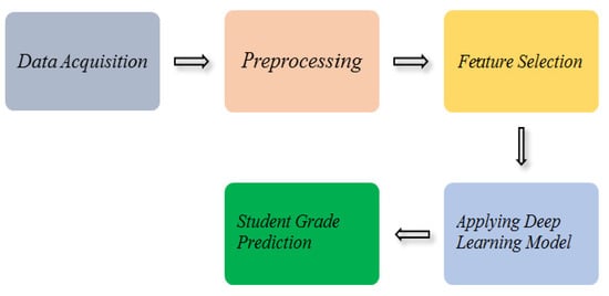
Figure 1. Overview of Student Grade Prediction System.

3.1. Acquisition of Dataset

We acquired the student grade prediction dataset from the UCI Machine Learning Repository [17]. The acquired student dataset contains 33 attributes with 1044 records (see Table 1).

Table 1. Attribute Detail of Student Dataset.

Figure	Feature Name	Description
F1	School_f	Name of student’s school
F2	Sex_f	Student’s gender
F3	Age_f	Age of student
F4	Address_f	Home address type of student’s
F5	Famsize_f	Size of family
F6	Pstatus_f	Cohabitation status of parent
F7	Medu_f	Student’s mother’s education
F8	Fedu_f	Student’s father’s education
SF9	Mjob_f	Student’s mother’s job
F10	Fjob_f	Student’s father’s job
F11	Reason_f	Why school was chosen
F12	Guardian_f	Guardian of student
F13	Traveltime_f	Travel time from home to school
F14	Studytime_f	Study time in a week
F15	Failures_f	Number of class failures in past
F16	Schoolsup_f	Additional educational support
F17	Famsup_f	Educational support from family
F18	Paid_F	Extra paid classes within the course subject
F19	Activities_f	Extra-curricular activities
F20	Nursery_f	Attending nursery school
F21	Higher_f	Desire of taking higher education
F22	Internet_f	Internet facility at home
F23	Romantic_f	Have a romantic relationship
F24	Famrel_f	Family relationships quality
F25	Freetime_f	After school free time
F26	Gout_f	Going outside with friends
F27	Dalc_f	Alcohol usage at daytime
F28	Walc_f	Alcohol usage at weekend
F29	Health_f	Recent health status
F30	Absences_f	Absences from school
F31	G1_f	Grade of the first period (numeric: from 0 to 20)
F32	G2 _f	Grade of the second period (numeric: from 0 to 20)
F33	G3_f (target)	Grade of final period (numeric: from 0 to 6)

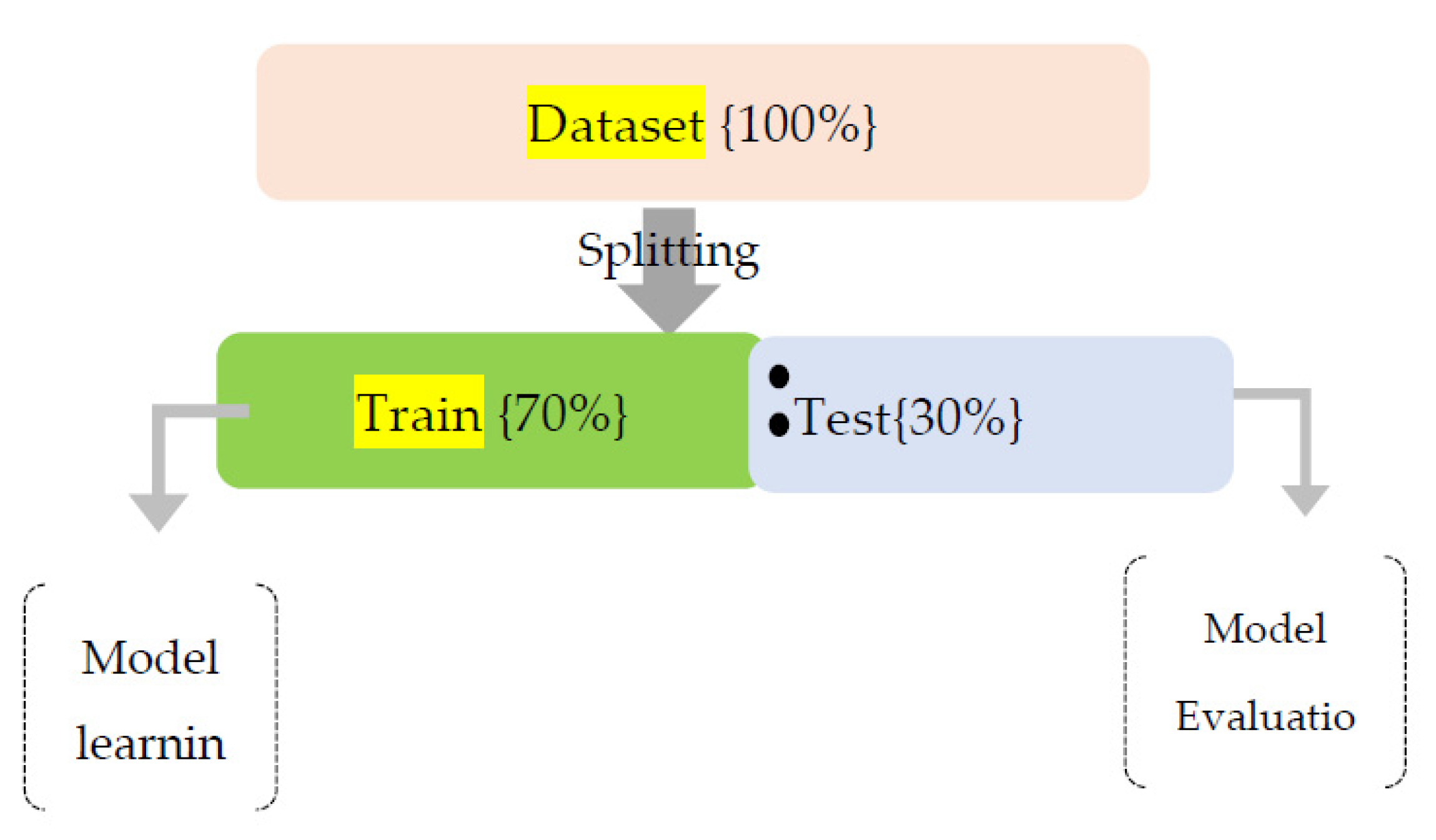
Splitting of Dataset

Splitting of a dataset into two partitions is performed with a ratio of 70:30 using the SKlearntrain_test_split function , [18] as shown in Figure 2.

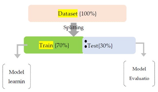
Figure 2. Split Ratio of Training and Test Dataset.

3.2. Data Preprocessing

To develop an effective predictive model, it is essential to apply data preprocessing steps, because data in the raw format degrades the performance of the machine learning classifiers. The acquired dataset is in a raw format containing skewed data. We performed the following preprocessing steps:

Transformation of textual data to numeric form: In this step of preprocessing, textual data is transformed to numerical format by using the SklearnLabelEncoder [19]. Table 2 shows a partial listing of such data.

Table 2. Numeric Conversion of Textual data.

School_f	Sex_f	Age_f	Address_f	Famsize_f	…….	G1_f	G2_f	G3_f (Target Feature)
0	0	18	1	0	…….	0	11	11
0	0	17	1	0	…….	9	11	11
0	0	15	1	1	…….	12	13	12

Transformation of categorical variables into a numeric form: There are certain attributes, also called categorical variables, which contain multiple values for a single variable. Such attributes need to be converted into the numerical format in order to perform experiments on the supervised learning classifier (machine/deep learning) effectively. We applied the Pandas library function, namely “Categorical’ to convert the categorical variables into the numerical format by assigning a separate numeric value to each attribute [20]. For example, the target class variable “G3_f” takes numeric values in the range of 0 to 6 (0:A1, 1:A, 2:B, 3:C, 4:D, 5:E, 6:F). For more simplicity, what we have conducted is that we simply calculated the percentage for each record and each grade by dividing the individual value of each grade by the total number of grades. i.e., 20 [0–19], and stored the percentage to the corresponding column, e.g., all the percentages of G1, G2, G3 (Target Class) are stored in PercentageG1, PercentageG2, PercentageG3, respectively, and we conducted this because we aimed to classify 20 grades into simple 7 grades. So, we obtained the above-mentioned columns, GradesG1, GradesG2, and GradesG3.

3.3. Feature Selection

Feature Selection (FS) aims at including the significant features from the dataset by discarding the insignificant attributes. Resultantly, the selected features have a significant impact on the prediction capability of the model [21].

There are different methods for FS: (i) information gain [22], (ii) principal component analysis (Li et al. 2018), (iii) recursive feature elimination [23], (iv) extra tree classifier [24], and (v) Chi-Square test. In this work, we choose to apply the Chi-square test to select features, motivated by the prior study [25] where the authors applied it for the selection of relevant features and received an improved performance in supervised learning.

It is a statistical technique to determine whether the occurrence of a specific class and occurrence of a specific feature is independent or not by evaluating the association of categorical variables with respect to target variables.

The Chi-Square test is formulated as follows:

$$X_c^2={\displaystyle \sum }\frac{{\left(Oi-Ei\right)}^2}{Ei}$$

(1)

where c = degree of freedom, O = observed value (observation in class), and E = expected observation in class (i) if there was no relationship between the feature and the target variables.

The Chi-Square value $x^2$ can be calculated from feature variables and target variables in order to select those attributes which have a strong correlation with the target/predicted class.

We applied the Chi-Square test on the student grated prediction dataset to select the desired attributes having more dependency with the target class. We used the Sklearn library package available in Python with the integration of SelectKBest and Chi2 function to perform relevant feature selection. A relevant feature is one whose likelihood contains more association with the target class. The top 10 most relevant features are selected on the basis of their association and dependency with the target class. The relevant attributes are then arranged in order with high relevant frequency scores on the top. Table 3 contains the top 12 relevant/optimal features and their relevancy score.

Table 3. Optimal Feature Set.

S.No	Relevant Features	Relevancy Score
1	G2_f	418.452
2	G1_f	333.616
3	Absences_f	294.363
4	Failures_f	255.779
5	Mjob_f	34.889
6	Fjob_f	34.143
7	Medu_f	33.568
8	Fedu_f	32.369
9	Schoolsup_f	21.756
10	Studytime_f	19.575
11	Health_f	14.519

3.4. System Overview

The proposed approach (see Figure 3) for predicting student grades from the given 32 features using deep learning model contains several layers such as the (i) Embedding Layer, (ii) Bidirectional LSTM Layer, (v) Attention Layer and (vi) Prediction using Output Layer.

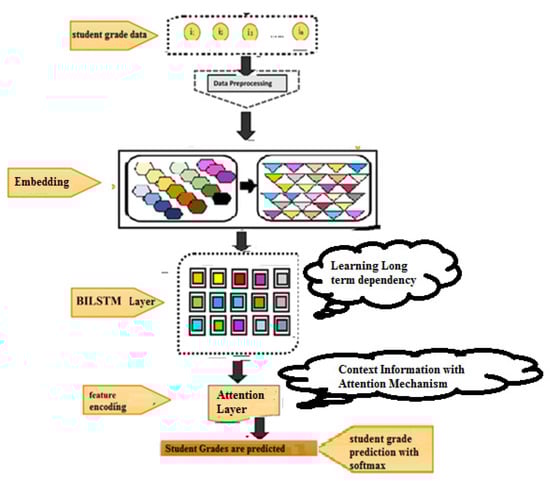
Figure 3. Overview of the Proposed System.

(i)

Embedding Layer: The input data is transformed into index sequences, and after that, the index sequences are converted to a vector of features by using the embedding layer implemented in Keras. Resultantly, a vector of real values is generated as output.

(ii)

Bidirectional LSTM Layer: the aim of adding the BiLSTM layer is to learn long-term dependency and to exploit the contextual information from the backward as well as the forward directions.

(iii)

Attention Layer: the attention layer emphasizes the important feature from the contextual information obtained from the BiLSTM layer, which can further improve the classification accuracy [26].

(iv)

Prediction using Output Layer: finally, the softmax activation function is applied to predict student grades between (0–6) [27].

4. Detailed Architecture

4.1. Model Design

An attention-based BiLSTM model (See Figure 4) is proposed for the predicting of student grades from historical academic data. It is comprised of the following layers: (i) Embedding, (ii) BILSTM, (iii) Attention, and (iv) Output.

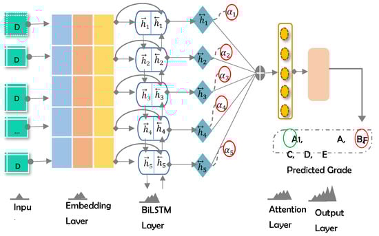
Figure 4. Design of the Proposed Model.

4.1.1. Embedding Layer

Consider an input data comprised of n values: $D=\left[d_1, d_2,d_3,\dots \dots .d_n\right]$. Each data chunk $di$ is converted into a continuous-valued vector, where $d_i\in {ℝ}^{d}d$ show the dimension of the data embedding. In this work, we used Keras embedding layer³² to produce the data embedding vector. Now the embedding layer generates a feature matrix $F\in {ℝ}^{d\mathrm{x}n}$, where $n$ shows the length of the input data. This input representation is passed to the next layer.

4.1.2. Bidirectional Layer

The authors of [28] introduced BiLSTM for extending the one-direction LSTM, while the BiLSTM contains a second hidden layer, and the hidden links flow within the opposite temporal sequence. Consequently, the model has the ability to exploit the information in two directions, namely, past and future [29]. In the proposed work, BiLSTM is introduced to retain the information of past and future

The BiLSTM is composed of two hidden layers namely forwards LSTM, and backward LSTM. The explanation of both the layers is given below.

First hidden layer-forward LSTM: The processing of the sequence during this layer is conducted from the left towards right direction through the concatenation of two inputs, such as past input ‘$h_{t-1}$’, as well as present input ‘$a_t$’. Given an input series: $a_1$,$a_2$,$a_3$,…, $a_{y-1}$, the result sequence of forwarding LSTM is ‘$\overrightarrow{h}$’.

Second hidden layer-backward LSTM: The processing of sequence during this layer is conducted from right towards left direction through the concatenation of two inputs, such as future input ‘$h_{t+1}$’, as well as present input ‘$x_t$’. Given an input series: $a_{y+1}$,…,$a_2$,$a_3$,$a_1$, the result sequence of backward LSTM is ‘$\overleftarrow{h}$’.

The illustration of left (forward) context is ‘$\overrightarrow{h}$’, and the illustration of right (backward) context is ‘$\overleftarrow{h}$’, where both these representations ($\overrightarrow{h}$, $\overleftarrow{h}$) are combined, that creates a new review matrix $H=\left[h_1,h_2,h_3,\mathrm{\dots },h_c\right]$, where $H ϵ {ℛ}^{c\times m}$. The merging of both the left and the right outcome is performed using an element-wise addition, mathematically (Equation (2)) define as follows:

$$\overleftrightarrow{h }=\overrightarrow{h}\oplus \overleftarrow{h}$$

(2)

The final review matrix ($\overleftrightarrow{h }$) is then forward to the classification layer of the neural network. The mathematical calculations regarding the first hidden layer (forward LSTM) (Equations (3)–(8)) and the second hidden layer (backward LSTM) (Equations (9)–(14)) are illustrated as below.

Equations of the first hidden layer (forward LSTM):

$$i_t=\sigma \left(W_i\left[h_{t-1},a_t\right]+b_i\right)$$

(3)

$$f_t=\sigma \left(W_f\left[h_{t-1},a_t\right]+b_f\right)$$

(4)

$$o_t=\sigma \left(W_o\left[h_{t-1},a_t\right]+b_o\right)$$

(5)

$$c{\sim }_t=\tau \left(W_c\left[h_{t-1},a_t\right]+b_c\right)$$

(6)

$$c_t=f_t\circ c_{t-1}+i_t\circ c{\sim }_t$$

(7)

$$\overrightarrow{h_t}=o_t\circ \tau \left(c_t\right)$$

(8)

Equations of the second hidden layer (backward LSTM):

$$i_t=\sigma \left(W_i\left[h_{t+1},a_t\right]+b_i\right)$$

(9)

$$f_t=\sigma \left(W_f\left[h_{t+1},a_t\right]+b_f\right)$$

(10)

$$o_t=\sigma \left(W_o\left[h_{t+1},a_t\right]+b_o\right)$$

(11)

$$c{\sim }_t=\tau \left(W_c\left[h_{t+1},a_t\right]+b_c\right)$$

(12)

$$c_t=f_t\circ c_{t+1}+i_t\circ c{\sim }_t$$

(13)

$$\overleftarrow{h_t}=o_t\circ \tau \left(c_t\right)$$

(14)

Here, the terms $i_t$, $f_t$, $o_t$ are used to represent three different gates, namely, input, forget, and output gate, $\sigma$ represents the sigmoid function, $\tau$ represents a tangent function, $\circ$ shows the Hamdard product, $W_i$, $W_f$, $W_o$, and $W_c$ represent the weight metrics regarding the input gate, forget gate, output gate, and cell state. The $h_{t-1}$, and $h_{t+1}$ denotes the past and future hidden states, $a_t$ denotes the present input, $b_i$, $b_f$, $b_o$, $b_c$ denotes the bias vector, $c{\sim }_t$ represents the candidate value, $c_t$ shows cell state, while $c_{t-1}$ and $c_{t+1}$ illustrates the past and future cell state. Now, the final review representation generated at the BiLSTM is forwarded to the next layer of the neural network. In Table 4, the mathematical terms used during the context information extraction strategy are listed.

Table 4. Mathematical Terms for Context Information Extraction Strategy.

Mathematical Terms	Definition
$a_t$	Present input
$h_{t-1}$	Past input
$h_{t+1}$	Future input
$H$	New review matrix created through BiLSTM
$\overleftrightarrow{h }$	Final review matrix ($\overrightarrow{h_t}+\overleftarrow{h_t}$)
$i_t$, $f_t$, $o_t$	Input, forget, and output gate
$c{\sim }_t$, $c_t$, $c_{t-1}$, $c_{t+1}$	Candidate value, cell state, past and future cell state
$b_i$, $b_f$, $b_o$, $b_c$	Bias vectors
$W_i$, $W_f$, $W_o$, and $W_c$	Weight metrics regarding input gate, forget gate, output gate, and cell state.
$\circ$, $\sigma$, $\tau$	Hamdard product, sigmoid, and tangent function

4.1.3. Attention Layer

The attention layer aims to focus on words having a decisive role in prediction. A set of computations used in this layer are formulated as follows:

$$n_i=tanh\left(W{h}_i+b\right)$$

(15)

$$c_i=softmax\left(m_i\right)$$

(16)

$$v={{\displaystyle \sum }}_{j=1}^k{c}_i{h}_i$$

(17)

The output of the predecessor layer is represented by $h_i$, bias is depicted by b, W shows weight, $c$ depicts attention weight for each data element in the input sequence of student grade prediction sequence, c and $v$ shows the attention vector.

4.1.4. Output Layer

The student grade (A1, A, B, C, D, E, F) is predicted at the output layer using the sigmoid function. It is computed as follows:

$$z=sigmoid\left(y \right)$$

(18)

5. Applied Example

In this section, we describe different mathematical operations to predict a student’s final grade from a given student data. A detailed representation of these operations is abstracted below.

5.1. Data Preparation for DL Model

In this step, student data are prepared for the DL model, which is received from the feature selection module. For this purpose, we used Keras tokenizer, which converts the given data into an array of indexes, i.e., $\left[1, 2,3,4,5\right],$ which is then passed to the embedding layer of the DL model.

5.2. Embedding Layer

It transforms each index in the student data sequence to a stream-valued vector. For example, the student data “absences” with [1] index is converted to a vector embedding [0.4 0.6 0.3 0.2]. As a result, we received matrix embeddings as depicted in Table 5.

Table 5. A Sample of Vector Embedding.

Index	Vector Embedding
1	[0.4 0.6 0.3 0.2]
2	[0.8 0.9 0.2 0.6]
3	[0.2 0.5 0.6 0.4]
4	[0.7 0.1 0.3 0.4]
5	[0.1 0.3 0.5 0.7]

5.3. Dropout Layer

To resolve the issue of overfitting, the dropout layer is introduced after the embedding phase. A threshold of 0.5 is used to randomly deactivate the neurons in the embedding layer.

5.4. BiLSTM Layer

The BiLSTM layer performs processing on the input received from the dropout layer and produces an encoded outcome. The computation of the forward LSTM (Equations (3)–(8)) and the backward LSTM (Equations (9)–(14)) are described as follows:

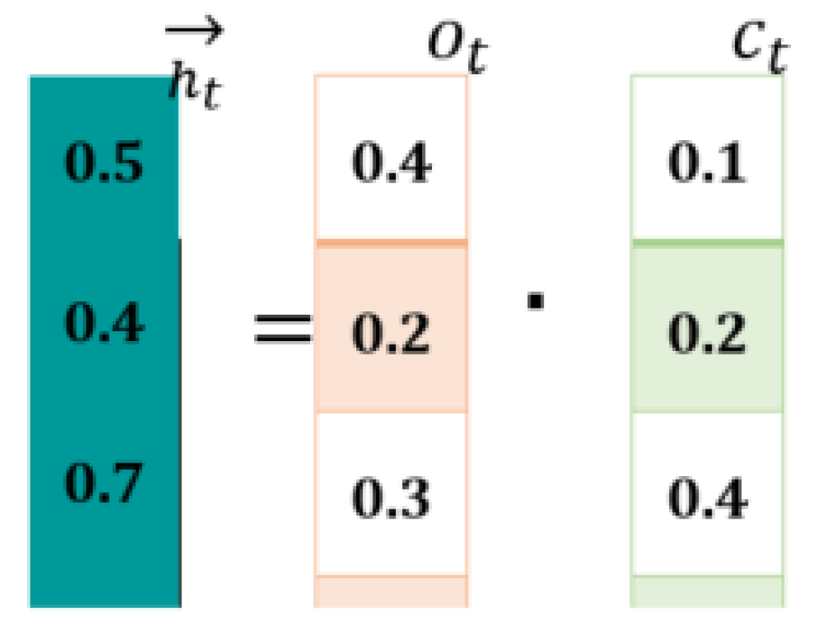
Computations at Forward LSTM (First Hidden Layer): The forward LSTM generates a hidden state “$\overrightarrow{h}$” by combining the current ($i_t$) and previous state ($h_{t-1}$). For this purpose, it makes use of Equations (3)–(8). Figure 5 shows computations.

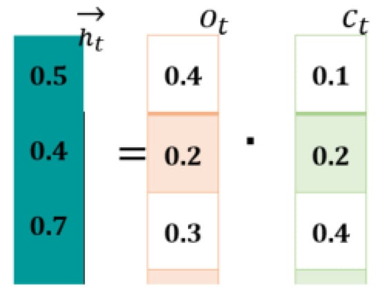
Figure 5. Forward LSTM Computation.

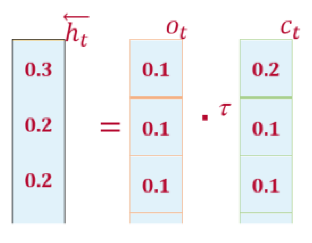
Computations at Backward LSTM (Second Hidden Layer): The backward LSTM generates hidden state “$\overleftarrow{h}$” by combining the current ($i_t$) and next state ($h_{t+1}$). For this purpose, it makes use of Equations (7)–(12). Now we put in the values in Equation (14) as shown in Figure 6.

Figure 6. Backward LSTM Computation.

The BiLSTM Outcome: to generate the final outcome of the BiLSTM (“$\overleftrightarrow{h}$”), Equation (2) is applied to perform the cell-wise addition of “$\overrightarrow{h}$” and “$\overleftarrow{h}$, shown as follows (Figure 7):

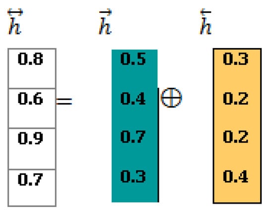
Figure 7. BiLSTM Final Representation.

The information encoded by BiLSTM is input into the attention layer for further processing.

5.5. Attention Layer

The attention layer applies Equation (15) for computing the importance of student data as follows:

$$n_1=\tau anh\left[0.8 0.6 0.9 0.7\right]\left[\begin{array}{c}0.6\\ 0.8\\ 0.9\\ 0.7\end{array}\right]+\left[0.2\right]=\left[0.5\right]$$

(19)

In same way, $n2=0.4, n3=0.3, n4=0.2$, and $n5=0.5$.

In the next step, Equation (16) is applied to compute attention weights, shown as follows:

$$c_{1=e^{0.5}/e^{0.5}+e^{0.2}+e^{0.3}+e^{0.4}+e^{0.5}=0.3}$$

(20)

In the same way, we computed,$c2=0.4, c3=0.2, c4=0.5, and c5=0.3$.

Finally, a weighted summation of each $h_i$ and $c_i$ is aggregated using Equation (17).

$$\mathsf{\gamma }\left[\begin{array}{c}\begin{array}{c}0.59\\ 0.66\\ 0.57\end{array}\\ 0.74\end{array}\right]=c1\ast \left[\begin{array}{c}\begin{array}{c}0.8\\ 0.6\\ 0.9\end{array}\\ 0.7\end{array}\right]+c2\ast \left[\begin{array}{c}\begin{array}{c}0.6\\ 0.1\\ 0.3\end{array}\\ 0.2\end{array}\right]+c3\ast \left[\begin{array}{c}\begin{array}{c}0.9\\ 0.4\\ 0.9\end{array}\\ 0.5\end{array}\right]+c4\ast \left[\begin{array}{c}\begin{array}{c}0.5\\ 0.1\\ 0.7\end{array}\\ 0.4\end{array}\right]+c5\ast \left[\begin{array}{c}\begin{array}{c}0.7\\ 0.6\\ 0.5\end{array}\\ 0.8\end{array}\right]$$

(21)

In this way, an attention vector is obtained for the final prediction.

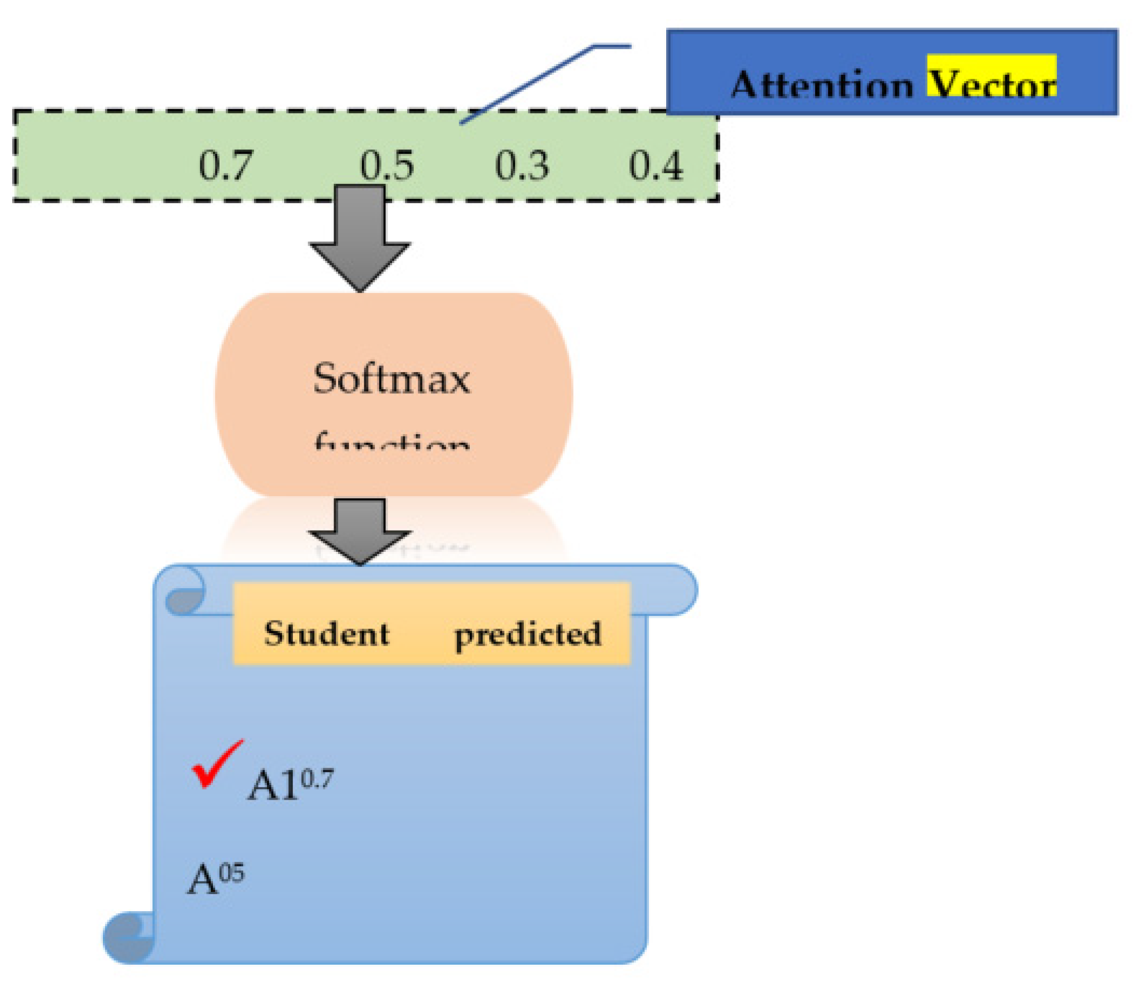
5.6. Prediction Layer

The attention vector received from the prior layer (attention layer) is given to the prediction layer, where we apply the softmax function to calculate the probability of student grade (G3) classes, such as “A1”, “A”, “B”, “C”, “D”, “E”, and “F. For this purpose, the input is calculated using Equation (19) as follows:

$$X_j={{\displaystyle \sum }}_{j=1}^k{w}_{j}l+b$$

(22)

Using Equation (22), input is calculated as follows:

$$x1=0.8, x2=0.3,\dots ..x7=0.7$$

The probability of x is calculated using the softmax function as follows:

$$\sigma \left(x_i\right)=\frac{e^{x_i}}{{{\displaystyle \sum }}_{k=1}^7{e}^{x_k}}$$

For student grade class label=“A1”

$$\mathrm{put} i=1: \sigma \left(x_1\right)=e^1/e^1+e^2+\cdots e^7=0.7$$

For student grade class label=“A”

$$\mathrm{put} \mathrm{I}=2:\sigma \left(x_2\right)=e^2/e^1+e^2+\cdots e^7=0.5$$

For student grade class label=“B”

$$\mathrm{put} \mathrm{I}=3:\sigma \left(x_3\right)=e^3/e^1+e^2+\cdots e^7=0.3$$

For student grade class label=“F”

$$\mathrm{put} \mathrm{I}=1:\sigma \left(x_7\right)=e^7/e^1+e^2+\cdots e^7=0.1$$

The aforementioned calculations show that the “A1” student grade class obtained the probability with the highest value among other student grade classes. Therefore, from the given student data stream “…………….”, the predicted grade is “A1” (see Figure 8).

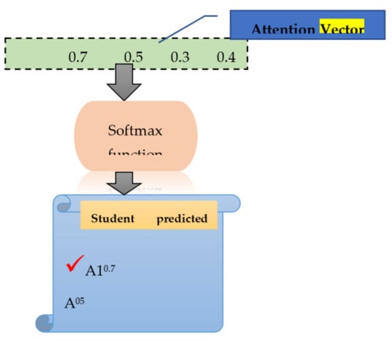
Figure 8. Student Grade Prediction using the softmax Function.

The pseudocode steps of the proposed approach for student grade prediction are shown in Algorithm 1.

Algorithm 1. Pseudocode of Proposed Student Grade Prediction Model.

Input: Student performance labelled dataset D as csv file.

II. Spilt into train (Strain, NRtrain)-test (Stest, NStest) using Scikit learn.

III. Build the vocabulary to map integer to student data

IV. Transform each student data stream into sequence of integers.

V. Procedure Attention-based BiLSTM model(Strain, NStrain)

Initialize max_features, embed_dim, input_length, classes, NEpoch, batch_size, BiLSTM units

Split Dataset into Train, Test

Initialze Sequential function

Generate Embeddings

Adding Dropout Layer

Add Bidirectional LSTM layer

Add Attention Layer

Incorporate Softmax function

Compile Function

Evaluate model on Test dataOutput: return grade

End Procedure

5.7. User Interface of the Proposed System

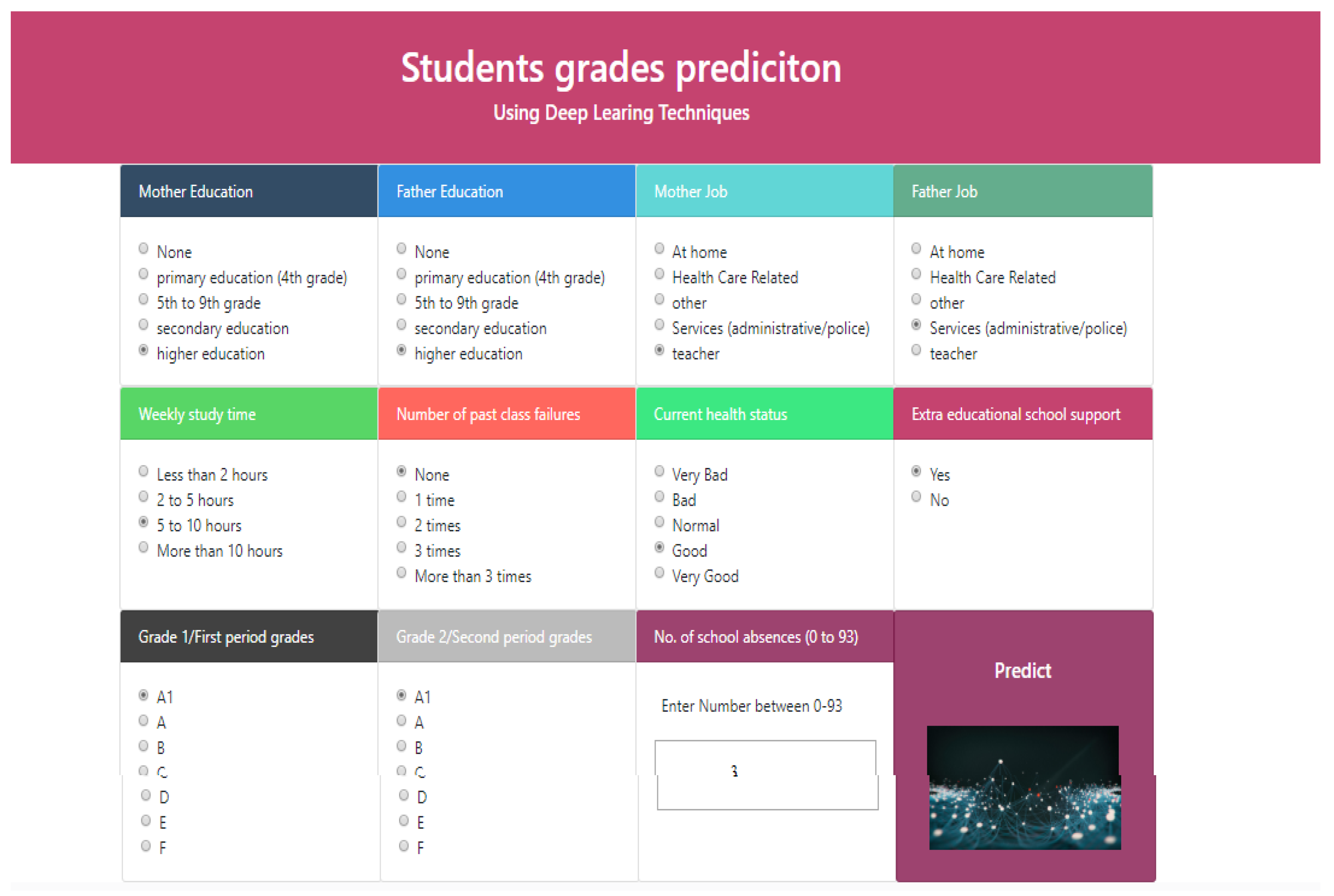
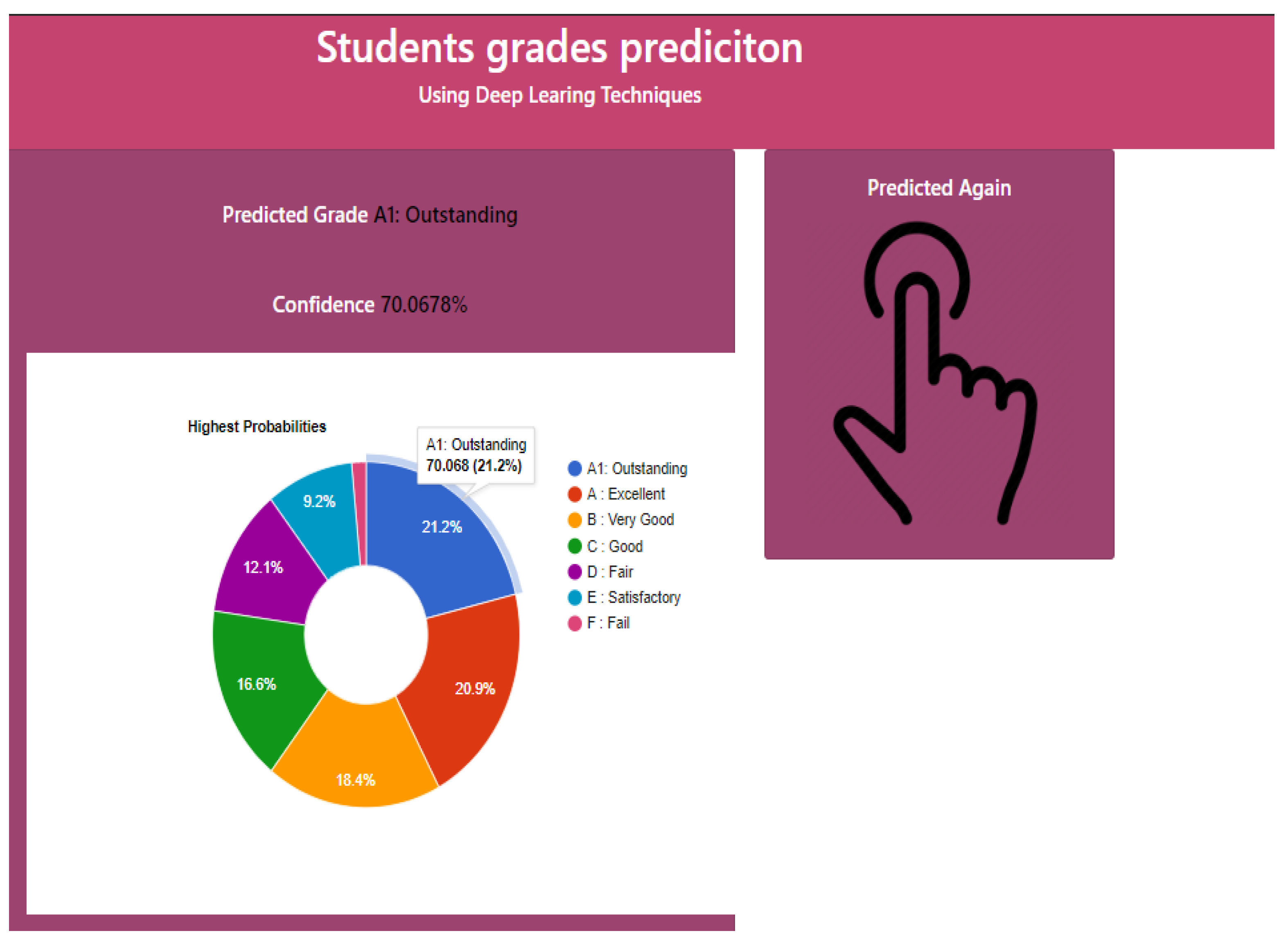
To predict student grade from given student academic performance-related data, we developed a user-friendly web interface using a Python-based Flask environment, and the trained deep learning model is deployed using the Keras library. The front end (main page) of the web application is shown in Figure 9. An online user can enter the student data (Figure 9), then after pressing the predict button, an output is displayed as “A1: Outstanding”, “A: Excellent”, “B: Very Good”, “C: Good”, “D: fair”, “E: satisfactory” or “F: Fail” with a predicted confidence rate. Figure 10 shows that the predicted grade for a sample set of parameters is “A1”.

Figure 9. Home Page for Student Grade Prediction Using Deep Learning.

Figure 10. Grade Prediction Output Screen.

6. Results and Discussion

We have performed the following experiments: (i) using all 33 features as input and G3 (final grade) as the target variable, (ii) using top rank features (see Table 3) selected as an input, and G3 column (final grade) as the predicted output variable.

6.1. Experiments

Different experiments are performed on the benchmark dataset and the results are reported in this section.

6.1.1. To Apply a Deep Learning Model, Namely the Attention-Based BiLSTM Model for Predicting Student Final Grade from Historical Academic Data

To select the most optimal attention-based BiLSTM model for predicting student grades, we have performed a tuning of hyperparameters. Table 6 shows the hyperparameters setting for the proposed model. The different hyperparameters related to the model are as follows: Filter No, kernel_size, pool_size, BiLSTM unit size, batch_size, Activation function, and optimizer.

Table 6. Proposed Model Parameter Tuning.

Model Layers	Hyperparameters Values
Embedding Layer
max_features	2000
Size of vocabulary	6000, 7000, 12,000, 60,000, 80,000
Size of input vector	53, 60
random_state	2, 7, 8, 9
Dimension of embedding vector	128, 140, 170, 185, 210, 230
Dropout Layer
Unit Size	0.5
Attention Layer
Units	150
BiLSTM Layer
Unit Sizes	20, 60, 90, 110, 150, 200
Others
batch_size	32
Activation	Softmax
Optimizer	RMSprop

Table 7 shows different versions of the attention-based BiLSTM by keeping the size of the batch as either 32 or 64, whereas the unit size of the BiLSTM and the dimensions of embedding are altered. It is obvious that the model exhibited better performance with a unit size of 60, Dimension of Embedding = 128, and size of batch = 32. Furthermore, it is obvious that the accuracy of the model keeps on improving when the BiLSTM unit size increases and the dimension of embedding decreases.

Table 7. Different Versions of Variations of Attention-based BiLSTM model.

Model	Unit Size of BiLSTM	Dimension of Embedding	Size of Batch
Attention-based BiLSTM-1	10	230	64
Attention-based BiLSTM-2	20	210	32
Attention-based BiLSTM-3	26	185	64
Attention-based BiLSTM-4	30	170	32
Attention-based BiLSTM-5	50	140	64
Attention-based BiLSTM-6	60	128	32

The experimental results of different attention-based BiLSTM models (with feature selection) by adjusting the hyperparameters are presented in Table 8.

Table 8. Performance Measure of Attention-based BiLSTM Models (with Feature Selection).

Name of Model	Acc. (%)	P (%)	R (%)	F (%)	Test Loss
Attention-based BiLSTM-1	84.39	0.85	0.84	0.84	0.84
Attention-based BiLSTM-2	85.13	0.85	0.85	0.85	0.34
Attention-based BiLSTM-3	85.81	0.86	0.86	0.86	0.32
Attention-based BiLSTM-4	86.74	0.87	0.87	0.87	0.32
Attention-based BiLSTM-5	87.17	0.87	0.87	0.87	0.31
Attention-based BiLSTM-6	90.16	0.90	0.90	0.90	0.24

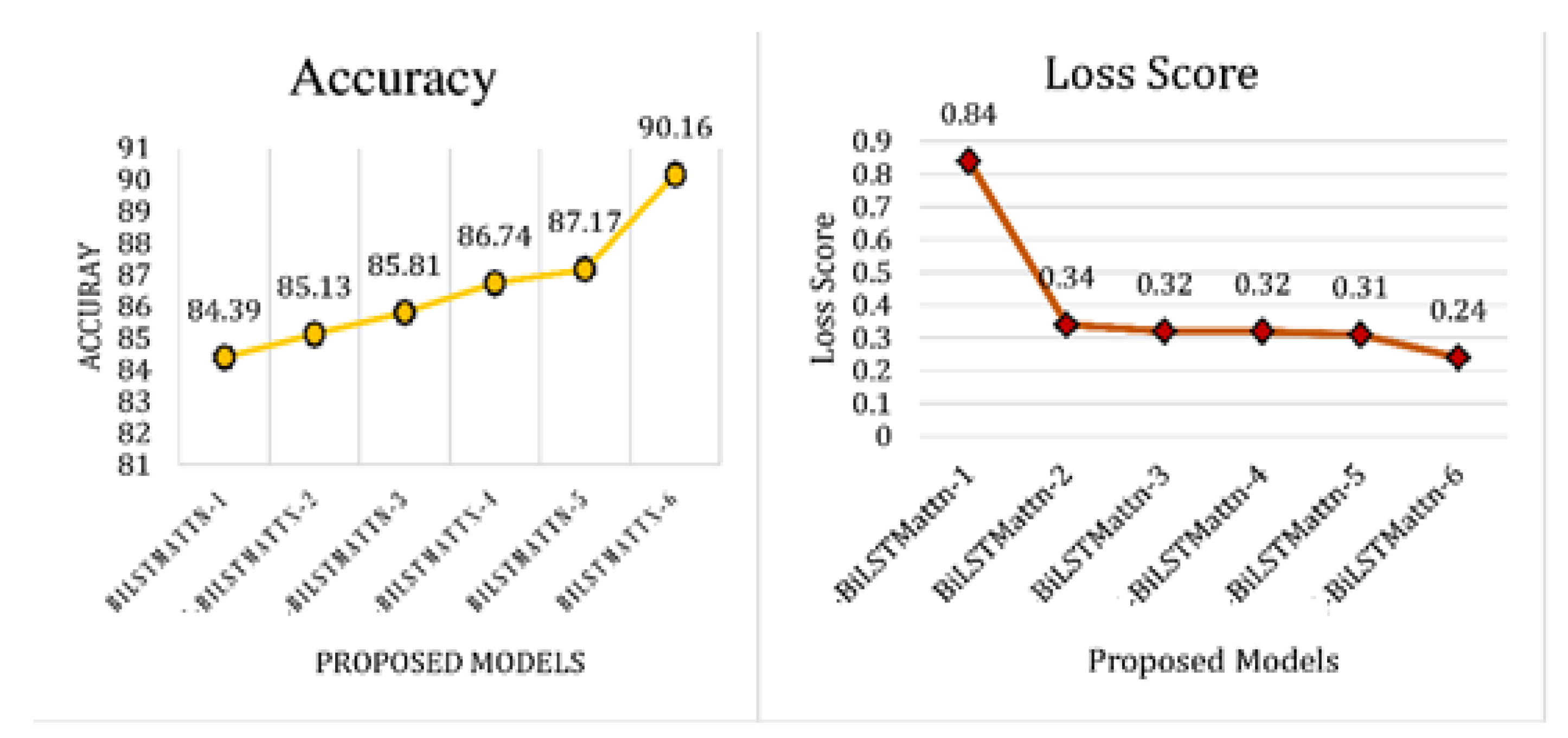
After performing the aforementioned experimentation, it is observed that the model performs best with hyperparameters values (Filter No:16., kernel_size:3, pool_size:2, BiLSTM_Unit Size:20, Batch size:32,), whereas activation and optimizer values are kept the same as the change in these values do not affect the performance of the model. In Table 8, we report the performance metrics of all six attention-based BiLSTM models in terms of precision, recall, f-measure, and accuracy. The experimental results depict that model-6 of the attention-based BiLSTM achieved the highest accuracy of 90.16%, precision (0.90), recall (0.90), f-score (0.90) with regard to the other models.

In Figure 11, it is also noted that with the increase in the accuracy, the loss score of the model is decreasing, which shows that as the model’s accuracy has improved and the errors are decreasing.

Figure 11. Accuracy and Loss Score Comparison of Attention-based BiLSTM Models.

The experimental results of different attention-based BiLSTM models (without feature selection) by adjusting the hyperparameters are presented in Table 2.

6.1.2. To Evaluate the Performance of the Proposed Attention-Based BiLSTM over the Traditional Machine Learning Techniques

To address this research objective, we implemented various machine learning models, such as K-NN, MNB, SVM, LR, and RF to predict a student’s grade from the given student’s performance data. The results presented in Table 9 show that the proposed attention-based BiLSTM model performed better than the classical machine learning classifiers.

Table 9. Proposed Model Comparison with respect to ML Classifier.

Method	Acc. (%)	P (%)	R (%)	F-Score (%)
Machine Learning classifiers
Support vector machine (SVM)	70.79	0.80	0.71	0.68
Logistic Regression (LR)	81.67	0.83	0.82	0.81
Naïve Bayes (NB)	82. 21	0.85	0.83	0.82
K-Nearest Neighbor (KNN)	84.55	0.85	0.85	0.84
Random Forest (RF)	85.33	0.85	0. 85	0. 85
Proposed Method
Attention-based BiLSTM (with feature selection)	90.16	0.90	0.90	0.90
Attention-based BiLSTM (without feature selection)	88.46	0.88	0.88	0.88

6.2. To Evaluate the Performance of the Proposed Technique for the Student Grade Prediction with Respect to the State-of-the-Art Methods and Other Deep Learning Techniques

We evaluated the effectiveness of the proposed model with other deep learning models, namely, RNN, CNN, LSTM, BiLSTM, and the baseline study utilized the machine learning model. The results reported in Table 10 depict that the proposed model performed better (precision, recall, f-score, and accuracy) than other models. Table 10 illustrates that the proposed deep learning attention-based BiLSTM achieved the best results than the baseline (machine learning) study, as well as the other deep learning techniques, such as RNN, CNN, LSTM, BiLSTM.

Table 10. Proposed Method with respect to DL Models.

Method	Acc. (%)	P (%)	R (%)	F-Score (%)
Deep Learning Techniques
Recurrent Neural Network (RNN)	81.64	0.85	0.82	0.81
Convolutional Neural Network (CNN)	85.56	0.86	0.86	0.86
Long Short-Term Memory (LSTM)	86.16	0.88	0.86	0.86
Bidirectional Long Short-Term Memory (BiLSTM)	88.88	0.89	0.89	0.89
Machine Learning (SVM) (Imran et al. 2019)	80.38	43.94	39.53	39.70
Proposed Method
Attention-based BiLSTM (with feature selection)	90.16	0.90	0.90	0.90
Attention-based BiLSTM (without feature selection)	88.46	0.88	0.88	0.88

6.3. Employing Significance Test

In this work, we performed two experiments to approve the statistical significance of the proposed attention-based BiLSTM model using word embedding features with a conventional machine learning classifier using traditional features.

We have a carried out an investigation that the performance difference of both the proposed attention-based BiLSTM and the ML-based random forest are statistically distinct and do not take place fortuitously. We randomly selected 186 records reviews of student data, in which each of the data records are predicted using the attention-based BiLSTM and RF models. The results are reported in Table 11, So, in order to validate the null hypothesis, McNemar’s test is used.

Table 11. Computing McNemar Statistical Test.

	RF Correctly Classified	RF Misclassified	Total
Attention-based BiLSTM correctly predicted	80	31	111
Attention-based BiLSTM misclassified	15	60	75
	95	91	186

H₀: both models have the same error rate for student grade prediction.

H_A: the two models have different error rates for student grade prediction.

In Equation (14), McNemar’s test statistics are formulated, i.e., Chi-Squared having the degree of freedom 1.

$$x={(c_{01}-c_{10})}^2/c_{01}+c_{10}$$

(23)

In Table 11, the result of the McNemar statistical test is presented.

Table 12 shows the summary statistics of Chi-Square, p-value, and degree of freedom.

Table 12. Summary Statistics of McNemar’s Test.

p-Value	0.027
McNemar’s Chi-Squared statistic	4.9
Degrees of freedom	1

The Chi-Squared value is 4.9 and the two-tailed p-value is 0.027 with one degree of freedom.

Results reported in Table 13 show that the proposed system outperformed baseline methods in terms of improved accuracy, precision, recall, and f-score. Our proposed BiLSTM with an attention-mechanism technique resulted in an accuracy of 88.46% without feature selection. The performance of the proposed system further improves when feature selection is incorporated. It achieves an accuracy of 90.16%. These results are much better, as compared to existing baseline studies including [30,31].

Table 13. Comparison of Proposed Method with Baseline Methods.

Method	Technique	Acc. (%)	P (%)	R (%)	F-Score (%)
Sultana et al. (2019)	MLP-a	84.88	86.48	82.24	81.65
Imran et al. (2019)	SVM	80.38	73.94	69.53	69.70
Proposed method	Attention-based BiLSTM (with feature selection)	90.16	0.90	0.90	0.90
Proposed method	Attention-based BiLSTM (without feature selection)	88.46	0.88	0.88	0.88

We obtained good results when comparing studies as (i). BiLSTM with an attention mechanism is used which usually shows good results in classification tasks (ii). Feature selection is performed in our work. It is assumed that feature selection improves accuracy. It is clear that our proposed deep learning model is showing improved performance with the inclusion of feature selection.

6.4. Discussion

The prediction results for the random forest classifier using the traditional feature are presented in Table 9. It is noted that the RF with a traditional features representation scheme exhibits poor performance as compared to our proposed model in terms of precision, recall, f-measure, and accuracy.

In the next experiment, the performance of the attention-based BiLSTM model using embedding-based features is measured, which depicts improved results (Table 9) in terms of better precision (0.59), recall (0.59), f-measure (0.58), and accuracy (0.58).

The aforementioned significant test verifies that a significant difference is found among the two models: the proposed attention-based BiLSTM and the machine learning-based random forest model.

Table 11 shows that number of discordant pairs is 46, which means that the two classifiers perform differently for incorrect prediction. After applying McNemar’s test, the two-tailed p-value is 0.027, with a degree of freedom 1, and the Chi-Squared value is 4.9. So, the alternate hypothesis is accepted, i.e., the two models have different error rates for personality recognition and rejecting the null hypothesis because 0.027< 0.5.

7. Conclusions and Future Work

It is an important task to predict student performance (grades) from the historical academic data. The proposed approach is performed different tasks, namely, (i) data acquisition, (ii) preprocessing, (iii) feature selection, and (iv) applying a deep learning model for student grade prediction. Experiments are conducted on the students’ benchmark dataset. After performing the necessary preprocessing steps, feature selection is performed to select the most relevant features with a high ranking in the statistical result. Finally, an attention-based BiLSTM model is applied for student grade prediction. The experimentation of the proposed approach is conducted on the students’ benchmark dataset. The experimental results show that the proposed model yielded the best results when compared with the baseline work. The limitations of this study include the dataset confined to a single domain (benchmark study). Furthermore, only significant features are considered for prediction, whereas the consideration of other features such as student’s social and cultural characteristics, and time spent to complete a special task, may result in better performance. In the future, multiple datasets need to be investigated with more variations of fused deep learning models.

References

- UN. Sustainable Development Goals; UN: New York, NY, USA, 2019. [Google Scholar]
- Tsiakmaki, M.; Kostopoulos, G.; Kotsiantis, S.; Ragos, O. Transfer learning from deep neural networks for predicting student performance. Appl. Sci. 2020, 10, 2145. [Google Scholar] [CrossRef] [Green Version]
- Sin, K.; Muthu, L. Application of Big Data in Education Data Mining and Learning Analytics—A Literature Review. ICTACT 2015, 5, 1035–1049. [Google Scholar] [CrossRef]
- Mizumoto, T.; Ouchi, H.; Isobe, Y.; Reisert, P.; Nagata, R.; Sekine, S.; Inui, K. Analytic Score Prediction and Justification Identification in Automated Short Answer Scoring. In Proceedings of the Fourteenth Workshop on Innovative Use of NLP for Building Educational Applications, Florence, Italy, 2 August 2019; pp. 316–325. [Google Scholar] [CrossRef]
- Polyzou, A.; Karypis, G. Grade prediction with models specific to students and courses. Int. J. Data Sci. Anal. 2016, 2, 159–171. [Google Scholar] [CrossRef] [Green Version]
- Thai-nghe, N.; Drumond, L.; Krohn-grimberghe, A.; Schmidt-thieme, L. Recommender System for Predicting Student Performance. Procedia Comput. Sci. 2010, 1, 2811–2819. [Google Scholar] [CrossRef] [Green Version]
- Khan, B.; Khiyal, M.S.H.; Khattak, M.D. Final Grade Prediction of Secondary School Student using Decision Tree. Int. J. Comput. Appl. 2015, 115, 32–36. [Google Scholar] [CrossRef]
- Hussain, S.; Khan, M.Q. Student-Performulator: Predicting Students’ Academic Performance at Secondary and Intermediate Level Using Machine Learning. Ann. Data Sci. 2021. [Google Scholar] [CrossRef]
- Dahdouh, K.; Dakkak, A.; Oughdir, L.; Ibriz, A. Large-scale e-learning recommender system based on Spark and Hadoop. J. Big Data 2019, 6, 2. [Google Scholar] [CrossRef]
- Liu, S.; He, T.; Dai, J. A survey of CRF algorithm based knowledge extraction of elementary mathematics in Chinese. Mob. Netw. Appl. 2021, 1–13. [Google Scholar] [CrossRef]
- Lu, O.H.T.; Huang, A.Y.Q.; Huang, J.C.H.; Lin, A.J.Q.; Ogata, H.; Yang, S.J.H. Applying learning analytics for the early prediction of students’ academic performance in blended learning. Educ. Technol. Soc. 2018, 21, 220–232. [Google Scholar]
- Rahman, T.; Zhou, Z.; Ning, H. Energy Efficient and Accurate Tracking and Detection of Continuous Objects in Wireless Sensor Networks. In Proceedings of the 2018 IEEE International Conference on Smart Internet of Things (SmartIoT), Xi’an, China, 17–19 August 2018; pp. 210–215. [Google Scholar] [CrossRef]
- Xiang, J.; Zhou, Z.; Shu, L.; Rahman, T.; Wang, Q. A Mechanism Filling Sensing Holes for Detecting the Boundary of Continuous Objects in Hybrid Sparse Wireless Sensor Networks. IEEE Access 2017, 5, 7922–7935. [Google Scholar] [CrossRef]
- Rajendran, V.; Fang, M.H.; Guzman, G.N.D.; Lesniewski, T.; Mahlik, S.; Grinberg, M.; Leniec, G.; Kaczmarek, S.M.; Lin, Y.S.; Lu, K.M.; et al. Super broadband near-infrared phosphors with high radiant flux as future light sources for spectroscopy applications. ACS Energy Lett. 2018, 3, 2679–2684. [Google Scholar] [CrossRef]
- Sun, L.; Hu, L.; Zhou, D. Improving 7th-Graders’ Computational Thinking Skills Through Unplugged Programming Activities: A Study on the Influence of Multiple Factors. Think. Ski. Creat. 2021, 42, 100926. [Google Scholar] [CrossRef]
- Paura, L.; Arhipova, I. Cause Analysis of Students’ Dropout Rate in Higher Education Study Program. Procedia-Soc. Behav. Sci. 2014, 109, 1282–1286. [Google Scholar] [CrossRef] [Green Version]
- Musleh, M.; Ouzzani, M.; Tang, N.; Doan, A.H. CoClean: Collaborative Data Cleaning. In Proceedings of the 2020 ACM SIGMOD International Conference on Management of Data (SIGMOD ’20), Portland, OR, USA, 14–19 June 2020; Association for Computing Machinery: New York, NY, USA, 2020; pp. 2757–2760. [Google Scholar] [CrossRef]
- Massey, C.T. Mining Research. Colliery Guard. Redhill 1987, 235, 50–54. [Google Scholar] [CrossRef]
- Ahmad, S.; Asghar, M.Z.; Alotaibi, F.M.; Awan, I. Detection and classification of social media-based extremist affiliations using sentiment analysis techniques. Hum.-Cent. Comput. Inf. Sci. 2019, 9, 24. [Google Scholar] [CrossRef] [Green Version]
- Khattak, F.K.; Jeblee, S.; Pou-Prom, C.; Abdalla, M.; Meaney, C.; Rudzicz, F. A survey of word embeddings for clinical text. J. Biomed. Inform. X 2019, 4, 100057. [Google Scholar] [CrossRef]
- Ahmad, H.; Asghar, M.Z.; Khan, A.S.; Habib, A. A systematic literature review of personality trait classification from textual content. Open Comput. Sci. 2020, 10, 175–193. [Google Scholar] [CrossRef]
- Uǧuz, H. A two-stage feature selection method for text categorization by using information gain, principal component analysis and genetic algorithm. Knowl.-Based Syst. 2011, 24, 1024–1032. [Google Scholar] [CrossRef]
- Lahoti, P.; Gummadi, K.P.; Weikum, G. IFair: Learning individually fair data representations for algorithmic decision making. In Proceedings of the 2019 IEEE 35th International Conference on Data Engineering (ICDE), Macao, China, 8–11 April 2019; pp. 1334–1345. [Google Scholar] [CrossRef] [Green Version]
- Brownlee, W.J.; Altmann, D.R.; Prados, F.; Miszkiel, K.A.; Eshaghi, A.; Gandini Wheeler-Kingshott, C.A.; Barkhof, F.; Ciccarelli, O. Early imaging predictors of long-term outcomes in relapse-onset multiple sclerosis. Brain 2019, 142, 2276–2287. [Google Scholar] [CrossRef]
- Najeeb, R.F.; Dhannoon, B.N. Classification for Intrusion Detection with Different Feature Selection Methods: A Survey (2014–2016). Int. J. Adv. Res. Comput. Sci. Softw. Eng. 2017, 7, 305–311. [Google Scholar] [CrossRef]
- Zhang, W.; Liu, Y.; Guo, Z. Approaching high-performance potassium-ion batteries via advanced design strategies and engineering. Sci. Adv. 2019, 5, eaav7412. [Google Scholar] [CrossRef] [PubMed] [Green Version]
- Sun, J.; Jin, R.; Ma, X.; Park, J.Y.; Sohn, K.A.; Chung, T.S. Gated Convolutional Neural Networks for Text Classification. Lect. Notes Electr. Eng. 2021, 715, 309–316. [Google Scholar] [CrossRef]
- Schuster, M.; Paliwal, K.K. Bidirectional recurrent neural networks. IEEE Trans. Signal Process. 1997, 45, 2673–2681. [Google Scholar] [CrossRef] [Green Version]
- Zhou, P.; Qi, Z.; Zheng, S.; Xu, J.; Bao, H.; Xu, B. Text classification improved by integrating bidirectional LSTM with two-dimensional max pooling. In Proceedings of the COLING 2016, the 26th International Conference on Computational Linguistics: Technical Papers, Osaka, Japan, 11–17 December 2016; Volume 2, pp. 3485–3495. [Google Scholar]
- Imran, M.; Latif, S.; Mehmood, D.; Shah, M.S. Student academic performance prediction using supervised learning techniques. Int. J. Emerg. Technol. Learn. 2019, 14, 92–104. [Google Scholar] [CrossRef] [Green Version]
- Sultana, J.; Rani, M.U.; Farquad, M.A.H. Student’s performance prediction using deep learning and data mining methods. Int. J. Recent Technol. Eng. 2019, 8, 1018–1021. [Google Scholar]
Publisher’s Note: MDPI stays neutral with regard to jurisdictional claims in published maps and institutional affiliations. |
© 2021 by the authors. Licensee MDPI, Basel, Switzerland. This article is an open access article distributed under the terms and conditions of the Creative Commons Attribution (CC BY) license (https://creativecommons.org/licenses/by/4.0/).