Abstract
Blade geometry is an important design parameter that influences global wind turbine energy harvesting performances. The geometric characteristics of the blade profile are obtained by determining the distribution of the chord and twist angle for each blade section. In order to maximize the wind energy production, implying a maximum lift-to-drag ratio for each wind speed, this distribution should be optimized. This paper presents a methodology to numerically determine the change in the twist angle by introducing a range of pitch angles for the maximum power coefficient case. The obtained pitch values were distributed from the root to the tip of blade. The results prove that the power coefficient increases for wind speeds greater than the rated point, which improves the yearly production of energy by 5% compared to the reference case.
1. Introduction
Wind energy represents a very important and largely used green energy source. The extraction of this energy is based on wind turbines, which can have many types of designs, among which it is remarked that the horizontal-axis wind turbine represents the most commonly used one. Specifically, a horizontal-axis wind turbine generally consists of a three-blade rotor that is further connected to an electrical generator. This type of wind turbine can extract over 40% of the wind kinetic energy [1]. The efficiency of this process is strongly related to the blade geometry, the profile of each section having a specific aerodynamic shape that allows rotation of the blade under the wind flow by generating a tangential force. The intensity of this force is related to the lift-to-drag ratio, which has a specific value for each wind speed [2].
1.1. Literature Review
Liu et al. [3] determined a new optimal blade shape for a fixed-speed wind turbine. Its chord and twist distributions are linearized, aiming to harvest the maximum energy at all wind speed values. The results demonstrated that the new design enables an increased annual energy production (AEP) compared to the preliminary design. It was highlighted that the AEP increase is related to the rated wind speed value.
Burton et al. [2] gave a linearized chord distribution as a straight line passing through points that carry 70% and 90% of the theoretical distribution of the chord to reduce the blade shape. Their results fell within the limits of Betz’s ideal model.
Capellaro et al. [4] established an iterative method to determine the optimal twist distribution that ensures the torsional deflection blade equilibrium and aims to maximize the power production. Their results showed a significant increase in the AEP.
Sessarego et al. [5] developed a computer program to obtain the optimal output parameters for small-scale wind turbine blades (where it has the best starting time, low noise, high power coefficient, and low blade mass). The program is based on the genetic algorithm and starts from BEM theory, beam theory, and the IEC61400-2 standard.
Hassanzadeh et al. [6] presented an optimization method to define the optimal aerodynamic blade shape. This method relies on the genetic algorithm using the Viterna approach as a post-stall model. Their implementation showed a high capability to predict the performance of the wind turbine. In addition, the blade shape determined by this method gave an increase in AEP, reaching up to 8.5%.
Yang et al. [7] presented a new method of optimization based on an improved genetic algorithm (NSGA-II), aiming to define the low-mass blade geometry and increase the AEP. Their simulation was made with STAR-CCM+ and was validated based on blade element momentum (BEM) theory. The results defined a new blade geometry that can increase the AEP by 2.48%, having a low mass ratio of 5.52 compared to the initial blade.
Tahani et al. [8] defined the optimal linearized chord and twist angle distribution for a large-scale wind turbine. It was proved that the linearized distribution based on the point of linear slope enables a higher efficiency. The four airfoils Riso-A1-21, Riso-A1-18, S809, S814, and DU 93-W-210 were used. The results showed that the point corresponded to 60% to 64% and 30% to 37% of the blade length, providing the best slope line of the chord and twist distribution.
Lee et al. [9] introduced the realistic conditions to optimize a range of aerodynamics of wind blade design. The objective function and the design parameters relationship were determined by the statistical methodology of a response surface. Their results gave increases of 8.7% in efficiency and about 7% in AEP, where the rated speed advanced 4% compared to the initial value.
Rahgozar et al. [10] presented a method of investigation based on genetic algorithms. It aims to maximize the power coefficient and minimize the starting time of small wind turbines. Four design cases were studied, both linear and nonlinear chord and twist distributions and both mixed. The results showed that the best configuration was both the linear chord and twist design, which gave the best starting time and maximum power output.
Moradtabrizi et al. [11] employed the genetic algorithm method to define the optimal blade geometry. Their work aimed to reduce the cost of production with high energy production. The geometry analysis was based on the Bezier curve. The NREL 5 MW blade was taken as a reference model. Their results showed acceptable energy production with losses reaching 3% compared to the reference model, but a gain of 15% was registered in the total cost of production.
Yang [12] addressed the effect of linearized blade geometry on the aerodynamic performance in which an optimization algorithm was established based on linearization parameters such as the chord and twist angle. This algorithm was applied for multiple tip speed ratios to identify the best aerodynamic performance. The result demonstrated that the increase in chord slope gives high performance with low wind speed. A lower slope increases the performance with high wind speed. For the twist angle effect, it has considerable results with low wind speed.
Kaya [13] introduced a new study based on the CFD method and using the k-e turbulence model. In this approach, a machine learning method and support vector regression were used, aiming to define the optimal distribution of the twist angle for high generated torque. The results gave an optimal twist with a three-node cubic spline distribution, evaluating a 10% torque increase with the NREL VI blade model, much higher with NREL II.
Mendez et al. [14] presented a method of determining the chord and twist distribution for maximizing the mean power produced. In this case, the assumptions of optimal attack angle that corresponded to a high lift-to-drag ratio was avoided. On the other hand, blade element theory was used to reduce the computational cost, where it was validated with the experimental data of the Riso test wind turbine, and where the prediction of mean power was carried out using the genetic algorithm. The method gave good results under the stall point.
Xudong et al. [15] gave a method to optimize the wind turbine, aiming to reduce the cost of power production. The method is a combination of the aeroelastic model and dynamic model of analysis with 11 degrees of freedom, where the BEM theory was introduced by considering the new developed tip loss factor. The model results were compared with the experimental data of the MEXICO 25 kW experimental rotor, the Tjæreborg 2 MW rotor, and the NREL 5 MW wind turbine. For Tjæreborg 2 MW, a reduction in chord of 16% at a radial position of 15 m was registered, and for NREL 5 MW, it was 8.2% at a radial position of 40 m. For MEXICO 25 kW, there was no change in chord distribution. In addition, the cost of power reduced to 3.4%, 1.1%, and 2.6% respectively.
Schubel et al. [16] presented a review paper about wind blade design, where the relationship of aerodynamic performance and structural performance was recapitulated by determining the contribution of airfoil types and the best attack angle, as opposed to the aerodynamic, centrifugal, gyroscopic and gravity loads. This aimed to demonstrate the large uses of the horizontal-axis wind turbine, which presented an efficient model.
Derakhshan et al. [17] developed a method to optimize the blade shape. This method based on an artificial bee colony (ABC) coupled by an artificial neural network was applied on the NREL phase VI by using the results of aerodynamic analysis performed via CFD and BEM theory, compared and validated by experimental data. The results showed that the best optimized blade shape parameters gave an increase of 8.58% in power output.
Utsch et al. [18] gave a revised study of the aerodynamic optimization of wind turbines considering the drag effect. The analysis was carried out by using blade element momentum theory where the optimization problem was taken as a nonlinear programming problem. The optimization analysis was based on quality and inequality constraints by using Lagrange’s multipliers. Their results gave a diagram of the operation conditions that corresponded to the maximum power coefficient for each drag-to-lift ratio.
Nair et al. [19] gave a new blade design solution that aimed to increase the efficiency of wind turbines. This solution summarized adding microtabs to the blade body. Three blade models were studied: the first one with two microtabs; the second with one microtab; and the last without. The results obtained by using CATIA and ANSYS software showed that the blades with two microtabs was the best model, with a high power coefficient.
Abdelsalam et al. [20] gave a comparison study between a classical model of blade shape and new linearized model. The classical blade had a nonlinear chord distribution from 0.12 to 0.04 m and a nonlinear distribution of twist from 27° to 4.22°. The linearized model was defined by many stages where the values of the chord and twist fixed at the tip and values at the root were varied with the variation in linear slope. The best shape (G8) had a chord linear distribution from 0.09 to 0.04 m and a twist linear distribution from 15° to 4.22°. The model was manufactured and tested experimentally in an open air-jet test rig. The results showed that the new model of the blade reduced 26% of the volume compared to the classical blade model. On the other hand, it maintained the value of the power coefficient above 0.4 as the nonlinear model in a large range of tip speed ratios. However, it reached this power coefficient value at 5 m/s, unlike the nonlinear model, which reached it at 6 m/s.
1.2. Research Objectives
The efficiency of wind turbines is first related to the design parameters, being directly influenced by their variation. In this research, the values corresponding to the lift-to-drag ratio varied under the design parameters such as the chord distribution and twist angle, where the twist was considered as an angular coordinate of each blade section. The correlation between design parameter and output efficiency determines the scientific community to focus on finding the best distribution of these parameters that provides the optimal blade shape. Thus, an investigation method based on BEM theory, with a new blade design with a corrected twist angle, is proposed in this paper. The correction was performed by the addition of a range of optimal pitch angles, where the value of the pitch angle was determined for each wind speed value within the operational range. The numerical test of new designs was carried out in three installation sites. These sites have mean wind speeds equal to 5, 6, and 7 m/s. The performance evaluation was carried out based on the analysis of power, power coefficient, and AEP results.
2. Performance of Wind Turbine
2.1. Blade Element Momentum Theory
The analysis of wind turbines is based on the combination of analytical momentum theory and blade element theory [21]. This combination, known as BEM theory, was established by Gluaert to determine the driving torque and thrust force (defined in Equations (1) and (2), respectively) for each blade section, as defined by [21,22]. In reference to Figure 1, a and a′ are the axial and tangential induction factors, respectively, Ω represents the wind turbine rotation speed, V1 is the wind speed, and r is the radial position.
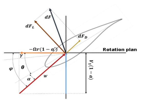
Figure 1.
Wind speeds and forces system configuration at blade section.
According to the second theory of analysis, which is based on the aerodynamic flow, the torque and thrust are defined by [21,22]:
where B is the blade number, Cl and Cd are the lift and drag coefficient, respectively, and W represents the relative wind speed determined by [21,22]:
where F is the Prandtl tip and root correction coefficient, and φ is the flow angle. They are defined, respectively, by [21,22]:
where R is the wind turbine radius, Rh is the blade root radius, and λr is the speed ratio at each radial position, determined by [21,22]:
In Equations (3) and (4), Cr presents the chord and is defined depending on the Betz model by the following expression [21,22]:
where λ is the global speed ratio [14,15]:
On the other hand, from Figure 1, the twist angle is:
where γ is the pitch angle, and α is the attack angle.
Based on the Betz model, the optimal twist distribution defines when the axial induction factor equals 1/3 with no radial induction. It can be expressed based on Equations (7) and (11) with the inclusion of the value of induction factors by [21]:
According to the combination of Equations (1)–(4), the axial and tangential induction factors are defined as follows [21,22]:
where σ presents the solidity [21,22]:
The flow effect on the rotor expressed by the thrust coefficient is determined by [14,15]:
In the case of high induction, where the axial induction factor is greater than 0.4, the thrust effect will be higher, and the basic Equation (16) cannot express the real thrust. In this context, various experimental studies have been conducted to correct this instability case. In 2005, Buhl gave a new expression of the thrust coefficient where the axial induction factor is greater than 0.4 [23]. It is expressed by:
where Cn and Ct are the normal force and tangential force coefficients, respectively, and they are defined by [21,22]:
The Cl and Cd coefficients are determined by the XFOIL software for the range of −10° to 15°. Outside this range, they are determined by the Viterna et al. model as follows [3,24]:
For , the lift and the drag coefficients are, respectively, defined by [24]:
where the constant B1 is determined by [24]:
presents the maximal drag coefficient. AR is the aspect ratio of the profile and is determined by:
The constants B2, A1, and A2 are obtained from [24]:
αstall and Cdstall are the values of attack angles and drag coefficient at the stall point.
The power of the wind turbine can be determined from [21]:
The performance determined by the power coefficient can be calculated from [21]:
2.2. The Annual Energy Production
The AEP of a wind turbine is the total power achieved over a year. It is related to the frequency of wind speed at the site. It is defined by the following expression [3]:
where η is the mechanical conversion efficiency and is equal to 0.9. ρ is the air density and f is the frequency of each wind speed at the site. Weibull or Ryleigh models can express this frequency. These distribution models are based on the scale factor C and shape factor k. In this work, the frequency distribution expressed by the Ryleigh model, which presents a specific case of Weibull with a value of shape factor k, equals 2, as presented in the following [25]:
where C is the scale factor and is defined by [25]:
where Vm is the mean wind speed of the installation site.
3. Methodology of Optimization
3.1. Preliminary Design
Based on the previous mathematical model of BEM that is summarized by the flowchart presented in Figure 2, a MATLAB programming code has been established to analyze the performance of each case. A high induction correction is introduced under the Buhl model [23]. Otherwise, the Cl and Cd variation is determined by the Viterna model [24], as presented in Figure 3. The reference design of the wind turbine consists of 7.5 m blades with a NACA23015 as a profile section, which reaches the maximum lift-to-drag coefficient at an attack angle of 10°, with a Reynolds number equal to 1 × 10⁶. At this angle, the lift and drag are equal to 1.22 and 0.01, respectively [26]. The blades design adopted had a tip speed ratio to 6. The design parameters, such as twist angle (θ) and chord (Cr), are presented in Figure 4 and listed in Table 1. These parameters are evaluated based on Equations (9) and (12), where the pitch angle (γ) is equal to 0°. The first and second section are estimated as the root section, which have a circular shape with a diameter equal to 50% of the value of the chord of the third section and null twist angle.
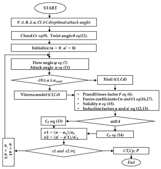
Figure 2.
BEM flowchart.
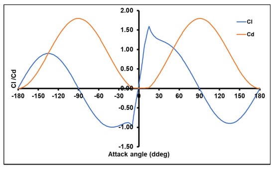
Figure 3.
Viterna lift and drag variation of NACA23015.
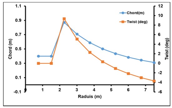
Figure 4.
Chord and twist angle distribution.

Table 1.
Blade geometry parameters.
3.2. Pitch Variation
In this work, the reference model was studied in three sites, which have mean wind speed values of 5, 6, and 7 m/s. The rotation speeds adopting the design tip speed ratio were 38, 45, and 53 RPM, respectively. The test was performed in the range from −15 to +15 of the pitch angle. The AEP was calculated based on the Rayleigh wind speed distribution of the three sites, as shown in Figure 5.
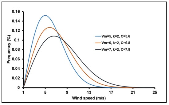
Figure 5.
Rayleigh wind speed frequency distribution.
Figure 6, Figure 7 and Figure 8 of the three sites show that the power coefficient becomes maximum at a tight range of pitch angles. This range can overlap for consecutive wind speed values. The pitch angle corresponds to the maximum power coefficient increase from the cut-in wind speed value to the mean wind speed value. Otherwise, it decreases from the mean wind speed to the cutout wind speed.
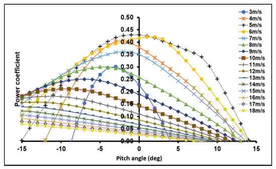
Figure 6.
Power coefficient vs. pitch angle (5 m/s model).
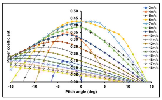
Figure 7.
Power coefficient vs. pitch angle (6 m/s model).
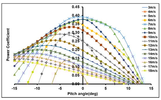
Figure 8.
Power coefficient vs. pitch angle (7 m/s model).
3.3. Polynomial Pitch Distribution
After assessing the range of pitch angles for which the power coefficient reaches the maximum, each mean wind speed is shown in Figure 5, Figure 6, Figure 7 and Figure 8. The variation in pitch angle was quasi-linear from the cut-in wind speed to the mean wind speed, as well as from the mean wind speed to the cutout wind speed. This variation adapted mathematically to a range of whole speed values (Figure 9), where the pitch ranges varied under the following expressions:
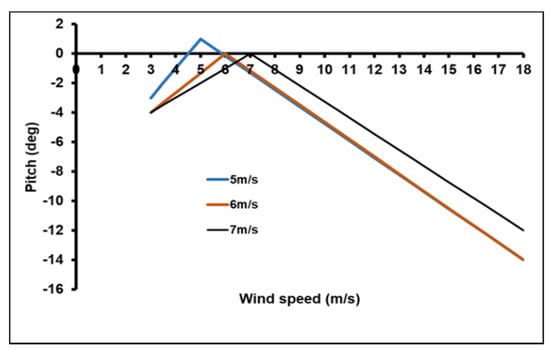
Figure 9.
Optimal pitch angle variation.
From the cut-in wind speed value to the mean wind speed value:
- First site (Vm = 5 m/s)
- Second site (Vm = 6 m/s)
- Third site (Vm = 7 m/s)
From the mean wind speed value to cut-out wind speed value:
- First site (Vm = 5 m/s)
- Second site (Vm = 6 m/s)
- Third site (Vm = 7 m/s)
3.4. Optimized Design
From the preview section, the new pitch values (depicted in Figure 9) were added to the twist angle values of the preliminary model. The addition may be via the reverse way, from the root to the tip of blade with respect to the root sections, conserving their value. The new twist angle is presented in Figure 10.
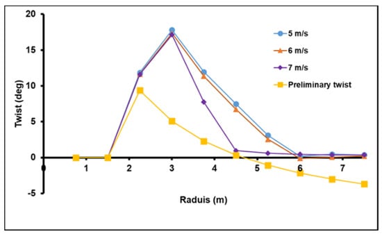
Figure 10.
New twist angle distribution.
4. Results and Discussion
Starting from the results of the BEM MATLAB programming code, the modified models were tested in the three installation sites that have mean wind speeds of 5, 6, and 7 m/s. Two cases were taken into account to evaluate the performance of the proposed models. The first case corresponds to a wind speed value greater than the design value (15 m/s). The second case has a lower wind speed than the design value (5 m/s). The results were then compared with the preliminary model. The attack angle, and lift and drag coefficients had similar values in the three sites, as presented in Figure 11, Figure 12 and Figure 13, because the design adopted the same value of wind speed ratio, showing the variation in these quantities for wind speeds of 5 and 15 m/s. In Figure 11, the results show a decrease in the attack angle compared to the reference model in the three cases of study. This decrease was due to the twist correction, which made the attack angle come close to the optimal value corresponding to the wind speed of 15 m/s. However, in the case of 5 m/s wind speed, the decrease in attack angle determined an attack angle far from the optimal value. That is explained by the variations in the lift and drag coefficient, respectively, presented in Figure 12 and Figure 13.
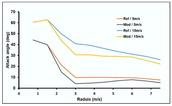
Figure 11.
The variation in attack angle.
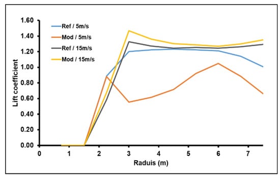
Figure 12.
The variation in lift coefficient.
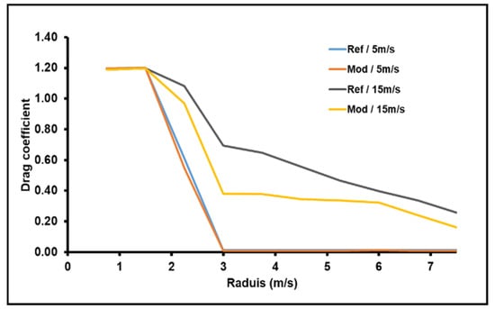
Figure 13.
The variation in drag coefficient.
It is noticed that the variation in lift coefficient increased under the correction of the twist blade angle. This increase was just in the case of the 15 m/s wind speed. Contrariwise, the rotor registered a lower lift in the case of operating under a wind speed of 5 m/s. In terms of the drag coefficient, the result showed no change with a wind speed of 5 m/s and a decrease with 15 m/s. This decrease was accompanied by an increase in the lift-to-drag coefficient. As a consequence, the rotation torque increased, causing the rotor to harvest the maximum of kinetic energy.
Figure 14, Figure 15 and Figure 16 clearly express the previous remarks, where the power coefficient of modified models took lower values compared to the preliminary model (Figure 14a, Figure 15a and Figure 16a). These lower values were registered with wind speed values less than the rated point, where the rated points were 8, 10, and 12 m/s of the models of 5, 6, and 7 m/s, respectively. The mean decreases in power coefficient were registered up to 18% for the models of 5 and 6 m/s and was 2% with the 7 m/s model. These lower values are related to the lift decrease at lower wind speeds (Figure 12). After the rated point, the power coefficient of the modified model registered higher values compared to the reference model. This improvement was due to the augmentation of the lift increasing the wind speeds (Figure 12). This is clearer in terms of the produced power presented in Figure 14b, Figure 15b and Figure 16b, where the power of modified models took high values up to 50% with the 5 and 6 m/s models and 20% with the 7 m/s model.
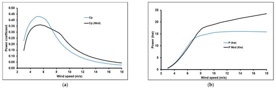
Figure 14.
The variations in (a) power coefficient and (b) power for the mean wind speed case of 5 m/s.
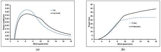
Figure 15.
The variations in (a) power coefficient and (b) power for the mean wind speed case of 6 m/s.
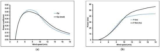
Figure 16.
The variations in (a) power coefficient and (b) power for the mean wind speed case of 7 m/s.
The results were validated by using the FAST package. The simulation was performed for both cases. The cases of 5 and 15 m/s wind speeds were tested, and the results showed more accurate values with the first analysis, where the modified models had high power coefficients (RotCp) at 15 m/s with the preliminary model, but was the opposite at 5 m/s (Figure 17, Figure 18 and Figure 19).
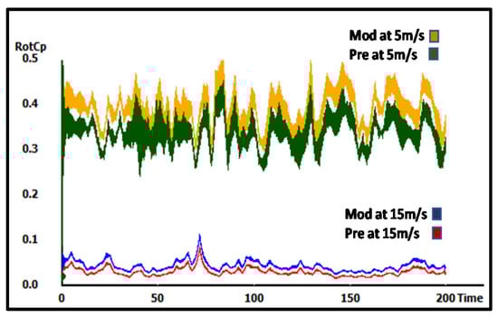
Figure 17.
The FAST power coefficient results of 5 m/s mean wind speed model.
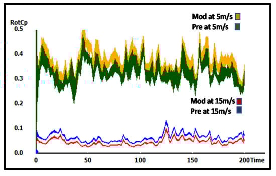
Figure 18.
The FAST power coefficient results of 6 m/s mean wind speed model.
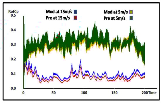
Figure 19.
The FAST power coefficient results of 7 m/s mean wind speed model.
The final comparative evaluation of the new designs was carried out by means of the AEP, as shown in Figure 20. The results proved that the modified model registered an increase of up to 5% in the energy production compared to the reference model, as displayed in Figure 21.
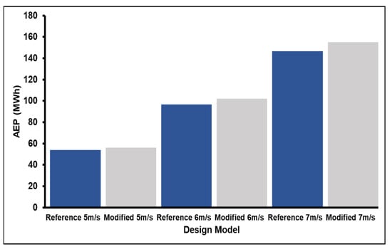
Figure 20.
The annual energy production variation.
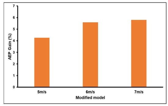
Figure 21.
The gain in annual energy production.
5. Conclusions
The twist angle is an important parameter that has a direct influence on wind turbines performances, also defining the blade twisting geometry distribution. Moreover, the pitch angle determines the blade optimal angular position for a high power coefficient. This paper proposed a new twist angle correction method, which is based on the best pitch angle range for each wind speed. In this case, three preliminary blade designs were tested in three sites, which have mean wind speeds of 5, 6, and 7 m/s. The pitch angle varied from −15° to 15°. The performance analysis was made by means of a BEM MATLAB code, developed for this application. The optimal pitch angle distribution from the cut-in wind speed to the cutout value was mathematically modelled, varying the optimal pitch values from the cut-in to cutout wind speed. These intermediary results were added to the preliminary twist angle from the root to the tip reversely, where the optimal pitch angle corresponds to the cut-in wind speed added to the twist angle at the tip of blade and to the cut-out wind speed added to the twist angle at the root section. The analysis resulted in a new twisted blade design that showed an increased lift for a wind speed value greater than the rated value. Thus, the power coefficient increased, determining an increase in the AEP that can reach up to 5% compared with the preliminary model.
Author Contributions
Conceptualization, M.D., M.H. and S.D.; methodology, M.D., M.H. and S.D.; software, M.D. and M.H.; validation, S.D.; formal analysis, M.D., M.H. and S.D.; investigation, M.D. and M.H.; resources, M.D., M.H. and S.D.; data curation, M.D. and M.H.; writing—original draft preparation, M.D. and M.H.; writing—review and editing, D.-A.C.; visualization, M.D. and M.H.; funding acquisition, G.L. and D.-A.C. All authors have read and agreed to the published version of the manuscript.
Funding
This research received no external funding.
Acknowledgments
The authors would like to acknowledge Ouahiba Guerri, director of wind division, and Hafida Daaou Nedjari, a chief of the aerodynamic team, for their advice that enhanced the quality of this work.
Conflicts of Interest
The authors declare no conflict of interest.
Nomenclature
| α | Attack angle (deg). |
| γ | Pitch angle (deg). |
| θ | Twist angle (deg). |
| σ | Solidity. |
| λ | Tip speed ratio. |
| λr | Elemental speed ratio. |
| ρ | Air density (1.225 kg/m3). |
| φ | Flow angle (deg). |
| Ω | Rotation velocity (rad/s). |
| Vm | Mean wind speed (m/s). |
| a | Axial induction factor. |
| a′ | Radial induction factor. |
| B | Blade number. |
| Cr | Chord length (m). |
| Cl | Lift coefficient. |
| Cd | Drag coefficient. |
| Cn | Normal force coefficient. |
| Ct | Tangential force coefficient. |
| CT | Thrust coefficient. |
| Cp | Power coefficient. |
| dr | Elemental radial length (m). |
| dFN | Elemental normal force (N.m). |
| dFT | Elemental tangential force (N.m). |
| dT | Elemental thrust force (N.m). |
| dQ | Elemental torque (N.m2). |
| F | Prandtl tip and root loss factor. |
| f | Wind frequency (%). |
| r | Radial position (m). |
| rh | Root radial position (m). |
| R | Radius (m). |
| V1 | Wind speed (m/s). |
| W | Relative wind (m/s). |
| AEP | Annual energy production. |
| BEM | Blade element momentum theory. |
References
- Manwell, J.F.; McGowan, J.G.; Rogers, A.L. Wind Energy Explained: Theory, Design and Application; Wiley: Chichester, UK, 2009. [Google Scholar]
- Burton, T.; Jenkins, N.; Sharpe, D.; Bossanyi, E.A. Wind Energy Handbook; Wiley: New York, NY, USA, 2012. [Google Scholar]
- Liu, X.; Wang, L.; Tangg, X. Optimized linearization of chord and twist angle profiles for fixed-pitch fixed-speed wind tur-bine blades. Renew. Energy 2013, 57, 111–119. [Google Scholar] [CrossRef]
- Capellaro, M.; Cheng, W. An Iterative Method to Optimize the Twist Angle of a Wind Turbine Rotor Blade. Wind Eng. 2014, 38, 489–498. [Google Scholar] [CrossRef]
- Sessarego, M.; Wood, D. Multi-dimensional optimization of small wind turbine blades. Renew. Wind Water Sol. 2015, 2. [Google Scholar] [CrossRef]
- Hassanzadeh, A.; Hassanabad, A.H.; Dadvand, A. Aerodynamic shape optimization and analysis of small wind turbine blades employing the Viterna approach for post-stall region. Alex. Eng. J. 2016, 55, 2035–2043. [Google Scholar] [CrossRef]
- Yang, Y.; Li, C.; Zhang, W.; Yang, J.; Ye, Z.; Miao, W.; Ye, K. A multi-objective optimization for HAWT blades design by considering structural strength. J. Mech. Sci. Technol. 2016, 30, 3693–3703. [Google Scholar] [CrossRef]
- Tahani, M.; Kavari, G.; Masdari, M.; Mirhosseini, M. Aerodynamic design of horizontal axis wind turbine with innova-tive local linearization of chord and twist distributions. Energy 2017, 131, 78–91. [Google Scholar] [CrossRef]
- Lee, S.-L.; Shin, S. Wind Turbine Blade Optimal Design Considering Multi-Parameters and Response Surface Method. Energies 2020, 13, 1639. [Google Scholar] [CrossRef]
- Rahgozar, S.; Pourrajabian, A.; Kazmi, S.A.A.; Kazmi, S.M.R. Performance analysis of a small horizontal axis wind turbine under the use of linear/nonlinear distributions for the chord and twist angle. Energy Sustain. Dev. 2020, 58, 42–49. [Google Scholar] [CrossRef]
- Moradtabrizi, H.; Bagheri, E.; Nejat, A.; Kaviani, H. Aerodynamic optimization of a 5 Megawatt wind turbine blade. Energy Equip. Syst. 2016, 4, 133–145. [Google Scholar] [CrossRef]
- Yang, K. Geometry Design Optimization of a Wind Turbine Blade Considering Effects on Aerodynamic Performance by Linearization. Energies 2020, 13, 2320. [Google Scholar] [CrossRef]
- Kaya, M. A CFD Based Application of Support Vector Regression to Determine the Optimum Smooth Twist for Wind Tur-bine Blades. Sustainability 2019, 11, 4502. [Google Scholar] [CrossRef]
- Méndez, J.; Greiner, D. Wind Blade Chord and Twist Angle Optimization Using Genetic Algorithms. In Proceedings of the Fifth International Conference on Engineering Computational Technology, Las Palmas de Gran Canaria, Spain, 12–15 September 2006. [Google Scholar] [CrossRef]
- Wang, X.; Shen, W.Z.; Wei, J.Z.; Jens, N.S.; Chen, J. Shape optimization of wind turbine blades. Wind Energy 2009, 12, 781–803. [Google Scholar] [CrossRef]
- Schubel, P.J.; Crossley, R.J. Wind turbine blade design. Energies 2012, 5, 3425–3449. [Google Scholar] [CrossRef]
- Derakhshan, S.; Tavaziani, A.; Kasaeian, N. Numerical Shape Optimization of a Wind Turbine Blades Using Artificial Bee Colony Algorithm. J. Energy Resour. Technol. Trans. ASME 2015, 137. [Google Scholar] [CrossRef]
- de Pinto, R.L.U.; Gonçalves, B.P.F. A revised theoretical analysis of aerodynamic optimization of horizontal-axis wind turbines based on BEM theory. Renew. Energy 2017, 105, 625–636. [Google Scholar] [CrossRef]
- Nair, M.S.; Arihant, V.; Priya, D.B.; Subramaniyam, M. Design and CFD analysis of Horizontal Axis Wind Turbine Blade with Microtab. In Proceedings of the IOP Conference Series: Materials Science and Engineering, Ufa, Russia, 10–13 September 2020; Volume 912, p. 022054. [Google Scholar] [CrossRef]
- Abdelsalam, A.M.; El-Askary, W.A.; Kotb, M.A.; Sakr, I.M. Experimental study on small scale horizontal axis wind turbine of analytically-optimized blade with linearized chord twist angle profile. Energy 2021, 216, 119304. [Google Scholar] [CrossRef]
- Hansen, M.O. Aerodynamics of Wind Turbines, 2nd ed.; Routledge: London, UK; Sterling, VA, USA, 2015. [Google Scholar]
- Debbache, M.; Derfouf, S.; Hamidat, A.; Guerira, B.; Karoua, H. Analytical Performance Study of Fixed Speed Wind Tur-bine. Appl. Sol. Energy 2018, 54, 461–467. [Google Scholar] [CrossRef]
- Buhl, M.L., Jr. A New Empirical Relationship between Thrust Coefficient and Induction Factor for the Turbulent Windmill State; Tech. Report No. 500-36834; NREL: Denver, CO, USA, 2005.
- Viterna, L.A.; Corrigan, R.D. Fixed pitch rotor performance of large horizontal axis wind turbines. In Proceedings of the DOE/NASA Workshop on Large Horizontal Axis Wind Turbines, Cleveland, HI, USA, 28–30 July 1981. [Google Scholar]
- Arikan, Y.; Arslan, Ö.P.; Çam, E. The analysis of wind data with rayleigh distribution and optimum turbine and cost analysis in elmadağ, turkey. Istanb. Univ. J. Electr. Electron. Eng. 2015, 15, 1907–1912. [Google Scholar]
- Airfoil Database. Available online: http://airfoiltools.com/ (accessed on 6 April 2020).
Publisher’s Note: MDPI stays neutral with regard to jurisdictional claims in published maps and institutional affiliations. |
© 2021 by the authors. Licensee MDPI, Basel, Switzerland. This article is an open access article distributed under the terms and conditions of the Creative Commons Attribution (CC BY) license (https://creativecommons.org/licenses/by/4.0/).