Abstract
Studying the coordination of varied freight modes from the perspective of geographic regions is conducive to understanding the regional differences, and this can provide effective countermeasures and suggestions for the sustainable and coordinated development of freight transport. To reflect on the effects of regional differences in the coordination of freight modes, we divided China into four regions: The East, Central, West, and Northeast. We examined freight mode coordination in terms of region and analysed the coordination of freight modes from three aspects: one within a single freight mode system, between varied freight modes, and among freight modes and the economy in different regions. We selected 19 freight indexes based on China’s freight data from 2008 to 2017, and determined the relationship between the freight index and economic index gross domestic product (GDP) growth rate by means of stability, co-integration, and the Granger causality test. The coordination models within a single freight mode and among varied freight modes were established, and we conducted spatial autocorrelation between the freight mode and the economy. The results demonstrated that in the four regions of China, the single-freight mode had coordination of over 0.80; the coordination between waterway and aviation freight transport was over 0.83; and the coordination of varied freight modes in the Eastern region exceeded 0.78, with good overall coordination. Among the four regions, the spatial correlation between the Eastern and Western regions was not significant, while the correlation between the Central and Northeast regions was significant. The model and analysis methods established in this study were feasible and effective. In view of the universality of the model, it can be easily applied and generalized in or out of China.
1. Introduction
With the growing popularity of intelligent transportation and related technologies all over the world, transportation has become increasingly convenient, and this has helped promote the development of freight transport. These changes have helped usher in a strong period of economic development in China. However, many problems persist in the development of both China’s economy and freight transport. For example, the coordination between freight transport and economic development in different regions is not well-established, the development of the various freight modes in varied regions are unbalanced, and these freight modes lack effective coordinated development. Therefore, an in-depth study of the coordination between freight transport and the social economy in China is necessary to provide a theoretical basis for coordinated development and overall management and control.
A good level of coordination means that all stages and links of the system are closely connected in terms of things such as the variety, quantity, progress, input, and output. Coordination evaluation is usually measured by the degree of coordination, which refers to the level of harmony between the system’s internal elements throughout the development process. This reflects the trend of the system to move from disorder to order. Freight coordination refers to the overall system, which includes the infrastructure and equipment within a single mode of transport. As the elements and components of each mode are interconnected, they must be coordinated to achieve their optimal functions. The coordination between varied freight modes is critical for facilitating social and economic development, and from a space perspective, the continuous improvement of economic accessibility between regions can change the popular notions of economic geography and provide greater possibilities when choosing transportation modes. This can drive regional resources to be better applied to economic development, which can promote the development of socio-economic and other economic subsystems.
We carried out stationarity tests against freight transport and economic development indices, followed by co-integration and a Granger causality analysis. On this basis, the internal coordination model of the single-freight mode and external coordination model of multiple modes were established by the Data Envelopment Analysis (DEA). Finally, we constructed the efficacy function and the coordination model between the freight mode and the economy, as well as with the spatial-autocorrelation test, and we analysed the spatial correlation between the freight mode and the economy both nationally and regionally.
The structure of this paper is as follows: In Section 1, we offer a simple introduction to the research. In Section 2, we highlight the significance of this study relative to previous studies, and in Section 3, we introduce our research data and methods. The process of screening the freight-transport indices is first explained, followed by four test methods: for the stationarity of freight data, co-integration, Granger causality, and spatial autocorrelation. We then analyse the results of these tests in relation to freight transport and economic indices. In Section 4, we establish the coordination models for both single and varied freight modes and introduce varied freight modes and the economy. In Section 5, we present the research results and discussion, and in Section 6, we present the conclusions drawn from the study and further research from this study.
2. Consideration of Previous Studies
Many studies have been conducted on the relationship between transportation and the social economy. Some research regarded various transport infrastructures, such as the road, railway, highway, and aviation transport, as elements of economic development [1,2,3,4]. Investing in transport infrastructure was shown to promote economic growth [5,6,7]. Researchers have also studied the causal relationship between transportation facilities and the economy with four categories of relationships. The first category is unidirectional, with transport facilities leading to economic growth [8,9,10,11], or economic development leading to the construction of transport facilities [12,13,14]. The second category is bidirectional causality among transportation facilities, including cargo transportation and economic growth [15,16,17]. The third category is either unidirectional or bidirectional causal relationships between transportation facilities and economic growth.
Yu et al. [18] suggested that, in the long run, unidirectional causality exists overall between the economic growth and transportation infrastructure in China, while regionally, a bidirectional causality exists in the rich Eastern region, and a unidirectional causality exists in the low-income Central and Western regions. The fourth category is causality between transportation infrastructure and economic growth that cannot be specified [19,20]. In recent years, scholars have focused on the characteristic analysis of freight mode choice models [21], and others have focused on the organization in rail-water intermodal transportation [22].
There are two methods used to determine the relationship between transportation infrastructure and economic growth—cost-benefit analysis, and macro-econometric modelling. In the cost–benefit analysis, the return rate of an infrastructure project is tested based on the sum of its calculated benefits and costs. Macro-econometric modelling includes three calculation methods: the production–function method [23], cost-function method [24,25], and causality method [8,14,15,16,17]. The first two do not pay adequate attention to the direction of causality; they fail to provide a sound basis for policy measures, in contrast to the third method, which pays extra attention to the direction of causality.
From the preceding literature review, we saw that most studies focused on the relationship between the transportation infrastructure and the economy, and relatively few focused on the relationship between freight transport and the economy. Some problems with this can be identified. First, there are few studies on the coordination between varied modes of freight transportation in different regions; second, few studies exist on coordination among varied freight modes and the economy from either overall or local perspectives, and thus the literature is unable to reflect regional differences; and finally, few studies have investigated the spatial correlation among freight modes and the economy.
3. Data and Method
3.1. Data
3.1.1. Data Sources
The data related to the economy, foreign trade, population, and comprehensive transportation in this paper came from the website of the China Statistics Bureau [26]. The data for highway and waterway transportation were collected from the Ministry of Transport of China. The data for railway transportation came from the National Railway Administration of China, and the data for civil aviation transportation were taken from the national Civil Aviation Administration of China. The freight data frequency mainly includes monthly, quarterly, and annual data. Given that certain data, including those related to infrastructure and transportation equipment, were not counted monthly or quarterly, the annual data used in this paper covers the years 2008–2017.
In China, the transportation system is divided into four categories based on the mode of transportation: highway, railway, waterway, and aviation. Table 1 shows the freight volumes of these four transport modes in China from 2008 to 2017. The freight volumes of the four categories were observed to increase over the last 10 years in China, and our research considers the four modes in order to gain a detailed understanding of the coordination between them and China’s economy.

Table 1.
The freight volumes of various freight modes, 2008–2017. (Unit: trillion tons).
For a long time, gross domestic product (GDP) was considered as a yardstick of the economic development of a region or country. In our research, GDP was taken as an index of economic development, while GDPR was the GDP growth rate. Figure 1 shows the changes in GDP and its growth rate in China from 2008 to 2017. From this, GDP increased over time, and the growth rate changed substantially.
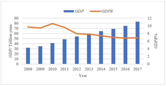
Figure 1.
Annual gross domestic product and growth rate in China from 2008 to 2017 * (* GDP (Gross domestic product), GDPR (GDP growth rate)).
The factors influencing the development of the freight industry in China are typically divided into two categories, namely, in- and out-systems. Out-system factors are related to national policies and regulations, such as trade policies and major national political decisions. In-system factors exist within the freight system, and include the infrastructure, resource inputs, and transportation outputs. To facilitate our research, this study analysed in-system factors. Infrastructure, resource inputs, and transportation outputs can be taken to comprehensively and objectively reflect the development of the freight industry. Therefore, this study makes use of these three in-system elements to evaluate the development of this industry.
3.1.2. Freight Index
Infrastructure, resource inputs, and transportation outputs include a variety of freight indices. First, this study determined a candidate index system based on these three aspects. Table 2 presents the specific candidate indices. As shown in Figure 2, the indices were selected one-by-one from the candidate indices.
Table 2.
Candidate freight indices.
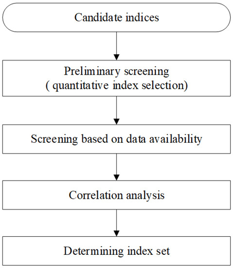
Figure 2.
Index selection procedure.
The first step was a preliminary selection based on the principle of quantitative analysis. The second step considered the availability of data collection, while the third step involved detecting index correlations. As freight turnover is the product of freight volume and transportation distance, this gives a full overview of freight transportation. This study took freight turnover as the benchmark index and used SPSS 21.0 software (IBM Corp. Released 2012. IBM SPSS Statistics for Windows, Version 21.0. Armonk, NY: IBM Corp) to analyse the correlations with indices [27]. In the fourth step, based on the results of the third step, the indices involved were adjusted as follows:
- (1)
- The total lengths of the railway mail line and employees of water transport industries with correlation coefficients of less than 0.2 were eliminated—three railway indices, including railway-freight volume, freight turnover, and transport employees had relatively low correlation coefficients. However, to reflect the importance of railway transport to the freight industry, these three indices were retained.
- (2)
- To ensure the independence and comprehensiveness of the index system, verifying the correlations of indices with similar meanings was necessary before the screening. The results showed that the correlation coefficient between the highway mileage and road network density was 0.916; between the railway operating mileage and railway network density was 1.0; between the inland waterway navigation mileage and waterway network density was 0.994, and; between the GDP and per capita GDP was 1.0. The highway mileage, railway operating mileage, inland waterway navigation mileage, and per capita GDP were retained based on the representativeness and recognition of each category of index. The correlation coefficient for the added value of the secondary industry and that of the construction industry was 0.993, where the latter was included in the former. The added value of the second industry was strongly representative so that the added value of the construction industry could be eliminated.
From the selection process of these indices, the freight indices of varied transportation modes were obtained. Table 3 shows the results. The letters in brackets represent the corresponding freight indices.
Table 3.
Freight index selection results.
3.2. Method
3.2.1. Standard Statistical Analysis
- (1)
- Stationarity Test
Whether a long-term relationship exists among variables (e.g., co-integration) depends on the stability of the variables. Therefore, it is essential that the data generation process for variables is stable before testing the co-integration and Granger causality.
The augmented Dickey–Fuller (ADF) test [28] is generally used to detect the stationarity of variables. However, the ADF test has a small sample. This problem can be dealt with by using the Dickey–Fuller generalised least square (DF-GLS) test [29], as was adopted in this study.
- (2)
- Co-Integration Test
The Co-integration of variables represents a stable long-term relationship. If two or more variables are non-stationary and have the same order of integration, they are said to be co-integrated. Where co-integration relationships exist, this study examines the coordination of varied freight modes.
The E-G co-integration test [30] is suitable for residual ADF testing, based on the co-integration regression estimation. The alternative hypothesis of co-integration among variables is used to test the null hypothesis without co-integration. Freight modes can have many indices; thus, this study uses the E-G two-step co-integration test and adopts F statistics within it.
- (3)
- Granger Causality Test
When information is complete, the lag value of the economic variable X can make economic variable Y more predictable; in this case, variable X is regarded as the Granger causality of variable Y. Granger causality is used when priority and predictability are under discussion.
To observe whether X affects Y depends on the extent to which the current Y can be explained by the past X. If X is helpful in predicting Y, or the correlation coefficient joining X and Y is statistically significant, the relationship between X and Y can be said to be of Granger causality.
3.2.2. Spatial Autocorrelation Test
Spatial econometrics deals with spatial dependence and spatial heterogeneity, which are not only critical aspects of data used by regional scientists, but also important methods for use in the freight industry and the regional economic research conducted by transport scholars.
The spatial autocorrelation test, which includes global and local spatial autocorrelation analyses, is a common method of studying regional differences. This study adopted both global and local spatial autocorrelation tests to examine the spatial autocorrelation distributions of the coordination between varied freight modes and the economies of varied regions.
Global spatial autocorrelation tests whether a region displays agglomeration, particularly by estimating the locations of agglomeration regions, as the results are reliable. Global autocorrelation is used to detect the spatial effect of an entire research area and to cover up the spatial relationships among adjacent areas. Moran’s I is an important index for evaluating spatial correlation. This study uses Moran’s I [31] to reflect the global spatial autocorrelation between freight transport and the economy. This coefficient is calculated based on the following formula:
where refers to the number of spatial units; refers to the observed value; refers to the mean value of ; and refers to the spatial connection matrix between spatial units and .
The value range of Moran’s I is (−1,1). A value of over 0 represents a positive correlation, and a value of less than 0 represents a negative. In addition, a larger absolute value indicates a larger spatial autocorrelation among regions, and vice versa. When the value is close to 0, space presents a random distribution.
Through local spatial autocorrelation analysis, the spatial aggregation points in the study area can be determined, and the local spatial autocorrelation reflects the degree of correlation between the study area and its adjacent areas. Local indices of spatial association (LISA) were proposed by Anselin [32]. These indices can decompose Moran’s I coefficient, analysed by way of local spatial autocorrelation into the local spaces. This study uses LISA as the index of local spatial autocorrelation analysis. The formula for calculating this is:
where
4. Coordination Model
The integration of freight indices and the economy can be used to reflect the relationship between the economy and freight transport. We first examined the causal links between freight indices and the economy, and then on this basis, analysed the coordination of single and varied freight modes. At the same time, based on the coordination model for varied-freight modes, the economy, and spatial autocorrelation tests, we analysed the regional spatial autocorrelation characteristics of the coordination among varied freight modes and the economy.
On the basis of the differences in regional development in China, the country was divided into four regions—the Eastern, Western, Northeast, and Central regions to investigate the relationship between freight transport and the economies of varied regions. The Eastern region included Hainan, Guangdong, Fujian, Zhejiang, Jiangsu, Shanghai, Shandong, Hebei, Beijing, and Tianjin, a total of 10 provinces and cities; the Central region included Hubei, Hunan, Henan, Anhui, Jiangxi, and Shanxi, a total of six provinces; the Western region included Guangxi, Yunnan, Guizhou, Sichuan, Chongqing, the Tibet Autonomous Region, Qinghai, Shaanxi, Gansu, the Ningxia Hui Autonomous Region, the Xinjiang Uygur Autonomous Region, and the Inner Mongolia Autonomous Region, a total of 12 provinces and cities; and the Northeast region included Liaoning, Jilin, and Heilongjiang, a total of three provinces.
4.1. Coordination Model for Single-Freight Mode
We call the internal coordination model of single-mode of freight transportation the for short. It is based on the DEA model. This study takes the coordination of road freight as an example. The process of establishing the model is as follows:
- (1)
- The decision-making unit is one year. Coordination within the highway transportation system is analysed yearly, and input and output indices are constructed—four of the former and two of the latter. Each mode of transportation is different from the others. Table 4 shows the input and output indices for each.
Table 4. Input and output indices of varied modes of transportation.
- (2)
- The input index vector for the highway transportation mode is set as , where refers to the value of the m input index of a certain transportation mode in year i; the output index vector of each transportation mode is , where refers to the value of the n output index of a certain transportation mode in year i.
- (3)
- The efficiency of a certain transportation mode is calculated for year i, on the basis of the following formula:where signifies the efficiency in year and , while and are the weights of the output and input indices.
- (4)
- The coordination model is constructed for year i on the basis of Equation (4):where and signify the weights of the output and input indices, respectively. The meanings of the other parameters are the same as those in the previous formula.
For convenience, this model was transformed into a linear programming model. Here,
The formula after transformation is:
The meanings of the parameters are the same as those in Equations (4) and (5). Equation (7) gives the mathematical model for coordination in the highway-freight mode. The construction method for the coordination models of the other three freight modes can be obtained by referring to the coordination model for the highway-freight mode.
4.2. Coordination Model for the Varied-Freight Mode
We call the coordination model among the varied modes of freight transport the varied-freight model for short. This can be improved and obtained based on the DEA basic model [33,34]. Based on the DEA model, the Charnes, Cooper, and Rhodes (CCR) model has been adopted. This model improves the original DEA by generalizing the single-output to single-input classical engineering ratio definition to multiple inputs and outputs. Assuming that a and b are two transportation modes, the input of transportation mode a is used as the input index of the model, while the output of transportation mode b is regarded as the output index. Then, the coordination of a and b can be modelled according to this principle. The improved linear programming mathematical model is
where represents the coordination of two transportation modes, ; refers to the ith output variable, ; refers to the ith output variable, ; refers to the weight of the input parameters; and refers to the weight of the output parameters.
The dual-programming model is obtained by introducing the slack variable as:
where refers to the unknown variable and slack variable , and m and n refer to the amounts of the input and output indices, respectively. refers to the coordination of transportation mode a with transportation mode b, but not vice versa.
or reflects how one transportation mode is coordinated with another, but cannot represent the nature of this coordination [35]. This study reflects the coordination of varied transportation modes on the basis of the static coordination between them. The formula for calculating the coordination is
Equation (10) can be used to calculate the coordination among different freight modes. Generally, the value of coordination lies between 0 and 1, with 1 representing a fully coordinated state of transportation, and 0 the opposite. Table 5 shows the coordination classifications of the two freight modes [36].
Table 5.
Coordination classification criteria.
For the procedure of calculation for the coordination degree among pairs of freight modes, see Figure 3.
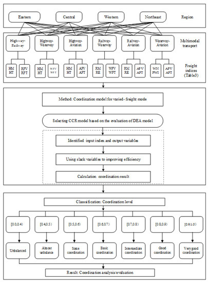
Figure 3.
Calculating procedure for coordination degree among pairs of freight modes *. * Data Envelopment Analysis (DEA).
The four steps of coordination calculation and evaluation among pairs of freight modes are as follows:
Step 1: Regional division. As mentioned above, China is divided into four regions, according to their economic and geographical characteristics, as well as the development of regional planning.
Step 2: Transport mode division. There are six types of multi-transport modes in pairs, including the highway-railway, highway-waterway, highway-aviation, railway-waterway, railway-aviation, and waterway-aviation. The specific input and output variables are shown in Table 6.
Table 6.
Input and output variables of various multi-transport modes.
Step 3: Coordination calculation. A CCR model is selected to calculate input and output index values by using DEAP software, and the coordination value is calculated by introducing the slack variable.
Step 4: Coordination analysis and evaluation. The coordination level is determined for multi-transport in pairs, such as highway-railway, according to Table 5.
4.3. Coordination Model among Varied-Freight Modes and the Economy
From the history of the mutual influence and common development of freight transport and the economy, when freight meets the needs of economic development, it plays an important role in promoting the development of the economy. When it lags behind the development of the economy, it delays the development of the latter, and when rapid development of the economy leads to a large requirement for transportation, this development will have an effect on the freight industry, accelerating its reform and development, and driving it to keep up with social and economic growth. A relationship exists between freight transport and the economy, and therefore, the coordination model of varied freight modes and the economy can be determined by the efficacy function connecting them.
4.3.1. Efficacy Function
On the basis of the principle of multiple-objective programming, the evaluation index sample of the evaluation object is standardised by referring to the measurement standard, and is transformed into a comparable efficacy function.
To set the variable as an order parameter of the freight-economic system, its value is , which includes the annual transportation infrastructure index, resource input index, transportation output index, and GDP index. , were used to calculate the upper and lower limit values corresponding to the respective regions.
The efficacy of the order parameter of freight and the economy on the system order can be expressed as:
where refers to the efficacy of the variable , such as the infrastructure index, resource input index, transportation output index, and GDP on the system order, and A refers to the stable region of the system.
4.3.2. Coordination Function
The coordination function includes two categories: the linear-weighting and geometric-average methods. The linear-weighting method must determine the weight coefficient with a certain level of subjectivity; therefore, this study adopts the geometric-average method to calculate the coordination function as:
where C is the coordination value, and the other variables are used in the same manner as seen above.
5. Results and Discussion
Based on the freight volumes of varied freight modes and the development data for China from 2008 to 2017, the causality test was first carried out for the selected freight indices and the economy.
5.1. Causality Test for Freight Indices and the Economy
This study first tested the stationarity of variables. On this basis, the co-integration and Granger causality of the freight indices and economic growth were tested.
5.1.1. Stationarity Test Results
This study used Eviews 9.0 (Eviews Version 9.0, HIS Global Inc. Irvine, CA, USA) software to undertake a stationarity test for the GDPR. Table 7 shows the test results, where DGDPR refers to the first-order difference of GDPR.
Table 7.
Dickey–Fuller generalised least square (DF-GLS) test results.
In Table 7, the variable GDPR clearly passes the stationarity test at a 1% significance level after the first-order difference. This indicates that the GDPR is an integrated time-series with a 1% significance level.
5.1.2. Co-Integration Test Results
In the E-G two-step method, the ordinary least-squares method (OLS) was first adopted to construct the GDPR regression equations with WNP, HFV, HFT, and WFV (see Equation (13)), which is a method assuming that the analysis fits a model of a relationship between one or more explanatory variables and a continuous, or at least interval outcome variable that minimizes the sum of square errors. To reduce errors, a dimensionless treatment of the data shall be conducted before the construction of the equation:
where GDPR refers to economic growth rate; WNP refers to the net load of a power-driven boat; HFV refers to highway-freight volume; HFT refers to highway-freight turnover; WFV refers to waterway-freight volume; and refer to the residuals of corresponding variables.
The residuals were saved, and those of WNP, HFV, HFT, and WFV were tested using DF-GLS. Table 8 shows that the four indicators passed the test at a 5% significance level, which means that WNP, HFV, HFT, and WFV have a long-term, stable, co-integration relationship with GDPR.
Table 8.
Regression equation residual test results.
5.1.3. Granger Causality Results
Granger causality is a method of measuring the interactions among variables in a time series. This study carried out a Granger causality test for GDPR and 19 freight indices based on the AIC and SC minimum criteria. The hypothesis given in Table 8 was adopted in the test. A vector autoregression model (VAR) was used to determine the optimal lag periods of two variables to be 1, and Appendix A shows the Granger causality test results. In Appendix A, HT WNP, HFV, HFT, and WFV are shown to be unidirectional Granger causes of GDPR, while the GDPR is a unidirectional Granger cause of HT, and Table 9 shows the causality test results.
Table 9.
Freight indices and the GDPR * causality test.
Single co-integration of the same order is a precondition for the Granger causality test, in which the HT and HE do not meet. Therefore, the DF-GLS test for WNP, HFV, HFT, and WFV was conducted, with test results shown in Table 10.
Table 10.
The DF-GLS test results.
In Table 10, WNP, HFV, HFT, and WFV show the same first-order single co-integration as GDPR at a 1% significance level. At the same time, based on the test results shown in Appendix A, the waterway net load of power-driven boats (WNP), highway freight volume (HFV), highway freight turnover (HFT), and waterway freight volume (WFV) are the Granger causes of the national economic growth rate or GDPR.
These test results reflect the co-integration of freight indices and social relations. On this basis, this study examined and analysed the coordination of regional single and varied freight modes and the spatial autocorrelation of the coordination between varied freight modes and the economy.
5.2. Analysis of the Coordination of the Regional Single-Freight Mode
This study adopted Equation (7) for the single-freight mode coordination model. In this model, Table 4 presents the input and output indices of each freight model, based on which the degree of coordination of the single-freight mode in different regions was calculated. Table 11 presents the results of the calculations.
Table 11.
Coordination among four freight modes in different regions.
Based on the classification criteria in Table 5, Table 11 shows that the coordination among the four freight modes in different regions is good or high-quality.
The highway-freight mode is strong in the four regions. This indicates that this mode has good coordination throughout China, and shows its strong prospects for development. The railway-freight mode also has good coordination throughout the regions, which may be related to the government’s emphasis on this form of transportation. The waterway and aviation freight modes are also well-coordinated in every region, which is possibly due to the rapid development of the express logistics industry in recent years.
5.3. Analysis of the Coordination between Freight Modes in Different Regions
Based on the coordination model of varied freight modes established in Equations (8)–(10), the degrees of coordination of varied freight modes in the Eastern, Central, Western, and Northeast regions are calculated.
Table 12 shows the results of the calculations. Here, H refers to the highway-freight mode; R refers to the railway-freight mode; W refers to the waterway-freight mode; and A refers to the aviation-freight mode. Table 12 also shows that the highway-railway freight modes were in a good state, C(H,R) = 0.892, 0.865, 0.873, in the Eastern, Central, and Western regions, and an intermediate state, C(H,R) = 0.751, in the Northeast region. The highway-waterway freight modes exhibited very good coordination in the Eastern and Northeast regions, good coordination in the Western region, and basic coordination in the Central region. The highway-aviation freight modes had very good coordination in the Eastern, Western, and Northeast regions, while in the Central region, their coordination was intermediate. However, the railway-waterway freight modes had intermediate coordination in the Eastern, Western, and Northeast regions, but were rarely coordinated in the Central region. The railway-aviation freight modes had very good coordination in the Eastern and Western regions, and intermediate coordination in the other two regions. Meanwhile, the waterway-aviation freight modes had very good coordination in the Northeast, and good coordination in the other three regions.
Table 12.
Coordination among pairs of freight modes in different regions.
The coordination results were analysed and evaluated using DEAP 2.1 software (see Table 12). The coordination degree for highway and railway multi-transport transport in the eastern region was found to be 0.892, which is considered good coordination, as shown in Table 5. Amid increasing economic development in eastern China, investments in highway construction have been further expanded. The total mileage of highways in operation has risen from 949,100 km in 2008 to 1,151,200 km in 2017, with an average annual growth of 2.3%. The number of trucks in use on China’s highways increased from 3.151 million in 2008 to 5.257 million in 2017, an average annual increase of 5.8%. In turn, this promoted the average annual growth of railway freight volume and turnover volume by 0.6% and 1.3%, respectively, with good coordination seen between the highways and railways.
From Table 12 in the Central region, it can be seen that the highway-railway freight modes and waterway-aviation freight modes have good coordination, but that there is huge room for improvement in the coordination of the other freight modes. The latter should be strengthened in this region to promote economic development. This finding also verifies the viewpoint of Yu et al. [37]. Taking into account all four regions of China, developing good coordination of land (road and rail) transport modes is consistent with the conclusions of Hong et al. [38]. However, the coordination of aviation transport with the other modes contradicts this viewpoint.
5.4. Spatial-Autocorrelation Analysis of the Coordination of the Varied-Freight Model
5.4.1. Global Spatial Autocorrelation
The coordination between varied freight modes (highway, rail, water, and aviation) and economic development can be calculated using Equations (11) and (12). The coordination results for the Eastern, Central, Western, and Northeast regions in 2010, 2012, 2015, and 2017 are shown in Table 13.
Table 13.
Coordination of the four different regions in different years.
Figure 4 shows the changes in the coordination of the four regions in those four years. This suggests that, in those years, the coordination among freight modes and the economies of China’s four regions slowly rose.
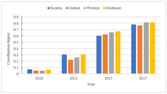
Figure 4.
Changes in the coordination of the four regions in different years.
The coordination among the freight modes and the economies in 2010 and 2012 was poor and unbalanced, possibly due to the world financial crisis of 2008. In 2015 and especially 2017, the coordination improved, possibly due to the promotion via economic reform of the coordination among freight modes and economies.
According to the data in Table 13, Moran’s I was calculated based on Equation (1), and Table 14 shows the results of this calculation. At the same time, the changes in Moran’s I of the four regions in different years were obtained, as shown in Figure 5.
Table 14.
Moran’s I for the four regions in different years.
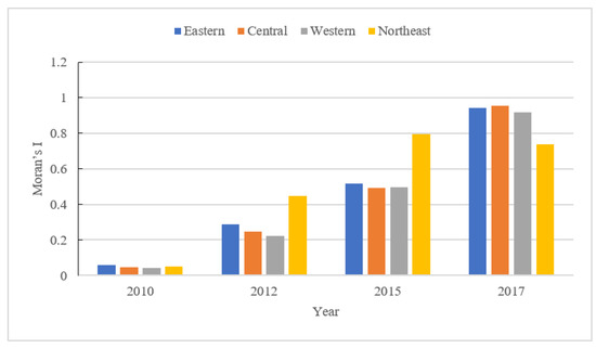
Figure 5.
Changes in Moran’s I for the four regions in different years.
From Figure 5, we find that Moran’s I, representing the coordination between freight transport and the economies of the four regions in 2010, were relatively low and stable over time, while in 2012 and 2014 they rose in every region. The growth rates in the Northeast region in 2012 and 2014 were 83.3% and 61.1%, respectively, of those of the Central region. The spatial correlation also increased. The indices in the Eastern, Central, and Western regions in 2017 increased over their 2014 levels, while the indices in the Northeast region fell by 7.3%.
The Moran’s I results show that the coordination between freight transport and the economy of the Eastern region was relatively small in 2010, but then slowly increased. The spatial correlation of the coordination in the Eastern region grew from weak to strong, with enhanced aggregation.
Changes in Moran’s I representing the coordination in the Central and Western regions in different years were similar to those in the Eastern region. The coordination between freight transport and the economies of the Central and Western regions increased accordingly, a finding that is consistent with the viewpoint of Fan et al. [39]. However, in the Northeast, Moran’s I increased in 2010, 2012, and 2014, then fell in 2017. The spatial correlation between freight transport and the economy of the Northeast in the first three years slowly intensified, with aggregation increasing accordingly. In 2017, the spatial correlation and aggregation became weaker.
5.4.2. Local Spatial Autocorrelation
Based on the calculation results, we drew Moran scatter plots of the four regions in different years. The quadrant of each point in the scatter plot reflects the spatial-autocorrelation distribution and correlation of the coordination between the freight transport and economy of each region. Figure 6 shows the Moran scatter plots.
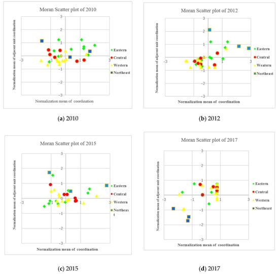
Figure 6.
Moran scatter plots of the coordination in the four regions in different years.
From Figure 6, we find that the Northeast was in the high-high quadrant in 2012 and 2015, but fell to the low-low quadrant in 2017. This indicates that the coordination between freight transport and the economy in the Northeast fell after 2015. However, the Central and Western regions were in the low-low quadrant in 2012 and 2015 and jumped to the high-high quadrant in 2017, indicating that freight transport in these regions had made progress.
A spatial LISA cluster graph can be obtained through spatial clustering based on the calculation of the LISA index. The LISA cluster graph can be used to show the correlation of the coordination of all regions in space. To further test the spatial dependence of the coordination, ArcGIS software was used to draw the LISA aggregation diagrams of the four regions in different years, on the basis of calculating the LISA values for each region, as shown in Figure 7.
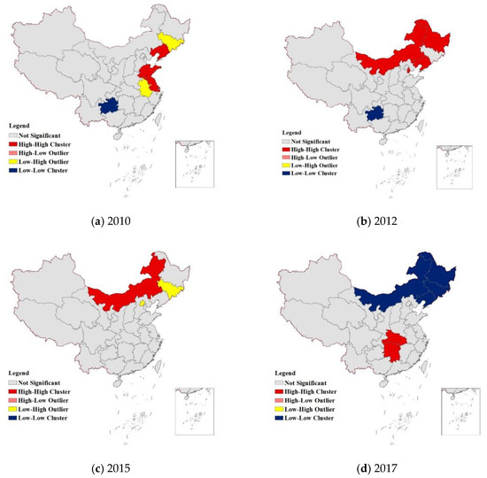
Figure 7.
Local indices of spatial association (LISA) aggregation diagrams for the four regions in different years.
In the LISA aggregation diagrams, different colours represent varied types of aggregation. The red area (high–high) shows that the coordination of a sub-region and its adjacent sub-region was relatively strong, while the blue area (low-low) shows that this coordination was relatively weak. The yellow area (low-high) shows that the coordination of a sub-region was relatively weak, while the coordination of its adjacent sub-region was relatively strong, and the pink area (high-low) shows that the coordination of a region was relatively strong, while the coordination of its adjacent sub-region was relatively weak. The grey area shows that the autocorrelation of the coordination of a sub-region is insignificant; it is called an insignificant area.
Figure 7 shows the location of the agglomeration mode and its corresponding changes in four regions of China in different years. See Table 15 for the changes in agglomeration mode in different years.
Table 15.
Aggregation modes of the four regions in different years.
5.4.3. Discussion
Table 15 shows that the high–high and insignificant aggregation modes appeared in the Eastern region in 2010, and gradually became insignificant in the other three periods, which shows that the spatial autocorrelation of the coordination between freight and economy in the Eastern region is not obvious in the four periods, and its correlation has great room for improvement; however, this is contrary to the opinion of Yu et al. [19]. Moreover, the correlation in the Central region was insignificant in 2012 and 2015, but insignificant and low–high, and insignificant and high–high in 2010 and 2017, respectively. Thus, significant differences can be found over time in the spatial correlation of the Central region. Therefore, giving full play to the pivotal role of various modes of transportation in the Central region is essential to promoting economic development there.
For the four different years above, there were numerous agglomeration modes seen in the western and northeastern regions of China, among which the spatial correlation of the whole western region shows no significant mode, while the local region shows a positive correlation mode. For example, the mode was high–high for Inner Mongolia in 2012 and 2015, but low–low in 2017. This may be related to Inner Mongolia maximising its potential for tourism by constructing transportation infrastructure in recent years. The mode was low–low in Guizhou in 2010 and 2012, which is related to Guizhou’s investment in transportation infrastructure. In the Northeast, the modes for Heilongjiang were insignificant, high–high, and insignificant for 2010, 2012, and 2015, respectively, while for Jilin they were low–high, insignificant, and low–high, and for Liaoning, high–high and insignificant. In 2017, a low–low positive-correlation mode prevailed in the three northeastern provinces. Large differences existed in the spatial correlations among various freight modes and the economy of the Northeast, and the coordinated development of various freight modes and the economies of different regions were relatively poor. This may have been caused by the lack of vitality of economic development in the Northeast, weak transport infrastructure, and a low density of road networks.
6. Conclusions
The causality test was first carried out for the freight and socio-economic indices, after which this study established the coordination models for single and varied-freight modes. Moreover, the spatial correlation of the coordination between the varied freight modes and the economy was analysed on the basis of these modes, the economic-coordination model, and the spatial-autocorrelation test. Finally, China’s 2008–2017 data for the varied modes of freight transport and the economy was collected and used as a basis for analysis. The following are the conclusions of this research.
- (1)
- We selected 19 freight indices and conducted co-integration and Granger causality analysis for these and socio-economic GDPR. The results showed that the net loads of power-driven boats, highway-freight volumes, highway-freight turnover, and waterway-freight volumes had a long-term co-integration relation with GDPR.
- (2)
- A coordination model for the single freight mode was established. Based on the 19 freight indices, the coordination of varied freight modes across the country was analysed, and throughout the regions, the coordination was good, at over 0.80.
- (3)
- A coordination model for the varied freight modes was established, and waterway and aviation freight were shown to be well-coordinated in the four regions, with coordination exceeding 0.83. The coordination between railway and waterway freight in the Eastern region was 0.78; however, the coordination of the other freight modes exceeded 0.90.
- (4)
- Based on the coordination model for varied freight modes, the economy, and the spatial-autocorrelation test, the global and local spatial autocorrelations of the coordination of varied freight modes and economies were analysed. The results showed that the spatial correlation between the varied modes of transportation and the economies in the Eastern and Western regions was insignificant as a whole, and the regional differences in the spatial correlation between varied modes of transportation and the economies of the Central and Northeast regions were obvious.
As one of the indicators of transportation output, freight revenue plays an important role. At present, the statistics based on freight revenue data for China are relatively limited. Railway freight revenue data were only available for the years 2008–2017, while a freight revenue system for civil aviation was not established until 2015. Other modes of transportation, including highway and waterway transportation, also suffer from a lack of relevant freight revenue statistics. However, the paper indirectly considers economic indicators, such as the added value of the first, second, and tertiary industries for analysing the relationship between freight and the economy, which to some extent makes up for the impact of freight revenue indicators. In the future, with the gradual improvement of China’s statistical system and the application of emerging technologies in the areas of big data and cloud computing, freight revenues for various modes of transportation will be incorporated into the statistical system. Furthermore, the quality of freight revenue data will be further improved, and subsequent comprehensive freight index research will be taken into consideration.
In addition, restricted by the data analysis methods and models, this study only analysed the coordination between the highway and railway freight transportation systems for different regions and provinces in China; how the overall coordination among three or even four modes of freight transportation can be measured is one of the directions for future research. The verification of the interactions between freight transport and the social economy is mainly based on the national data level, and the impact of freight systems on different regions on the social economy was not considered. Further research can be carried out for the specific parameters of the coordination model. In addition, the impact of various indicators on the coordination between freight transport and the economy in different regions also requires more detailed analysis.
Author Contributions
The authors confirm contribution to the paper as follows: conceptualization, Y.Z. and Y.G.; data curation, Y.G.; formal analysis, Y.G., X.Z. and Y.M.; funding acquisition, Y.G. and Y.Z.; methodology, Y.G.; project administration, Y.G and Y.Z.; resources, Y.G., C.L. and X.Z.; validation, Y.Z., X.Z. and R.C.; writing—original draft, Y.G.; writing—review and editing, Y.G., Y.Z., X.Z., R.C., Y.M., and C.L. All authors have read and agreed to the published version of the manuscript.
Funding
This research received no external funding.
Acknowledgments
The authors acknowledge the anonymous reviewers for their valuable comments and suggestions. This work was supported by the project of the National Development and Reform Commission of the People’s Republic of China, “Research on the Relationship between the Adjustment of Transportation Structure and the Quality and Efficiency of Economic Operation (2018–2019)”.
Conflicts of Interest
The authors declare no conflict of interest.
Appendix A
Table A1.
Results of the Granger causality test.
Table A1.
Results of the Granger causality test.
| Null Hypothesis | Observed Value | F Statistics | p-Value | Conclusions |
|---|---|---|---|---|
| HM cannot cause GDPR variation | 8 | 5.2212 | 0.1054 | Accept |
| GDPR cannot cause HM variation | 8 | 2.4498 | 0.234 | Accept |
| HT cannot cause GDPR variation | 8 | 19.434 | 0.0192 | Reject |
| GDPR cannot cause HT variation | 8 | 0.3520 | 0.7289 | Accept |
| RM cannot cause GDPR variation | 8 | 1.0405 | 0.4537 | Accept |
| GDPR cannot cause RM variation | 8 | 1.3065 | 0.3907 | Accept |
| WM cannot cause GDPR variation | 8 | 6.8016 | 0.0768 | Accept |
| GDPR cannot cause WM variation | 8 | 0.7303 | 0.5516 | Accept |
| WNP cannot cause GDPR variation | 8 | 59.516 | 0.0039 | Reject |
| GDPR cannot cause WNP variation | 8 | 0.4831 | 0.6579 | Accept |
| AN cannot cause GDPR variation | 8 | 1.4602 | 0.3607 | Accept |
| GDPR cannot cause AN variation | 8 | 4.5396 | 0.1238 | Accept |
| HI cannot cause GDPR variation | 8 | 8.2100 | 0.0607 | Accept |
| GDPR cannot cause HI variation | 8 | 1.3646 | 0.3789 | Accept |
| HE cannot cause GDPR variation | 8 | 4.3427 | 0.1301 | Accept |
| GDPR cannot cause HE variation | 8 | 38.544 | 0.0072 | Reject |
| RE cannot cause GDPR variation | 8 | 1.8641 | 0.2977 | Accept |
| GDPR cannot cause RE variation | 8 | 3.717 | 0.1542 | Accept |
| WI cannot cause GDPR variation | 8 | 2.6872 | 0.2144 | Accept |
| GDPR cannot cause WI variation | 8 | 0.0581 | 0.9446 | Accept |
| AE cannot cause GDPR variation | 8 | 6.3858 | 0.083 | Accept |
| GDPR cannot cause AE variation | 8 | 0.373 | 0.7167 | Accept |
| HFV cannot cause GDPR variation | 8 | 13.789 | 0.0307 | Reject |
| GDPR cannot cause HFV variation | 8 | 0.1854 | 0.8396 | Accept |
| HFT cannot cause GDPR variation | 8 | 10.02 | 0.047 | Reject |
| GDPR cannot cause HFT variation | 8 | 0.2956 | 0.7635 | Accept |
| RFV cannot cause GDPR variation | 8 | 1.3085 | 0.3903 | Accept |
| GDPR cannot cause RFV variation | 8 | 0.1634 | 0.8564 | Accept |
| RFT cannot cause GDPR variation | 8 | 1.0054 | 0.4633 | Accept |
| GDPR cannot cause RFT variation | 8 | 0.716 | 0.5569 | Accept |
| WFV cannot cause GDPR variation | 8 | 31.8916 | 0.0095 | Reject |
| GDPR cannot cause WFV variation | 8 | 0.9655 | 0.4745 | Accept |
| WFT cannot cause GDPR variation | 8 | 9.3022 | 0.0517 | Accept |
| GDPR cannot cause WFT variation | 8 | 1.2677 | 0.399 | Accept |
| AFV cannot cause GDPR variation | 8 | 4.6897 | 0.1193 | Accept |
| GDPR cannot cause AFV variation | 8 | 4.4958 | 0.1251 | Accept |
| AFT cannot cause GDPR variation | 8 | 0.5355 | 0.6326 | Accept |
| GDPR cannot cause AFT variation | 8 | 1.2172 | 0.4102 | Accept |
References
- Easterly, W.; Rebelo, S. Fiscal policy and economic growth. J. Monet. Econ. 1993, 32, 417–458. [Google Scholar] [CrossRef]
- Cain, L.P. Historical perspective on infrastructure and US economic development. Reg. Sci. Urban Econ. 1997, 27, 117–138. [Google Scholar] [CrossRef]
- Chi, J.; Baek, J. Dynamic relationship between air transport demand and economic growth in the United States: A new look. Transp. Policy 2013, 29, 257–260. [Google Scholar] [CrossRef]
- Kiyohito, U. Social capital and local public transportation in Japan. Res. Transp. Econ. 2016, 59, 434–440. [Google Scholar]
- Boopen, S. Transport infrastructure and economic growth: Evidence from Africa using dynamic panel estimates. Empir. Econ. Lett. 2006, 5, 37–52. [Google Scholar]
- Herranz-Loncán, A. Infrastructure investment and Spanish economic growth, 1850–1935. Explor. Econ. Hist. 2007, 44, 452–468. [Google Scholar] [CrossRef]
- Zahra, A.; Razzaq, S.; Nazir, A. Impact of Electricity Consumption and Transport Infrastructure on the Economic Growth of Pakistan. Int. J. Acad. Res. Bus. Soc. Sci. 2016, 6, 291–300. [Google Scholar] [CrossRef]
- Pradhan, R.P. Transport Infrastructure, Energy Consumption and Economic Growth Triangle in India: Cointegration and Causality Analysis. J. Sustain. Dev. 2010, 3, 167–173. [Google Scholar] [CrossRef]
- Pradhan, R.P. Modelling the nexus between transport infrastructure and economic growth in India. Int. J. Manag. Decis. Mak. 2010, 11, 182–196. [Google Scholar] [CrossRef]
- Pradhan, R.P.; Bagchi, T.P. Effect of transportation infrastructure on economic growth in India: The VECM approach. Res. Transp. Econ. 2013, 38, 139–148. [Google Scholar] [CrossRef]
- Brida, J.G.; Rodriguez-Brindis, M.A.; Lanzilotta, B.; Rodriguez-Collazo, S. Testing linearity in the long-run relationship between economic growth and passenger air transport in Mexico. Int. J. Transp. Econ. 2016, 43, 437–450. [Google Scholar]
- Keho, Y.; Echui, A.D. Transport Infrastructure Investment and Sustainable Economic Growth in Côte d’Ivoire: A Cointegration and Causality Analysis. J. Sustain. Dev. 2011, 4, 23–35. [Google Scholar] [CrossRef]
- Marazzo, M.; Scherre, R.; Fernandes, E. Air transport demand and economic growth in Brazil: A time series analysis. Transp. Res. Part E: Log. Transp. Rev. 2010, 46, 261–269. [Google Scholar] [CrossRef]
- Maparu, T.S.; Mazumder, T.N. Transport infrastructure, economic development and urbanization in India (1990–2011): Is there any causal relationship. Transp. Res. Part A Policy Pract. 2017, 100, 319–336. [Google Scholar] [CrossRef]
- Beyzatlar, M.A.; Karacal, M.; Yetkiner, H. Granger-causality between transportation and GDP: A panel data approach. Transp. Res. Part A Policy Pract. 2014, 63, 43–55. [Google Scholar] [CrossRef]
- Njoku, C.O.; Chigbu, E.E.; Akujuobi, A.B.C. Public Expenditure and Economic Growth in Nigeria: A Granger Causality Approach 1983–2012. Manag. Stud. Econ. Syst. 2015, 1, 147–160. [Google Scholar] [CrossRef][Green Version]
- Saidi, S.; Hammami, S. Modeling the causal linkages between transport, economic growth and environmental degradation for 75 countries. Transp. Res. D Transp. Environ. 2017, 53, 415–427. [Google Scholar] [CrossRef]
- Yu, N.; de Jong, M.; Storm, S.; Mi, J. Transport Infrastructure, Spatial Clusters and Regional Economic Growth in China. Transp. Rev. 2011, 32, 3–28. [Google Scholar] [CrossRef]
- Kustepeli, Y.; Gulcan, Y.; Akgungor, S. Transportation infrastructure investment, growth and international trade in Turkey. Appl. Econ. 2012, 44, 2619–2629. [Google Scholar] [CrossRef]
- Bhunia, A. An empirical study between government sectoral expenditure and Indian economic growth. Econ. Bull. 2011, 31, 1–47. [Google Scholar]
- Shin, S.; Roh, H.; Hur, H.S. Characteristics Analysis of Freight Mode Choice Model According to the Introduction of a New Freight Transportation System. Sustainability 2019, 11, 1209. Available online: https://www.mdpi.com/2071-1050/11/4/1209 (accessed on 21 February 2020). [CrossRef]
- Zhao, J.; Zhu, X.; Wang, L. Study on Scheme of Outbound Railway Container Organization in Rail-Water Intermodal Transportation. Sustainability 2020, 12, 1519. Available online: https://www.mdpi.com/2071-1050/12/4/1519 (accessed on 21 February 2020).
- Boarnet, M.G. Spillovers and Locational Effects of Public Infrastructure. J. Reg. Sci. 1998, 38, 381–400. [Google Scholar] [CrossRef]
- Gillen, D.W. Transportation infrastructure and economic development: A review of recent literature. Logist. Transp. Rev. 1996, 32, 39–62. [Google Scholar]
- Bougheas, S.; Demetriades, P.O.; Mamuneas, T.P. Infrastructure, specialization, and economic growth. Can. J. Econ. 2000, 33, 506–522. [Google Scholar] [CrossRef]
- National Bureau of Statistics of China. China Statistical Yearbook; China Statistics Press: Beijing, China, 2007–2018.
- Lahiri, K. Chapter 2 Composite Coincident Index of the Transportation Sector and Its Linkages to the Economy. In Transportation Indicators and Business Cycles; Emerald Group Publishing Limited: Bingley, UK, 2010; Volume 289, pp. 39–56. [Google Scholar]
- Dickey, D.A.; Fuller, W.A. Likelihood ratio statistics for autoregressive time series with a unit root. Econometrica 1981, 49, 1057–1072. [Google Scholar] [CrossRef]
- Elliott, G.; Rothenberg, T.J.; Stock, J.H. Efficient tests for an autoregressive unit root. Econometrica 1992, 64, 813–836. [Google Scholar] [CrossRef]
- Engle, R.F.; Granger, C.W.J. Co-integration and error correction: Representation, estimation, and testing. Econometrica 1987, 55, 251–276. [Google Scholar] [CrossRef]
- Xu, J. Geographical Modelling Methods; Science Press: Beijing, China, 2010. [Google Scholar]
- Anselin, L. Spatial Econometrics: Methods and Models; Kluwer Academic: Dordrecht, The Netherlands, 1988. [Google Scholar]
- Charnes, A.; Cooper, W.W.; Rhodes, E. Measuring the efficiency of decision making units. Eur. J. Oper. Res. 1978, 2, 429–444. [Google Scholar] [CrossRef]
- Charnes, A. Sensitivity analysis of the additive model in Data Envelopment Analysis. Eur. J. Oper. Res. 1990, 48, 332–341. [Google Scholar] [CrossRef]
- Fried, H.O.; Lovell, C.A.K.; Schmidt, S.S.; Yaisawarng, S. Accounting for Environmental Effects and Statistical Noise in Data Envelopment Analysis. J. Prod. Anal. 2002, 17, 157–174. [Google Scholar] [CrossRef]
- Luan, X.; Cheng, L.; Yu, W.; Zhou, J. Multimodal Coupling Coordination Analysis at the Comprehensive Transportation Level. J. Transp. Syst. Eng. Inf. Technol. 2019, 3, 27–33. [Google Scholar]
- Yu, N.; De Jong, M.; Storm, S.; Mi, J. The growth impact of transport infrastructure investment: A regional analysis for China (1978–2008). Policy Soc. 2012, 31, 25–38. [Google Scholar] [CrossRef]
- Hong, J.; Chu, Z.; Wang, Q. Transport infrastructure and regional economic growth: Evidence from China. Transportation 2011, 38, 737–752. [Google Scholar] [CrossRef]
- Fan, S.; Chan-Kang, C. Regional road development, rural and urban poverty: Evidence from China. Transp. Policy 2008, 15, 305–314. [Google Scholar] [CrossRef]
© 2020 by the authors. Licensee MDPI, Basel, Switzerland. This article is an open access article distributed under the terms and conditions of the Creative Commons Attribution (CC BY) license (http://creativecommons.org/licenses/by/4.0/).