Trajectory Data Analysis on the Spatial and Temporal Influence of Pedestrian Flow on Path Planning Decision

Abstract

The modeling of walking behavior and design of walk-friendly urban pathways have been of interest to many researchers over the past decades. One of the major issues in pedestrian modeling is path planning decision-making in a dynamic walking environment with different pedestrian flows. While previous studies have agreed that pedestrian flow influences path planning, only a few studies have dealt with the empirical data to show the relationship between pedestrian flow and path planning behavior. This study introduces a new methodology for analyzing pedestrian trajectory data to find the dynamic walking conditions that influence the path planning decision. The comparison of the pedestrians’ path shows that the higher proportion of opposite flows are, the greater they influence the path selection decision. In this study, we investigate the relationship between the opposite flow changes and path planning behavior and find the spatial and temporal ranges of the opposite flow that affects the path planning behavior. Lastly, we find the ratio of pedestrians that update their paths with respect to the opposite flow rate.

1. Introduction

Walking is one of the main modes used for short trips, and it can also serve as a connection to other modes in multimodal trips. As the urban area increases and the level of transportation services are degraded, transportation planners have encouraged travelers to walk more by designing a safe and convenient walking environment. Accordingly, the understanding of walking behavior and the design of walk-friendly urban pathways has become an important issue to many researchers over the past decades. One of the primary and powerful tools for evaluating the walkability and safety of urban facilities is the simulation study using the pedestrian behavior model [1,2], as it enables the planners to avoid costly errors in the design of urban facilities [3].

Considering individual choices in diverse and dynamic walking environments, pedestrian behavior modeling is a very complicated task. To model such complicated behavior, pedestrian dynamics theories describe multiple types of decisions following a hierarchical structure: strategic, tactical, and operational [4,5]. Activities are scheduled at the strategic level, whereas the order of the activity execution, the choice of the activity area, and the route choice are performed at the tactical level. Instantaneous decisions such as collision avoidance are taken at the operational level.

One of the major issues in modeling pedestrian path planning behavior is the description and decision-making process in the dynamic walking environment with other pedestrian flows. Previous studies analyzed pedestrians’ decisions for the rate and moving direction of other pedestrians to explain the impact of the dynamic walking environment [5,6,7,8,9,10]. Many of them focused on the level of congestion impact on the path planning decision based on experiments. The studies of the dynamic environments’ effects on path planning led to path update behavior studies [4,11,12]. Subsequently, studies have revealed that pedestrians update their paths when their walking environments change due to dynamic factors such as pedestrian flows, which showed that the path update model lowers the errors between the predicted trajectories and the observed trajectories. In this paper, we focus on the pedestrian path planning decision at the tactical level, at which the path update decision is made based on the influence of other pedestrians’ movements.

However, previous studies lack attention to the ranges considered when the pedestrian plans or updates his/her path; in this paper, this range is called the influential range hereinafter for convenience. This study deals with the spatial and temporal influential ranges of pedestrian flow affecting path planning. A few previous studies considered the spatial influential range on the path planning model, but most did not clarify the rationale for the size of the range they set [4,10,11,12]. For example, many of them assumed that pedestrians could see all other pedestrians in the study site, in which the density and velocity affect path planning [5,6,7,8,9,10]. A few studies set limitations for the spatial range; however, they treated spatial and visibility ranges together. They assumed that pedestrians’ flow within the visibility range affects path planning [4,10,11,12]. On the other hand, the temporal influential range has not been considered in the literature so far.

For realistic and accurate modeling of path planning behavior, the factors affecting path planning, their conditions, and range need to be investigated before they can be applied in modeling [3]. Therefore, this research aims to provide insights on the influential factors and the spatial and temporal ranges that make pedestrians plan and update their paths.

The main contributions of this paper are summarized as follows.

• This study introduces a new methodology to investigate the influence of the pedestrian flows on path planning behavior using empirical trajectory data. The influential flow conditions of path selection decision are first identified, then their spatial and temporal range are investigated.
• We identify influential factors on pedestrians’ path selection behavior by comparing the paths of subject pedestrians who face different flow conditions. The comparison results show that the higher proportion of opposite flows are, the greater they influence the path selection decision.
• The spatial and temporal range of the opposite flow is analyzed to identify the conditions influencing path planning and update decision.
• Finally, we measure the pedestrians who update their paths in response to the opposite flows within the influential range. We find that the path update ratio increases with the rate of the opposite flow.

The rest of the paper is organized as follows. After a discussion on relevant related works in Section 2, Section 3 introduces the detailed analysis framework to analyze the influential flow condition and its range for path selection behavior. Section 4 describes the main findings from the application of the observed data to the proposed analysis framework. Section 5 provides a discussion on the findings and application to behavior modeling and concludes the paper with future works.

2. Related Works

Pedestrian behaviors are affected by various factors such as the walking environment, the purpose of walking, pedestrian perception, etc. Pedestrian dynamics theories normally assume a hierarchical decision structure with three different levels of behavior [5,13]: strategic, tactical, and operational.

At the strategic level, the pedestrian plans what he/she intends to do. He/she formulates an abstract plan and final objective, motivating the overall decision to move. The desired activities are decided at this level (e.g., “I am going to buy a hat and eat a hamburger in this mall.”). Since these decisions are generally made before arriving at the pedestrian area, simulation models of pedestrian behavior consider the decisions exogenous.

At the tactical level, the pedestrian makes a detailed plan for activities such as when, where, and in what order to perform the actions, which is called activity scheduling (e.g., “I am going to eat a hamburger at noon at X store on the 8th floor and buy a hat at Y store on the 4th floor.”). After activity scheduling, the pedestrian chooses a route and path to get to the activity areas (e.g., “To get to X store, I am going to walk along this passage, take an elevator on the right side, then…”). These decisions are usually based on obstacles’ location and macroscopic features of pedestrian flow (velocities, densities, flows). Contrary to the strategic level, pedestrians mostly have sufficient information to make a user-optimal decision on the tactical level.

The operational level describes the actual movement of pedestrians. At this level, the pedestrian interacts with the walking environment within the perception range. The pedestrian decides to accelerate or decelerate, react, anticipate obstacles, immediately avoid collisions, etc. In general, the operational level shows how the pedestrian adjusts his/her moving direction to get to the destination while adhering to the planned path at previous levels.

Among the three levels, the tactical level has only gained interest recently in pedestrian dynamics modeling and simulation, despite its relevance for realistic behavior simulation. The tactical-level issues fall into three processes: activity scheduling, route choice, and path selection. Firstly, activity scheduling is a process determining the sequence of activities, their areas, and their temporal condition. Theoretical studies established a basis for decision behaviors in each process [5,14,15,16,17,18], while the empirical studies provided mechanisms and the social context of decision making through panel surveys and report analysis. The outputs of activity scheduling serve as inputs for the route choice. Generally, the route choice covers selecting, generating route candidates to the exit, and choosing an optimal route.

Most studies on the tactical level have considered only the initial decision, as shown in

Table 1. Literature on path planning and update behavior considering dynamic influential factors.

	Paper	Dynamic Influence Factor	Region of Influence	Path Update
1	Asano, Takamasa, Masao (2010) [1]	• Moving direction of other pedestrians • Speed of pedestrians • Number of pedestrians	Not limited	Undescribed
2	Hoogendoorn (2004) [5]	• Average speed of pedestrians	Not limited	Undescribed
3	Cheung and Lam (1998) [6]	• Pedestrian flows	Not limited	Undescribed
4	Al-Widyan et al. (2015) [7]	• Number of pedestrians	Not limited	Undescribed
5	Zhang et al. (2016) [8]	• Speed of pedestrians • Number of pedestrians	Not limited	Undescribed
6	Yuen, Lee, Lam (2014) [9]	• Speed of pedestrians • Number of pedestrians	Not limited	Undescribed
7	Haghani and Sarvi (2016) [10]	• Number of pedestrians	Limited to visibility range	Undescribed
8	Wagoum et al. (2012) [4]	• Speed of pedestrians • Number of pedestrians	Limited to visibility range	Described
9	Crociani et al. (2016) [11]	• Number of pedestrians • Movement of leading pedestrians	Not limited	Described
10	Stubenschrott et al. (2014) [12]	• Number of pedestrians • Moving direction of other pedestrians	Limited to visibility range	Described

. Asano, Takamasa, Masao [1] proposed a pedestrian behavior model with a tactical model for route choice behavior. The tactical model determines the desired moving direction of each pedestrians before departure, and the operational model makes pedestrians go in the direction without collision. But the tactical model does not update the desired moving direction during the trip. Cheung and Lam [6] and Al-Widyan et al. [7] showed the relationship between the level of congestion and path planning through empirical studies. As pedestrians update their choices based on changes in the walking environment [5,6,7,8,9,10], it needs to be investigated for improvement of modeling. Stubenschrott et al. [12] developed a path update model by calculating the perceived travel time for each path. The path update behavior improves the pedestrian behavior model, revealing that pedestrians have a decision update behavior.

Dealing with the tactical decision, we first need to define the terms “route” and “path” clearly. Most literature on pedestrian path update behavior dealt with route choice and path selection interchangeably [1,11,12,19,20]. For example, Yuen et al. [9] proposed the tactical model, which dealt with route choice and path selection, while assuming that pedestrians know the average speed and multidirectional flow of the whole area. However, the route and path concept can be distinguished as proposed in robot motion planning [21,22]. A route can be conceptual with a specified destination regardless of physical accessibility. A path is always physically accessible, and it may end before reaching its final destination. From this definition, a hierarchical scheme can be built between the route and path: a path is planned for implementation on a chosen route.

To understand path planning and path update behavior, it is important to find the factors leading to changes in behavior patterns and the influential range of the conditions. The previous studies show that the density, the moving direction, and the pedestrians’ speed are the factors of path planning and update [4,5,6,7,8,9,10,11,12]. However, there is a lack of research on the spatial and temporal influential range that pedestrians are concerned about. A few previous studies took into account the spatial influential range on the path update model, but most of them have assumed it to be the same as the visibility range or have not defined it specifically [4,11,12]. Crociani et al. [11] presents a route choice model with experiment results. A cognitive map allows pedestrians to use all information of the walking environment, and it updates pedestrians’ position for every time step. Pedestrians update the optimal path based on the cognitive map. However, the assumption that pedestrians can get all information in the walking environment is impractical. Wagoum et al. [4] and Stubenschrott et al. [12] propose the dynamic route choice model based on continuously estimated travel time. Both route update models estimate the time to exit each node and finds the minimum travel time for the whole path. But the update of the travel time information is limited to the visible nodes.

3. Analysis on the Influence of Pedestrian Flow on Path Planning

The framework for the current research consists of two parts: (1) identification of influential flow condition of path selection through macroscopic analysis (Section 3.1) and (2) analysis on the spatial and temporal range of the flow condition (Section 3.2). In the first subsection, the path planning behavior’s influential flow conditions are identified by comparing paths under different flow conditions. In the second subsection, the spatial and temporal influential ranges of the flow condition are analyzed. Figure 1 summarizes the overall process of the proposed analysis framework.

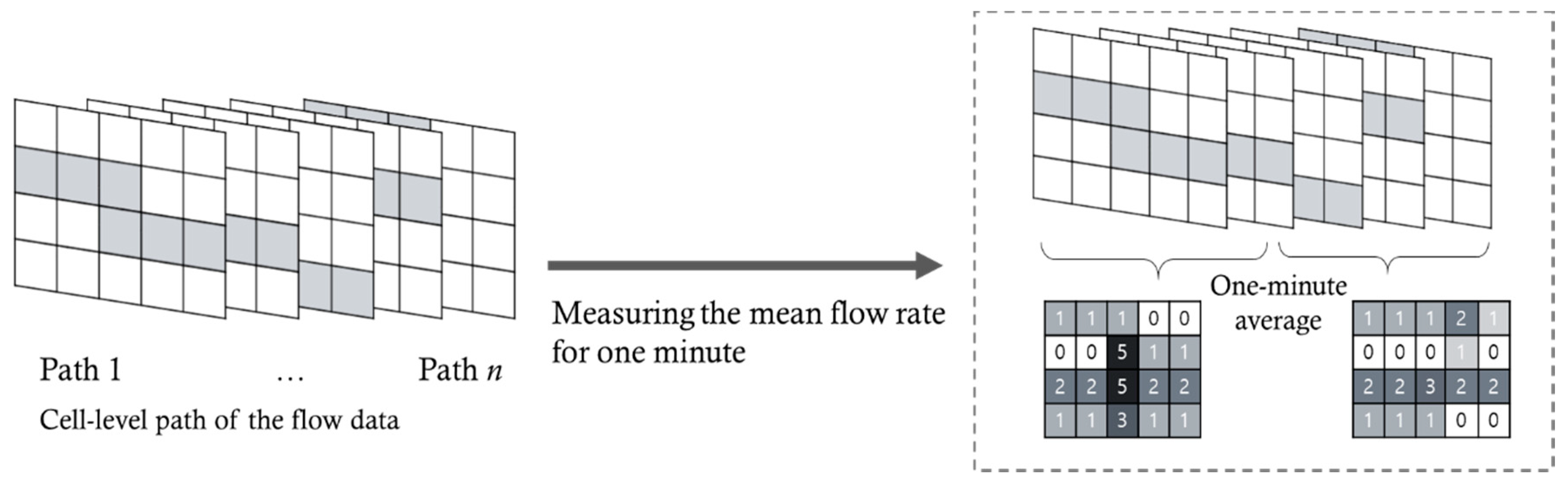
For the walking space’s configuration, we divide the walking space into cells, in which the size is set to the average walking distance for one second. Then, a section is defined as the group of cells in m columns and $n$ rows. The path selection behavior of pedestrians is numerically measured and compared based on the section.

The subject pedestrian data are selected and used to analyze the path planning behavior of subject pedestrians. The remaining trajectory data are used to generate flow data to represent the subject pedestrians’ dynamic walking environment. Following the space configuration, we present the trajectory data as an ordered set of consecutive cells, as shown in Figure 2. The direction of flow is defined as N-S-E-W, and each directional flow rate is measured for each cell every minute.

3.1. Identification of Influential Flow Conditions of Path Selection

This section investigates the influential flow conditions on pedestrians’ path selection behavior. We first define three types of flow conditions consisting of pedestrians located in the direction of the subject’s destination: $Q_0,Q_1,\mathrm{and}{Q}_2$, as shown in Figure 3. $Q_0$ includes all direction flows. $Q_1$ excludes pedestrians walking in the same direction as the subject pedestrian in $Q_0$. $Q_2$ includes only pedestrians who are walking in the opposite direction to subject pedestrians. These three conditions all include opposite direction flow of subject pedestrians, and as it moves from $Q_0$ to $Q_2$, the proportion of the opposite direction flow increases. In addition, we classify each flow condition into a high flow condition $Q_i^{high}\left(i=0,1,2\right)$ and a rest condition $Q_i^{rest}\left(i=0,1,2\right)$ based on the 75th percentile of flow distribution over space and time.

As shown in Figure 4, we measure the changes of path under different flow conditions to compare the influence of the high flow conditions of $Q_0,Q_1,\mathrm{and}{Q}_2$ on path selection with the rest of the flow conditions. Using the path data, we can measure the rate of cell choice $R_{high}\left(i,j\right)$ and $R_{rest}\left(i,j\right)$ for each $Q_0,Q_1,\mathrm{and}{Q}_2$ as

$$R_{high}\left(i,j\right)=\frac{N_{high}\left(i,j\right)}{{{\displaystyle \sum }}_{j^{\prime }=1}^n{N}_{high}\left(i,j^{\prime }\right)},$$

(1)

$$R_{rest}\left(i,j\right)=\frac{N_{rest}\left(i,j\right)}{{{\displaystyle \sum }}_{j^{\prime }=1}^n{N}_{rest}\left(i,j^{\prime }\right)},$$

(2)

where $N_{high}\left(i,j\right)$ denotes the number of pedestrians who pass the $j\mathrm{th}$ row of the $i\mathrm{th}$ column under the high flow conditions. As $n$ denotes the number of rows, ${\displaystyle \sum }_{j=1}^n{N}_{high}\left(i,j\right)$ is the total number of pedestrians who pass the $i\mathrm{th}$ column. Note that ${\displaystyle \sum }_{j=1}^n{R}_{high}\left(i,j\right)=1$ and ${\displaystyle \sum }_{j=1}^n{R}_{rest}\left(i,j\right)=1$. The most frequently chosen path is defined as the ordered set of cells in each column, and the second most frequently chosen path is defined from the set of remaining cells. We can get the rest of the paths in a similar manner which is as many as the number of rows. After calculating $R_{high}\left(i,j\right)$ and $R_{others}\left(i,j\right)$ from (1) and (2), one can obtain the empirical probability mass function of the average rate of cell choice, ${\overline{R}}_{high}\left(j\right)$ and ${\overline{R}}_{others}\left(j\right),$ as follows:

$${\overline{R}}_{high}\left(j\right)=\frac{1}{m}{\displaystyle \sum }_{i=1}^m{R}_{high}\left(i,j\right),j=1,\dots , n,$$

(3)

$${\overline{R}}_{rest}\left(j\right)=\frac{1}{m}{\displaystyle \sum }_{i=1}^m{R}_{rest}\left(i,j\right),j=1,\dots , n,$$

(4)

where ${\overline{R}}_{high}\left(j\right)$ and ${\overline{R}}_{rest}\left(j\right)$ in (3) and (4) are the probability distribution that subject pedestrians choose the cells in the $j\mathrm{th}$ row. Using ${\overline{R}}_{high}\left(j\right)$ and ${\overline{R}}_{rest}\left(j\right)$, we measure the difference in the distribution of the cell choice under high flow conditions and the rest of the conditions in Kullback–Leibler divergence,$D_{KL}$. Figure 4 shows how the rate of cell choice and $D_{KL}$ are obtained. The difference of pedestrians’ statistical behaviors between different opposite flow rates can be measured by $D_{KL}\left({\overline{R}}_{high},{\overline{R}}_{rest}\right),$ which is defined as

$$D_{KL}\left({\overline{R}}_{high}, {\overline{R}}_{rest}\right)\triangleq {\displaystyle \sum }_{j=1}^n{\overline{R}}_{high}\left(j\right)\log \left(\frac{{\overline{R}}_{high}\left(j\right)}{{\overline{R}}_{rest}\left(j\right)}\right),$$

(5)

where $D_{KL}\left({\overline{R}}_{high}, {\overline{R}}_{rest}\right)\ge 0$. It shows the difference of two distributions in (5), measuring the path-choice pattern changes under the high flow conditions compared to the rest conditions.

3.2. Analysis on the Spatial and Temporal Range of the Flow Condition

This subsection aims to find spatial and temporal influential ranges of the opposite flow on path selection and update behavior. The spatial influential ranges refer to the average distance of the opposite flow influencing the path planning behavior. The temporal influential range is the average time that affects the path planning behavior after the opposite flow appears within the spatial influential range of the pedestrian. Although these ranges are the key parameters of path planning behavior models, only a few studies noted the influential ranges of flow [5,6,7,8,9,10,11,12,23]. In this study, the spatial range is first identified, then the temporal range is determined from the empirical data.

To investigate the spatial influential range of the opposite flow, we define the flow conditions $Q_0^{\left(r\right)},Q_1^{\left(r\right)},\mathrm{and}{Q}_2^{\left(r\right)}$, where the superscript $\left(r\right)$ indicates the range of pedestrians as shown in Figure 5. Then, we define ${\overline{R}}_{high}^{\left(r\right)}$, ${\overline{R}}_{rest}^{\left(r\right)}$, and $D_{KL}\left({\overline{R}}_{high}^{\left(r\right)},{\overline{R}}_{rest}^{\left(r\right)}\right)$ for each flow condition $Q_0^{\left(r\right)},Q_1^{\left(r\right)},\mathrm{and}{Q}_2^{\left(r\right)}$. The $D_{KL}\left({\overline{R}}_{high}^{\left(r\right)},{\overline{R}}_{rest}^{\left(r\right)}\right)$ shows the level of path changes under the high flow rate of $Q_0^{\left(r\right)},Q_1^{\left(r\right)},\mathrm{and}{Q}_2^{\left(r\right)}$ compared to the rest of the flow rate.

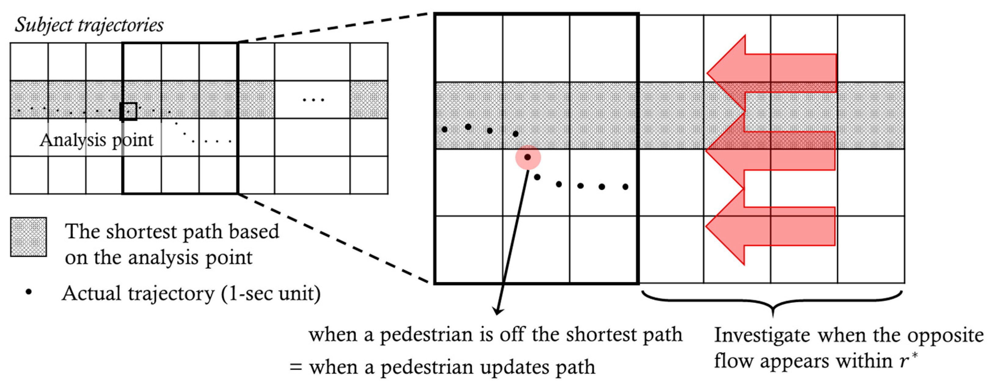
Next, we propose a method for identifying the temporal influential range with a given flow condition and its spatial influential range, as illustrated in Figure 6. We assume that pedestrians prefer the shortest path, and they update their paths outside a certain range from the shortest path when they face the opposite flow. From the relationship between the time of opposite flow and the time of updating path, we can remark that the opposite flow is a factor that makes pedestrians update their paths. In addition, we can find the temporal influential range of the flow. Here, we set the pedestrian’s destination to the last point of his/her trajectory, and then the shortest-distance path can be obtained.

4. Experiments

4.1. Dataset

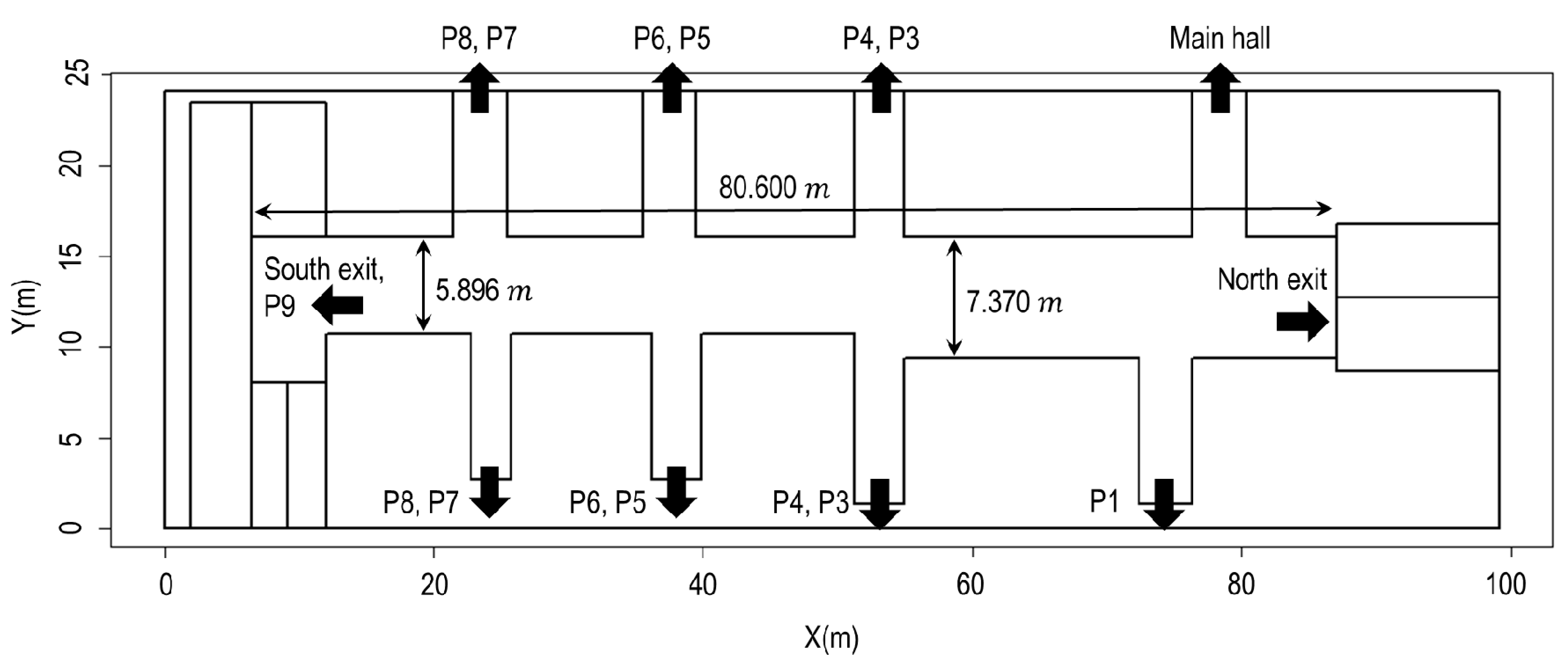
The dataset was collected in the west passage of the Lausanne train station on 27 February 2013. It was collected by a large-scale network of infrared and depth sensors deployed in the station. The west passage is the main passage of Lausanne station connecting to major cities in Switzerland, often crowded with many pedestrians. Figure 7 shows the layout of the data site. This study’s analysis region is the central aisle. The central aisle is connected to the North exit, Main hall, platforms, and South exit from the right side to left side. The length of the aisle is 80.6 $\mathrm{m}$ and the width of the aisle is 7.370 on its first half and narrows to 5.896 $\mathrm{m}$ on the second half.

To collect the raw data, large-scale network of smart sensors, consisting of infrared and depth sensors, has been installed on the Lausanne train station. When pedestrians appear in the scene covered by the sensor network, each pedestrian’s silhouette is detected. The trajectory data are generated by linking the detected pedestrians over the network of sensors.

The raw data includes 6928 pedestrian trajectories for 88 min during the morning peak hours. Each trajectory consists of pedestrian ID and two-dimensional coordinates indicating the detected locations along with time. The time resolution is 0.1 s. The average length of the trajectories is 64.18 $\mathrm{m}$, and the average duration of a pedestrian stay is 60.68 s. The average speed is 1.35 $\mathrm{m}/\mathrm{s}$.

4.2. Data Processing

We preprocess the raw data in two steps. First, to identify causal factors of path planning and to analyze the spatial range of causal factors, we convert the trajectory data into cell-level paths, as explained in Section 3.1. The cell size is set to $1.4\mathrm{m}\times 1.4\mathrm{m}$ based on the average speed of pedestrians. We divide the area with a width of $5.9\mathrm{m}$ into four rows of cells and the area with a width of $7.4\mathrm{m}$ into five rows of cells. Second, we aggregate the data in the form of one-second unit trajectories to analyze the temporal range of causal factors in Section 3.2.

The trajectory data for 88 min are categorized into subject data and flow data as mentioned in the previous section. We choose the pedestrians’ trajectories who move to the south exit/P9 from the main hall, which is the most in-demand subject data. The trajectories of the remaining pedestrians are set to the flow data. The subject and flow data are divided into 88 subsets of one-minute-long data.

The pedestrians’ trajectories, moving to the south exit and P9 from the main hall, are set as the subject data, whose direction is ‘From right to left.’ In the case of flow data, the trajectories’ direction of pedestrians who move from $\mathrm{O}\in${Main hall, North exit, P1, P3, P4, P5, P6} to D$\in${P7, P8, P9, South exit} is ‘From right to left,’ which is the same as the subject pedestrians. The trajectories’ direction of pedestrians who move from $\mathrm{O}\in$ {P7, P8, P9, South exit} to $\mathrm{D}\in$ {Main hall, North exit, P1, P3, P4, P5, P6} is ‘From left to right’, which is the opposite to the subject pedestrians.

Using the cell-level paths of the flow data, we measure the average flow for each cell. For the analysis on the temporal range of causal factors, we use the one-second average flow. For the rest of the studies, we use the one-minute average flow.

4.3. Results

This section presents the analysis result of the methodologies described in Section 3.1 and Section 3.2.

4.3.1. Identification of Influential Flow Conditions of Path Selection

Some literatures on path planning behavior of pedestrians have showed that one of the main factors of the behavior changes is the high flow [4,7]. To investigate the influence of the opposite flow on the path planning behavior with the empirical data, we compare paths selected by subject pedestrians when they face different flows as described in Figure 3. In this study, when preprocessing the pedestrian trajectory data, we classify the flow distribution into four levels: High flow (75th percentile), Mid-high flow (50th percentile), Mid-low flow (25th percentile), Low flow (the rest). Then, we grouped Mid-high flow (50th percentile), Mid-low flow (25th percentile), and Low flow (the rest) as the normal flow group. If the flow rate is beyond the 75th percentile of flow distribution, we classify it as a high flow rate, if not, it is considered as others. The criteria for classification can be changed according to the analysis purpose. If the pedestrian behavior in more extreme situations needs to be observed, the criteria can be adjusted to be higher. From the dataset used, the 75th percentile values of the average flow rate on the entire central aisle are $Q_0:$15.65 (peds/${\mathrm{m}}^2 \min$), $Q_1:$5.52 (peds/${\mathrm{m}}^2 \min$), and $Q_2:$4.14 (peds/${\mathrm{m}}^2 \min$). We use the three most frequently chosen cells among the five cells belonging to each column to determine each case’s frequently chosen paths.

The paths frequently chosen in high flow are shown in Figure 8, and the paths frequently chosen in the other cases are shown in Figure 9. The subject pedestrians tend to move from the upper-right to the middle-left side since they are heading towards the South exit or P9 from the main hall. In other cases, the difference is negligible between the paths chosen by subject pedestrians when facing $Q_0, Q_1, \mathrm{and}{Q}_2$. From Figure 9, one can notice that pedestrians usually walk to the center of the aisle when they leave the main hall and walk straight. However, as the flows become high, the subject pedestrians tend to stick to the right wall for a longer time immediately after leaving the main hall, regardless of the flow directions. Furthermore, this tendency gets more evident in the order of $Q_0, Q_1, \mathrm{and}{Q}_2$. The results show that if the proportion of the opposite flow is high, there are more changes in the path selection decision.

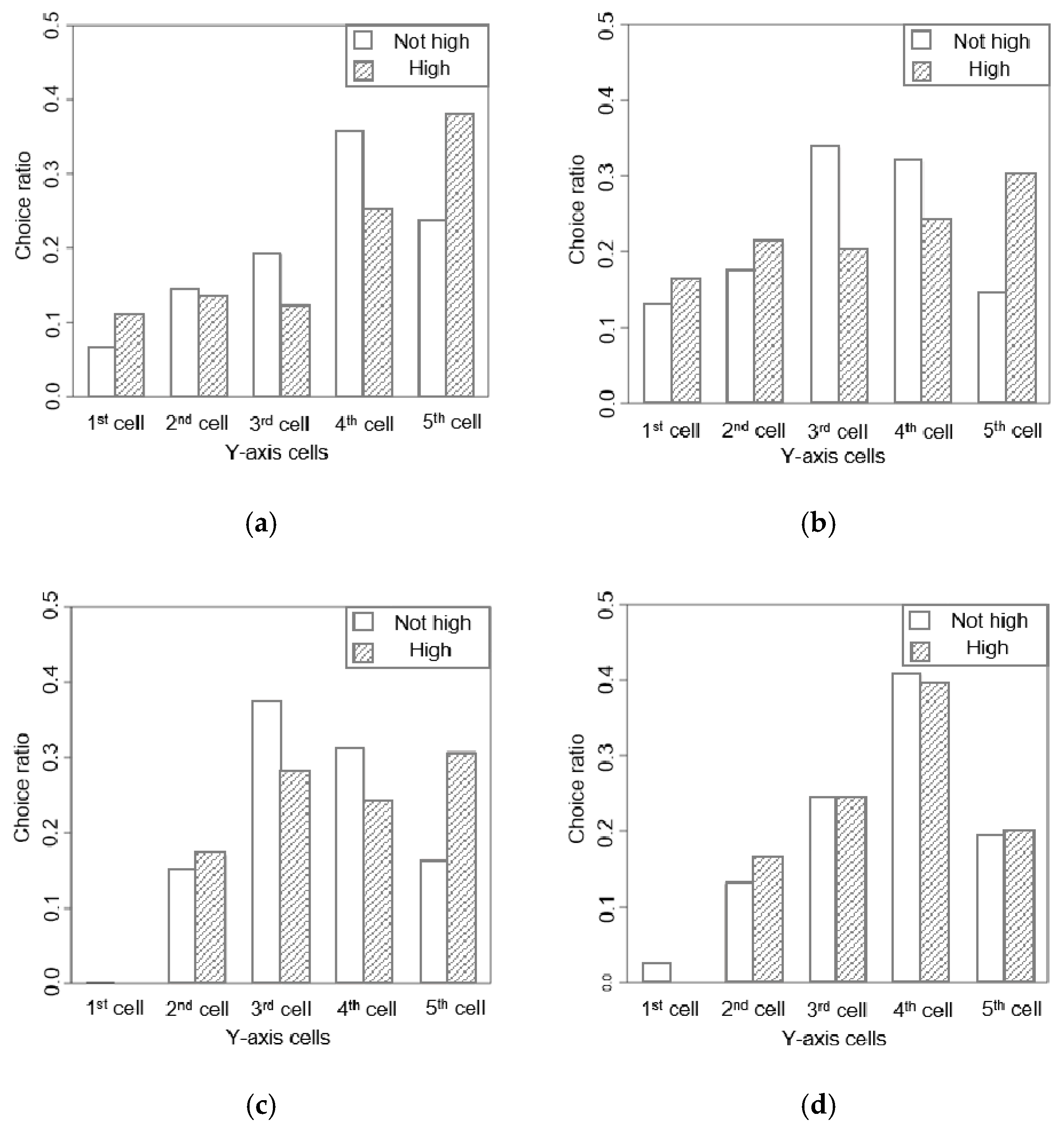
In order to analyze the changes in path selection behavior by the opposite flow in more detail, we measure ${\overline{R}}_{high}\left(j\right)$ and ${\overline{R}}_{r\mathrm{est}}\left(j\right), j=1,\dots , 5$ and $D_{KL}\left({\overline{R}}_{high},{\overline{R}}_{others}\right)$ of the opposite flow $Q_2$ for sections of the central aisle. There are four sections, and each section is composed of 12 columns and 5 rows. Figure 10 shows the sections’ configuration. The probability distribution ${\overline{R}}_{high}\left(j\right)$ and ${\overline{R}}_{r\mathrm{est}}\left(j\right)$ of each section is shown in Figure 11, and the value of $D_{KL}\left({\overline{R}}_{high},{\overline{R}}_{others}\right)$ of each section is shown in

Table 2. Mean probability distribution of cell choices by subject pedestrians.

	Section 1	Section 2	Section 3	Section 4
$D_{KL}$	0.08	0.10	0.04	0.02

.

Bar plots in Figure 11 show two distributions of the mean probability of cell selection in each row. The white bar plots represent the pedestrians facing high opposite flows, and the gray bar plots show the remaining cases. In the first section, pedestrians often choose the 4th cell and the 5th cell since they enter the central aisle through them. In particular, when there is a high opposite flow, many pedestrians select the upper cells to move along the right wall. One can see from Table 2 that the $D_{KL}$ value of Section 1 is the second largest among the four sections, which indicates that the difference in path choice behavior is relatively high when pedestrians face high flow and when they do not. Next, in Section 2 and Section 3, pedestrians tend to pass through the center of the aisle when the opposite flow is not high, and they tend to move along the right wall when the opposite flow is high. $D_{KL}$ values in Table 2 show that the difference in path selection behaviors with respect to the rate of the opposite flow is the largest in Section 2. Lastly, there is no significant difference in path selection behaviors concerning the opposite flow in Section 4, as seen in Figure 11d and $D_{KL}$ values in Table 2.

The subject pedestrians move from the main hall to the South exit or P9, where the first section is near the origin and the fourth section is near the destination. Accordingly, the difference in $D_{KL}$ between sections shows that pedestrians’ path selection behavior changes depending on the distance to the origin or destination. Previous studies on path planning behavior have focused on the effect of the distance and relative moving direction between pedestrians, as shown in Table 1.

4.3.2. Analysis on the Spatial and Temporal Range of the Flow Condition

As we mentioned in Section 3.2, to analyze spatial and temporal influential ranges, we measure $D_{KL}\left({\overline{R}}_{high}^{\left(r\right)},{\overline{R}}_{others}^{\left(r\right)}\right)$ under $Q_0^{\left(r\right)},Q_1^{\left(r\right)},\mathrm{and}{Q}_2^{\left(r\right)}$. The results are shown in Figure 12. In the case of opposite flow, as $r$ increases to $30.95 \mathrm{m}$, the value of $D_{KL}\left({\overline{R}}_{high}^{\left(r\right)},{\overline{R}}_{others}^{\left(r\right)}\right)$ also steadily increases, resulting in a maximum value of 0.21. After that, as $r$ increases to $56.46\mathrm{m}$, it decreases to 0.13, and then remains flat. The result implies that the critical spatial range that leads pedestrians to change their paths is $r=30.95 \mathrm{m}$, while opposite flow still affects pedestrians up to 56.46 $\mathrm{m}$, which is the maximum influential range. Meanwhile, in the other direction flows, $D_{KL}\left({\overline{R}}_{high}^{\left(r\right)},{\overline{R}}_{others}^{\left(r\right)}\right)$ does not show clear tendency with respect to $r$.

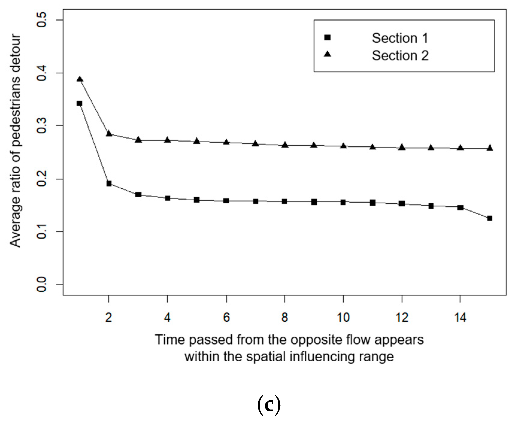
Next, the temporal range of path planning is measured by the time gap between the moment when the opposite flow appears within the spatial range $r=30.95 \mathrm{m}$ and the path update. To analyze different behaviors during the progress of trips, we measure each section’s time gap in the aisle. Only the 1st and 2nd sections where the distance to the destination is longer than $30.95 \mathrm{m}$ are analyzed. We assume that pedestrians’ behavior of deviating from the shortest path is from the path updating action to avoid the opposite flow. Accordingly, the pedestrian updates his/her path at the moment when he/she moves to the cell out of the shortest path. We analyze cases with more than three pedestrians to reduce errors, with at least one pedestrian who updates his/her path.

The results are shown in Figure 13. In the first section, the ratio of the pedestrian updating his/her path within 1 s after the opposite flow appears within $r=30.95 \mathrm{m}$ is between 0.3 and 0.4, and the ratio falls below 0.2 after 2 s. The 2nd section has a higher rate of path update than the 1st section and, as the opposite flow rate increases, the path update ratio also tends to increase. Moreover, the path update’s temporal range is analyzed to be 2 s, as in the 1st section. We can see that pedestrians are affected by the opposite flow and updated their paths within 1 to 2 s.

We analyze the spatial and temporal ranges of the opposite flow that affect the path update behavior from the previous results. The spatial influential range that affects the most pedestrians to update their paths is $30.95 \mathrm{m}$. In the previous studies, the ranges affecting pedestrians’ path update behavior were not specified. Previously, it was assumed that the pedestrian reacts to changes in their visibility range or their walking space and update their path in the next time step [1,4,5,6,7,8,9,10,11,12], which shows that the path planning/update behavior modeling lacks consideration of the spatial and temporal range. Although the maximum influential distance for collision avoidance in some modelling studies is assumed to be 10–20 m [23,24], we find that the opposite flow affects pedestrians over a wider range of spaces. This implies that the tactical-level decision is based on a wider range of environmental information than that on the operational level.

Finally, we measure the pedestrian’s path updating ratio with respect to the opposite flow rate that appears within the spatial and temporal ranges. The result is shown in Figure 14 and

Table 3. The ratio of path update with respect to the opposite flow rate and its fitted curve.

Percentile of the Rate of the Opposite Flow	The Average Rate of Opposite Flow $(\mathbf{p}\mathbf{e}\mathbf{d}\mathbf{s}/{\mathbf{m}}^2\mathbf{s})$	The Rate of Pedestrians’ Path Update
90%	3.22	5.08%
80%	3.86	4.76%
70%	4.84	4.96%
50%	6.44	5.57%
30%	7.76	6.32%
10%	8.08	7.49%
5%	8.53	16.61%
1%	8.91	24.06%

. Figure 14 shows the ratio of path update with respect to the opposite flow rate. One can note that when the opposite flow rate is less than 8 $\mathrm{peds}/{\mathrm{m}}^2\mathrm{s}$, the path update ratio increases to 5%. When the opposite flow rate is greater than 8 $\mathrm{peds}/{\mathrm{m}}^2\mathrm{s}$, it increases noticeably.

5. Conclusions

This paper introduces a new methodology for investigating dynamic walking conditions that influence pedestrians’ path selection decisions. The influential flow conditions of path selection decisions are first identified, then their spatial and temporal ranges are investigated. The comparison with the paths of subject pedestrians who face different flow conditions shows that the opposite flow affects pedestrians’ path selection decision more than other direction flows. It is also found that the higher the proportion of opposite flows, the greater the influence of the path selection decision. We also find that the distance they have walked from the origin and the distance to the destination affects the flow’s influence level. Then, the investigation on the spatial and temporal ranges of the opposite flow follows. The level of changes in path selection decision with respect to the opposite flow rate shows that most pedestrians consider about 30 m in advance to plan their paths. The relationship between the time of opposite flow occurring and the time of updating path shows that the temporal range of opposite flow is less than 2 s.

Nevertheless, the experiment results presented in this paper are based on one dataset acquired in the Lausanne station. As many other factors beyond this dataset influence the human decision process, the findings from this research cannot be directly transferred to other sites or cases. Therefore, to generalize this research’s findings, we need to conduct more empirical studies of diverse situations in future. As this study is one of the first efforts revealing path update behavior, our further research will focus on behavior modelling under dynamic conditions.