1. Introduction
Traffic, energy, and environmental infrastructure (including bridge structures) represent approximately 70% of the national property in European countries. Their operation, maintenance, and repairs require approximately 35% of the overall material and energy needs and produce roughly 30% of all waste and environmental burdens. The primary factors affecting the conditions of the operated bridge structures include not only natural changes to materials, hidden structural defects, and increased intensity of traffic but also degradation processes that occur in structural elements due to the environmental stress caused by the surrounding environment [
1,
2]. The negative impact of the degradation processes can be documented on the technical conditions of road bridges in the Czech Republic: out of the total of approximately 16,000 operated bridge structures in the Czech Republic, roughly 1000 are in a very poor or emergency condition [
3,
4,
5].
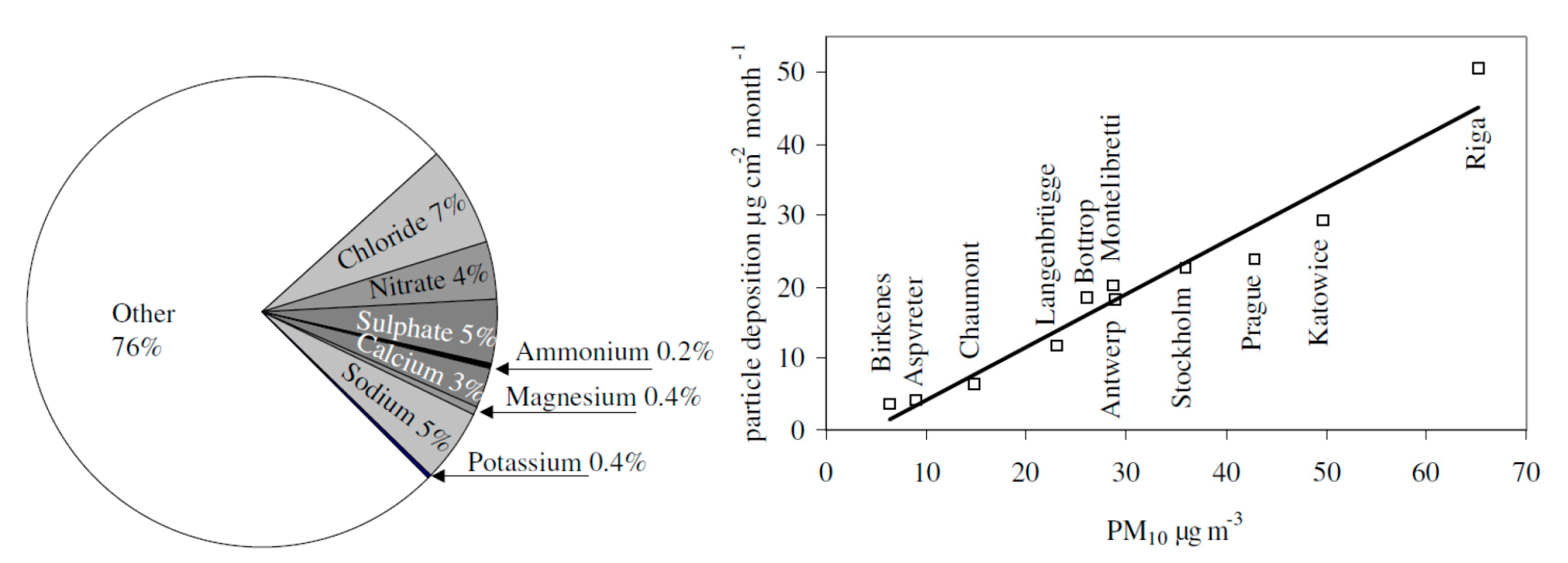
Air pollution is one of the primary degradation factors that affect the required durability of bridge structures. Air pollution affects the degradation of most materials used in traffic infrastructure (for steel elements this is notably related to damage caused to the corrosion protection system, leading to corrosive damage). Air pollution can be caused by two sources: natural sources or human activities; the latter is becoming increasingly prevalent. The surroundings of roads with intense road traffic characteristically feature specific microclimatic conditions, notably including a higher concentration of settled dust particles and chloride ions from the de-icing salts used for winter maintenance.
Basic environmental parameters affecting degradation processes notably include temperature, air humidity, precipitation and its pH, air pollution notably including the deposition of sulfur dioxide, nitrogen oxide and chlorides, dust particles, and others [
6,
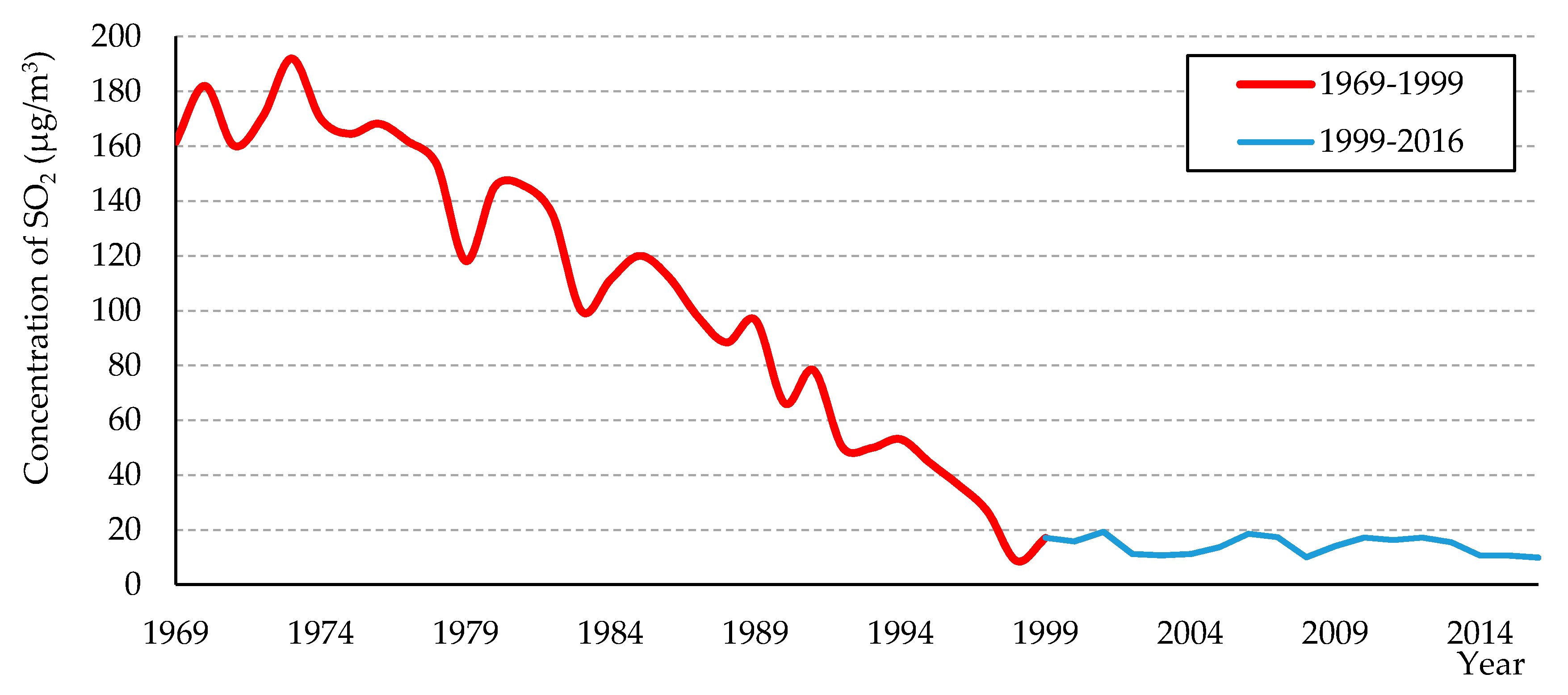
7]. The degradation of the surfaces of steel structures is significantly influenced by two corrosion stimulators related to air pollution: the effects of sulfur dioxide and the depositing of chloride ions. The concentration of SO
2 in the air reached its peak in the Czech Republic (similarly as elsewhere in Europe) in the seventies and eighties of the previous century. At that time, the air concentration of SO
2 in the Czech Republic reached up to 200 μg/m
3 [
6,
7]. A significant drop in the concentration of SO
2 was caused primarily by the introduction of desulfurizes in large industrial companies. Currently, the SO
2 concentrations in the Czech Republic fluctuate at around 10 μg/m
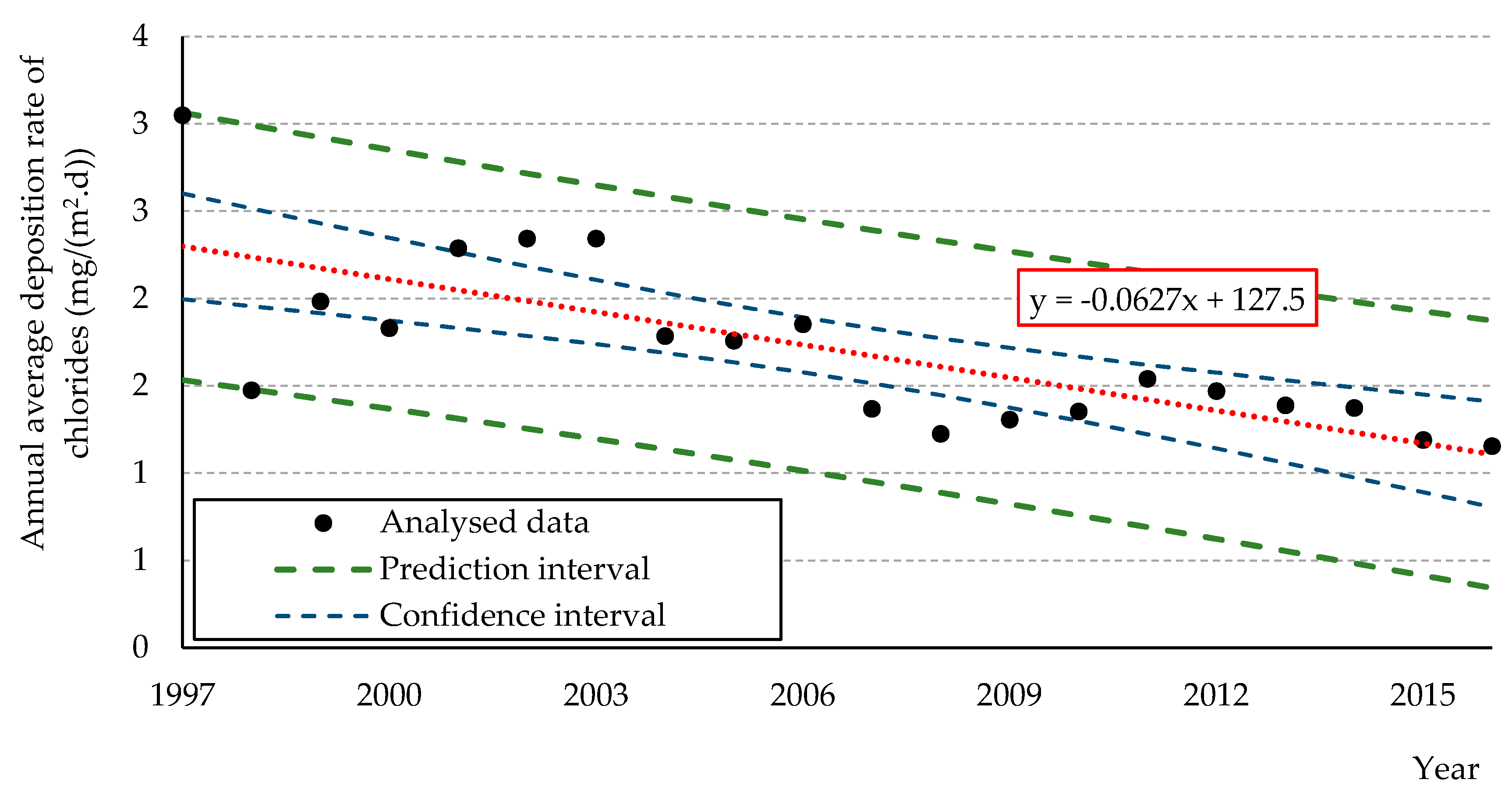
3. On the other hand, the amount of settled chloride ions in the vicinity of roads exhibits an opposite trend, with an increase caused by the higher intensity of road traffic. Chloride ions spread together with the aerosol from melting ice or dust to the surfaces of structures from chemical de-icing agents used during the winter maintenance of roads. The spread of chlorides is significant especially on a local scale, near the vicinity of roads, depending on the parameters of the surrounding environment, the quantity and nature of barriers located in the vicinity of the road, speed and intensity of traffic, etc. [
8,
9,
10]. Experimental measurements carried out at selected bridge structures and in their surroundings called attention to the fact that the quantity of deposited chloride ions spread in the air is also significantly impacted by the design of the bridge structure and the topography of the surrounding terrain [
11,
12,
13].
A good estimate for the corrosive behavior of metal in the atmosphere is one of the key parameters allowing the design of suitable measures (selection of a corrosion protection system, suitable dimensions for profiles, structural solutions that match the environmental conditions, functional maintenance system) that will allow for the reliable operation of load-bearing elements of the bridge structure for its whole planned service life. The corrosion aggressiveness of the atmospheres (the environment) is usually related to the value of expected corrosion losses. The effects of atmospheric corrosion can be described using a model that considers the environmental parameters that affect the corrosive behavior of metals in the following general form [
6,
14,
15]:
where
Kdry represents the set of effects of basic parameters for dry atmospheric deposition on the structure’s surface and
Kwet represents the set of effects of basic parameters for wet atmospheric deposition on the structure’s surface.
The environment where the structure is located can be classified into one of several corrosion classes (C1 to CX) based on the corrosion rates,
rcorr, measured after 1 year of exposure (whereas the pollution factors and limits are available in EN ISO 9223 [
16]).
The corrosivity category (i.e., the corrosion rate) of the atmosphere can be determined in several ways:
Experimental measurements obtained via exposed corrosion coupons;
Experimental measurements utilizing resistance sensors;
Estimations based on classified intervals of environmental parameters;
Calculation of corrosion losses from dose–response functions based on the knowledge of the required environmental parameters;
Derived maps of the environment’s corrosion aggressiveness.
The method of determining atmospheric corrosivity via exposed corrosion coupons directly captures the conditions at the considered site but is also highly demanding in terms of time. An alternative is to measure the environment’s corrosivity via resistance sensors; however, these are usually designed to be used only in inside areas [
17,
18,
19]. The most used and easily accessible methods for determining the corrosivity of the atmosphere, i.e., for estimating the corrosion rate
rcorr after 1 year of exposure, is the use of previously derived regression formulas, notably dose–response functions. These formulas were obtained for individual types of metals based on long-term experimental evaluations [
15,
16,
20,
21]. For carbon steel, it is possible to use one of the following dose–response functions (the same function can also be used for weathering steel):
- (A).
Dose–response function according to EN ISO 9223 [
16]
The corrosion loss for carbon steel after 1 year of exposure is governed by the following empirical formula:
where
is defined as
, assuming that the average air temperature is below 10 °C, otherwise the equation is defined as
;
Pd is the average annual deposition of SO
2 (mg/(m
2·d));
Sd is the average annual deposition of Cl
− (mg/(m
2·d));
T is the average annual temperature (°C), and
RH is the average annual relative humidity (%).
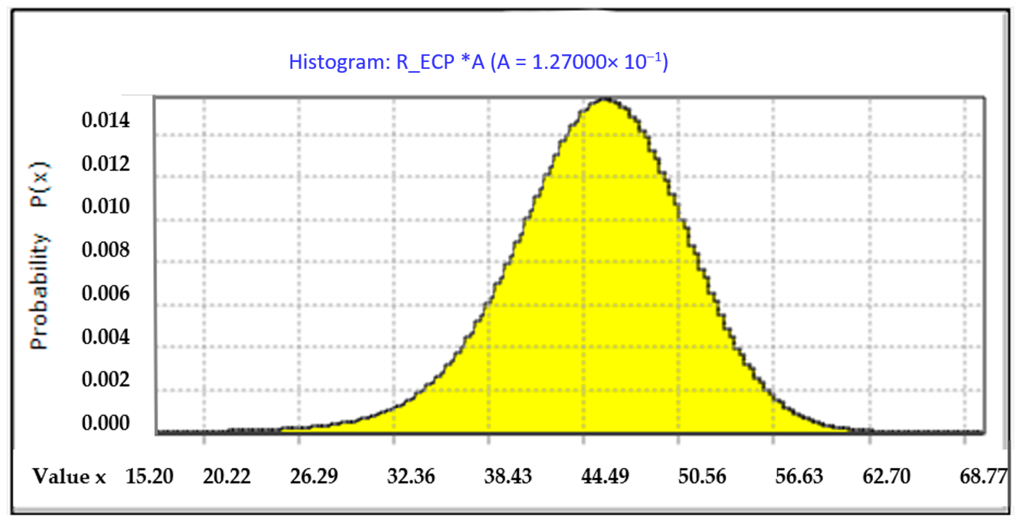
- (B).
Dose–response function according to experimental tests from the UN/ECE ICP project on the Effect on Materials [
20]
The UN/ECE ICP project was carried out between 1987 and 1995 [
20]. The program shows that the corrosion loss of weathering steel can be estimated using the following empirical formula:
where
is defined as
, assuming that the average air temperature is below 10 °C, otherwise the equation is defined as
;
Pd is the average annual deposition of SO
2 (mg/(m
2·d));
T is the average annual temperature, and
RH is the average annual relative humidity (%).
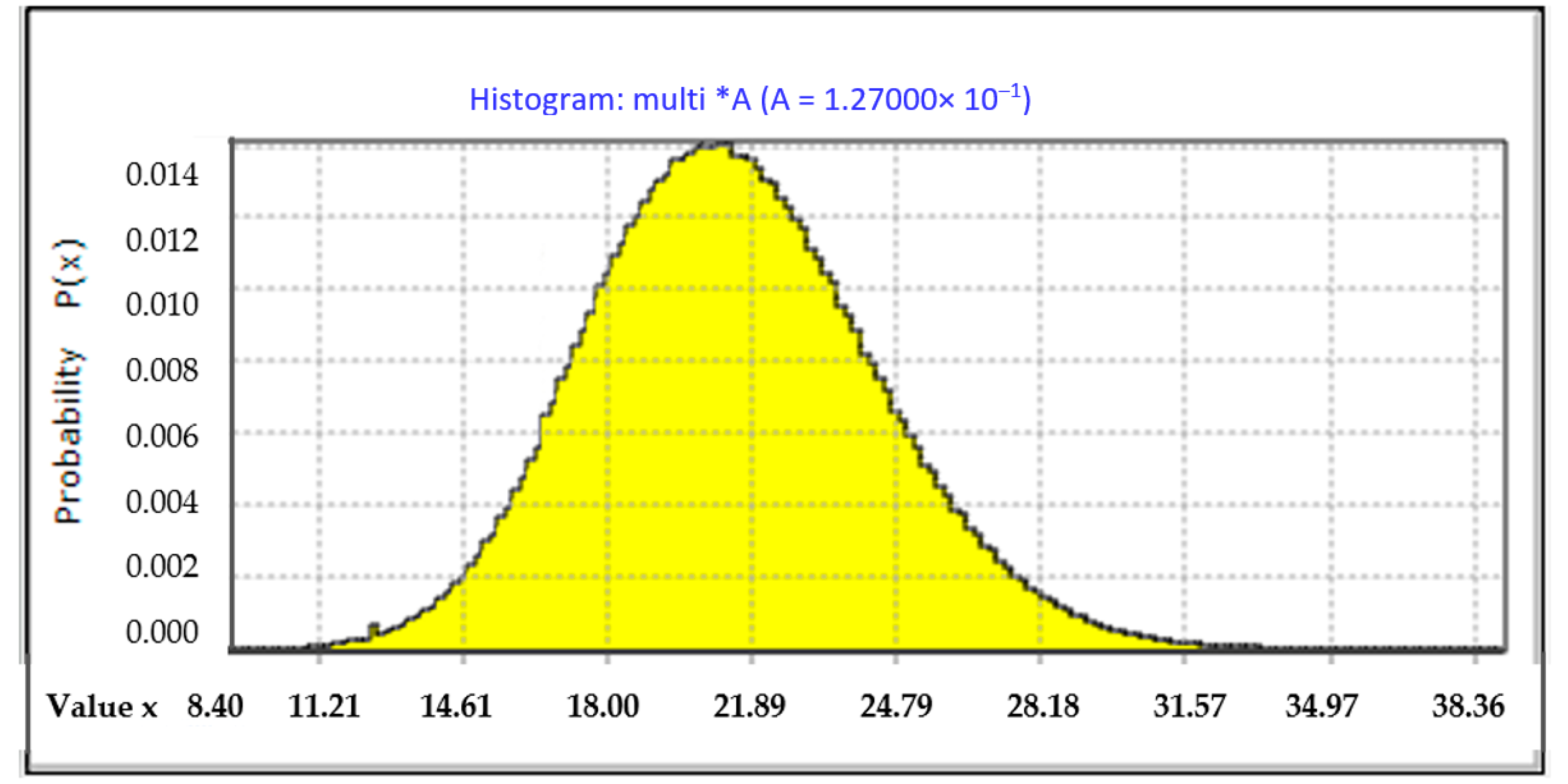
- (C).
Dose–response function according to experimental tests from the Multi-Assess program [
21]
This program involved the placement of corrosion coupons at 50 test sites in Europe [
21]. The samples (coupons) used to estimate corrosion losses considered significantly more environmental parameters than the equation listed above. The experimental test period already includes a significant drop in the primary corrosion stimulator in the air, notably sulfur dioxide. Based on this program, the corrosion loss of carbon steel can be predicted using the following empirical formula [
21]:
where
is defined as
, assuming that the average air temperature is below 10 °C, otherwise the equation is defined as
;
. is the average annual deposition of SO
2 (mg/(m
2.d));
Sd is the average annual deposition of Cl
– (mg/(m
2.d));
RAIN is the average annual precipitation (mm);
RH60 is the average relative humidity (%); H
+ is the average annual pH of precipitation, and
PM10 is the average annual concentration of dust particles (maximum diameter of 10 µm) (µg/m
3).
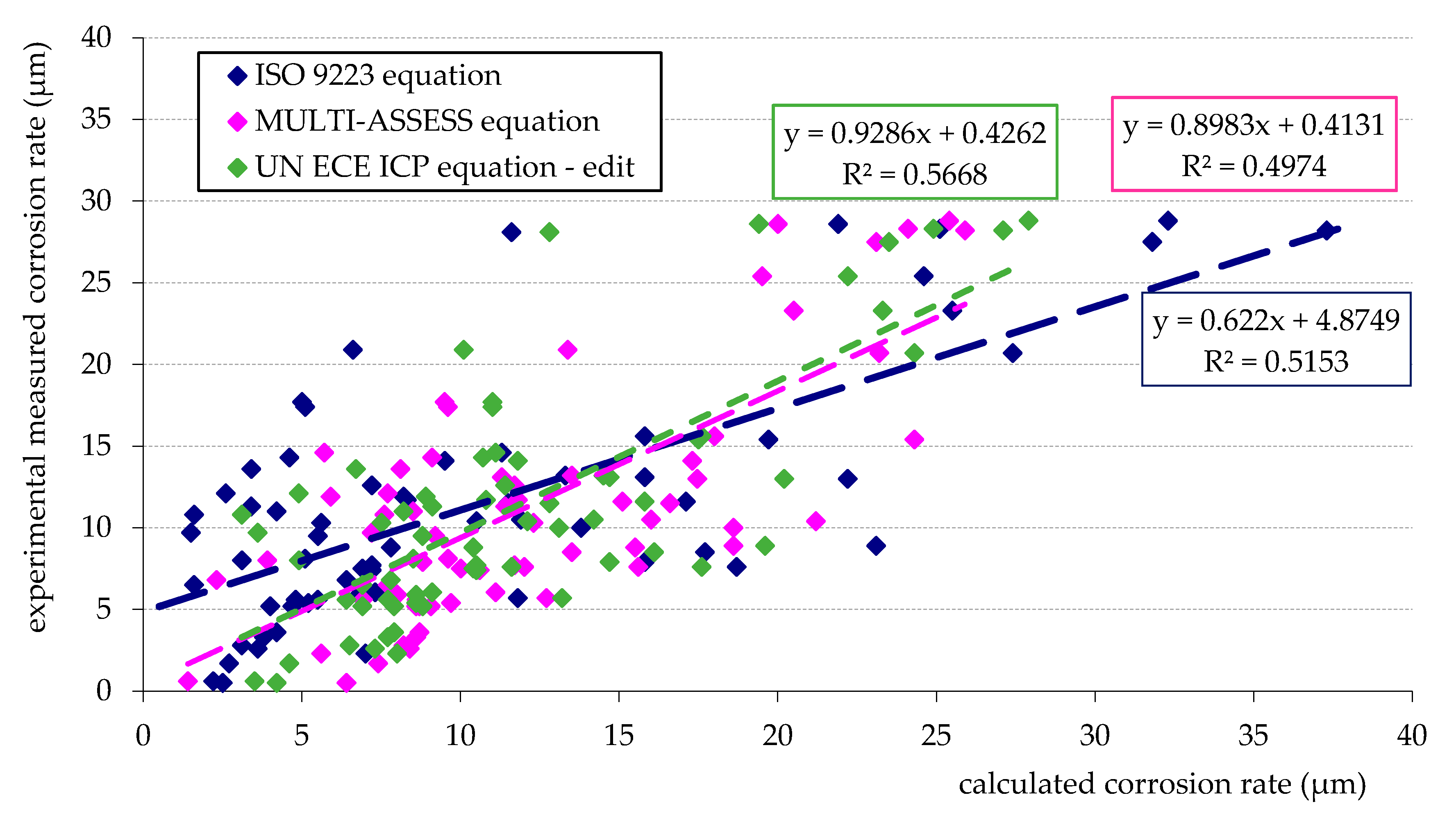
The corrosion losses calculated using the prediction models listed above were compared to the actual corrosion losses of carbon steel determined in 2005/06, 2008/09, and 2011/12 within the UN/ECE ICP program for atmospheric stations in Europe (
Figure 1). It is important to mention that mathematical prediction models are mere approximations, that they are simplified, and are burdened with significant insecurities. However, the values listed in the figure indicate that the simplified formulas take into account the trend dependency rather well, but the results do exhibit a significant variance. In addition to the insecurities arising from the use of a specific prediction model, the variability of the predicted corrosion rates is also significantly affted by the random and variable nature of environmental parameters, which form input parameters in the appropriate dose–response functions.
The article introduces and evaluates a stochastic approach to predictive models, which allows us to consider the random and variable nature of the input environmental parameters with sufficient accuracies, while also respecting the recommendations arising from long-running corrosion programs. The article also provides the results of sensitivity analyses that can be used to evaluate the specific impacts of individual corrosion agents on corrosion damage to structures. Special attention was also paid to sensitivity analysis focusing on an assessment of the impact of chloride deposition on corrosion damage to steel bridge structures. The analysis utilized data obtained from experimental measurements of deposition rates of chlorides in the vicinity of roads operated in the Czech Republic.
The main objectives of the article can be summarized in the following points:
▪ A procedure for stochastic processing of long-term measured environmental data;
▪ Introduction of a probabilistic prediction model for calculation of annual corrosion loses;
▪ Verification of suitable equations (so-called dose–response functions) for probabilistic prediction models of corrosion damage of steel structures in the vicinity of roads;
▪ Influence of individual environmental parameters on corrosion damage;
▪ A study focused on the specifics of corrosion damage to steel structures near roads where de-icing salts are used.
Probabilistic approaches are increasingly used to assess the reliability of building structures [
22]. Using probabilistic methods, it is possible to directly take into account the random variability of input variables in the calculation. Typical random variables are material characteristics (especially the yield strength in structural steel) and individual loads acting on the structure (dead and live loads, snow, wind, and temperature loads, or traffic loads). The influence of the environment is a specific action, which manifests itself in steel structures mainly by their corrosion damage. Accurate prediction of corrosion damage will provide structural engineers and researchers with the necessary data to evaluate the durability of building structures [
1,
2,
3]. Probabilistic calculations also make it possible to evaluate the impact of specific environmental factors. This can be used effectively in the design of a suitable corrosion protection system and the planning of long-term maintenance and repairs. The use can be expected both for steel structures with traditional corrosion protection by means of coatings and for structures designed from weathering steel [
10]. A prediction of corrosion rates is also needed to evaluate the durability of reinforced concrete structures [
4].
3. Sensitivity Analysis of Selected Prediction Model
Sensitivity analysis can be used to determine the effect of individual variables entering the computational model on the monitored output parameter [
33,
34,
35]. A simplified analysis can be carried out in the form of a parametric study utilizing analytical formulas that define the relationship between input values and the output parameter [
35]. Since the inputs of the prediction model are random variables, the recommended procedure for sensitivity analysis is to use probabilistic methods [
27,
33].
The article lists the results of the sensitivity analysis obtained in
ProbCalc [
28]. The sensitivity analysis was carried out in order to determine the corrosion rate after 1 year of exposure as per the prediction model defined in Equation (4). The selected prediction model is the only one out of the considered set that directly includes the impact of the deposition of chlorides on the corrosion rate of steel after 1 year of exposure. The prediction model is also part of the EN ISO 9223 standard. The suitability of the model has also been experimentally verified—see
Section 2. The input parameters for the selected prediction model are the actual measured values of average annual environmental parameters at the given site (for this article, we considered the data obtained at the Kopisty site) with the appropriate probability density distribution (
Table 1).
To evaluate the sensitivity of the impact of input environmental parameters on the corrosion rate after 1 year of exposure, a sensitivity factor
ki (%) defined by the formula below was used [
33,
34]:
where
vyj is the variation coefficient of the output (all input values except for the investigated one corresponded to the mean value) and
vy is the variation coefficient of the output for random variables corresponding to all input parameters. The greater the value of the sensitivity factor, the greater the sensitivity of the output value to changes in the given input parameter. In the
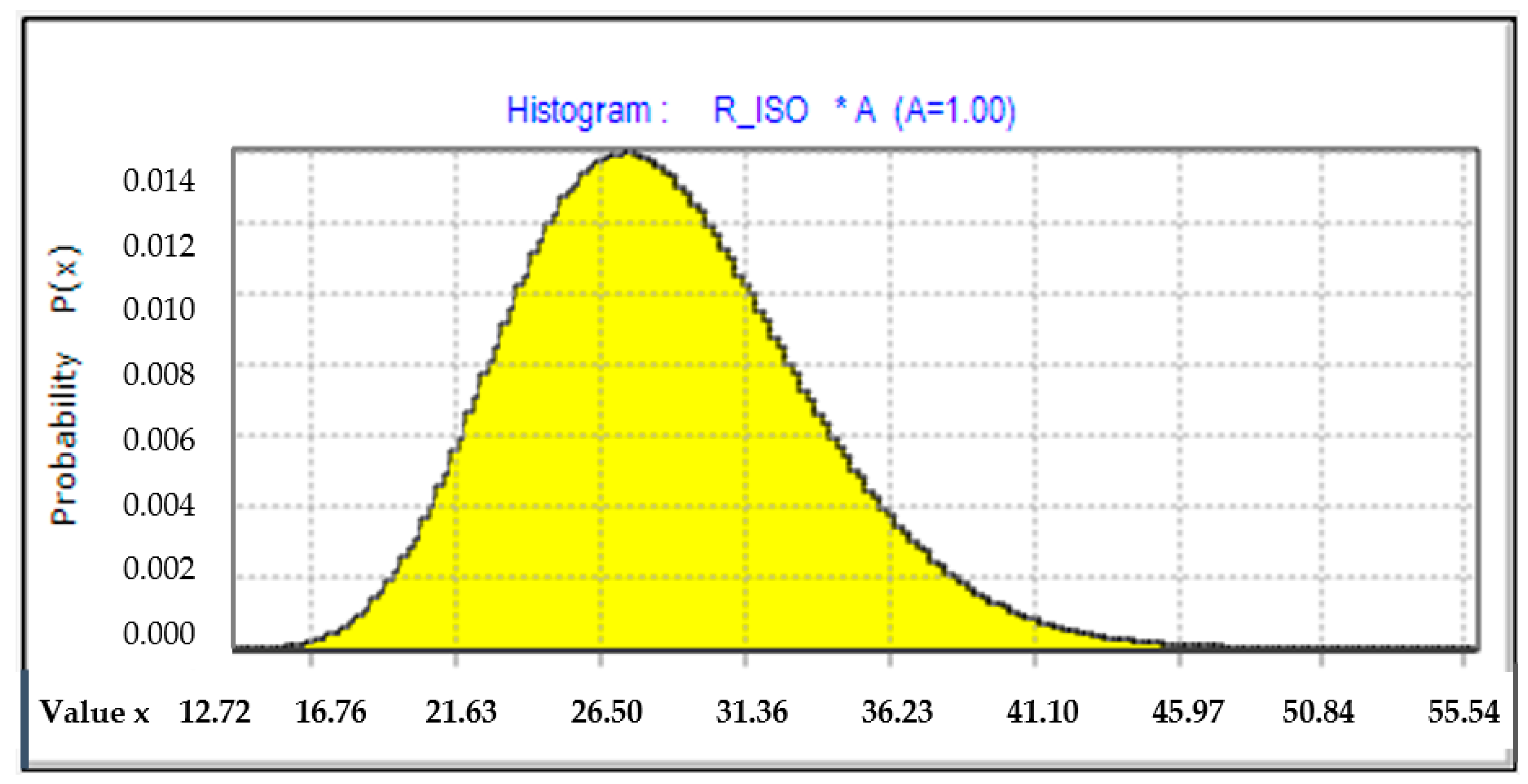
ProbCalc software, a total of five analyses were calculated by probabilistic calculation using the DLL library, which differed in how the input parameters were represented. The first model considers all input parameters to be random variables, while in the other models, only one of the input parameters is a variable, and the others are fixed to the value of their mean. The resulting characteristics of the calculated probability densities of the corrosion rate obtained via sensitivity analysis after 1 year of exposition are provided in
Table 3.
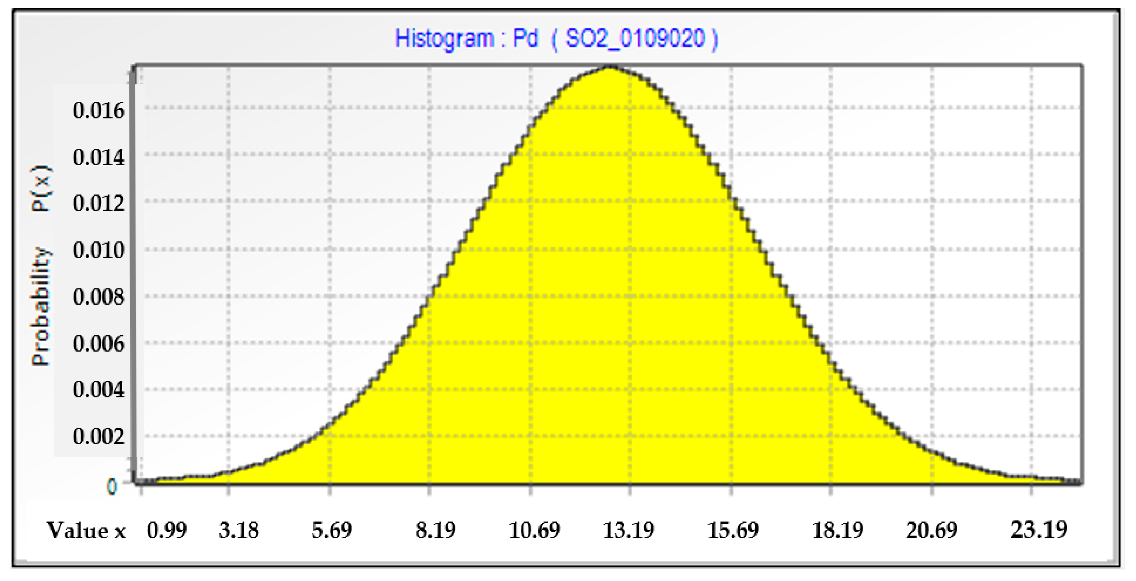
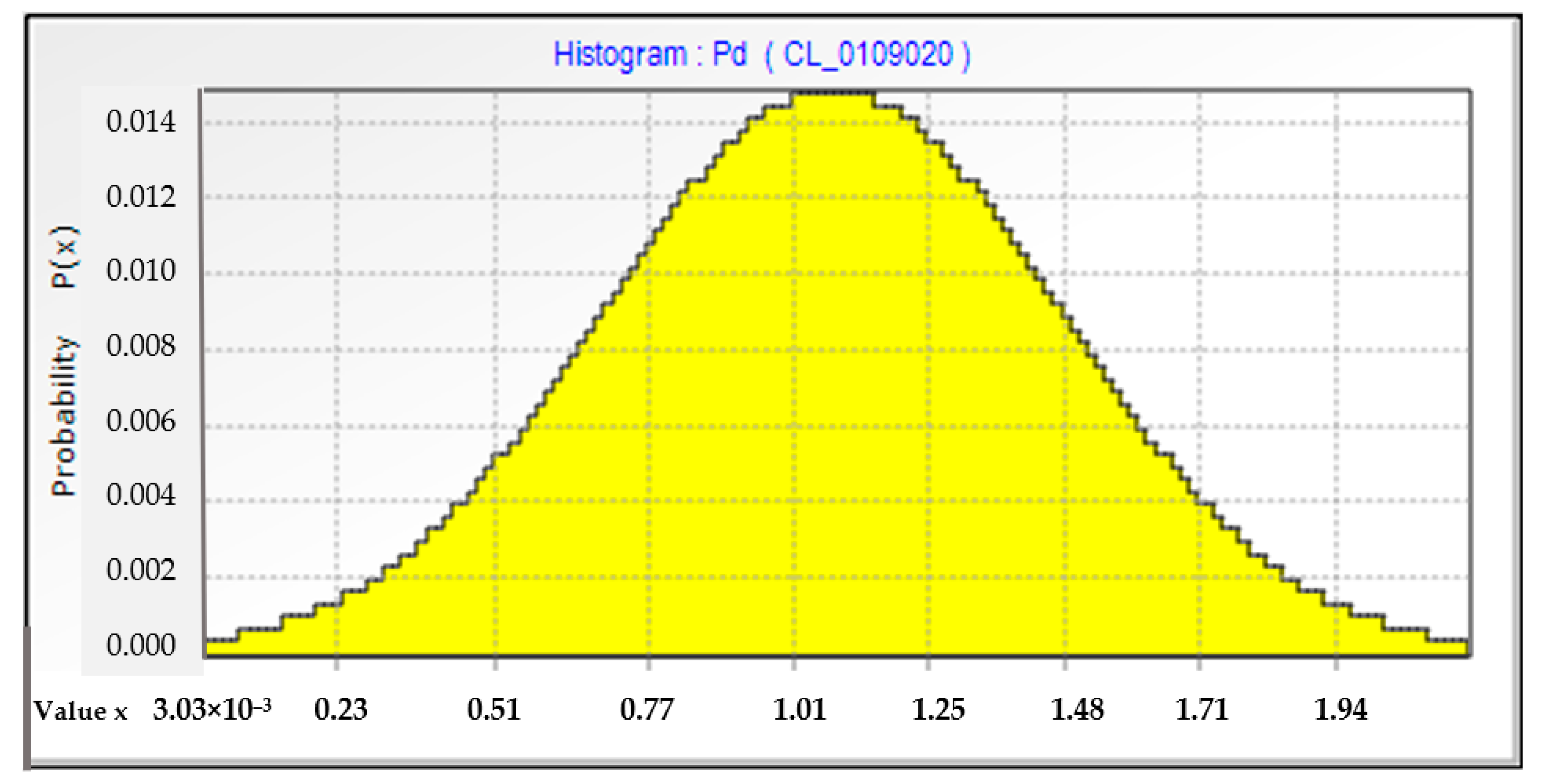
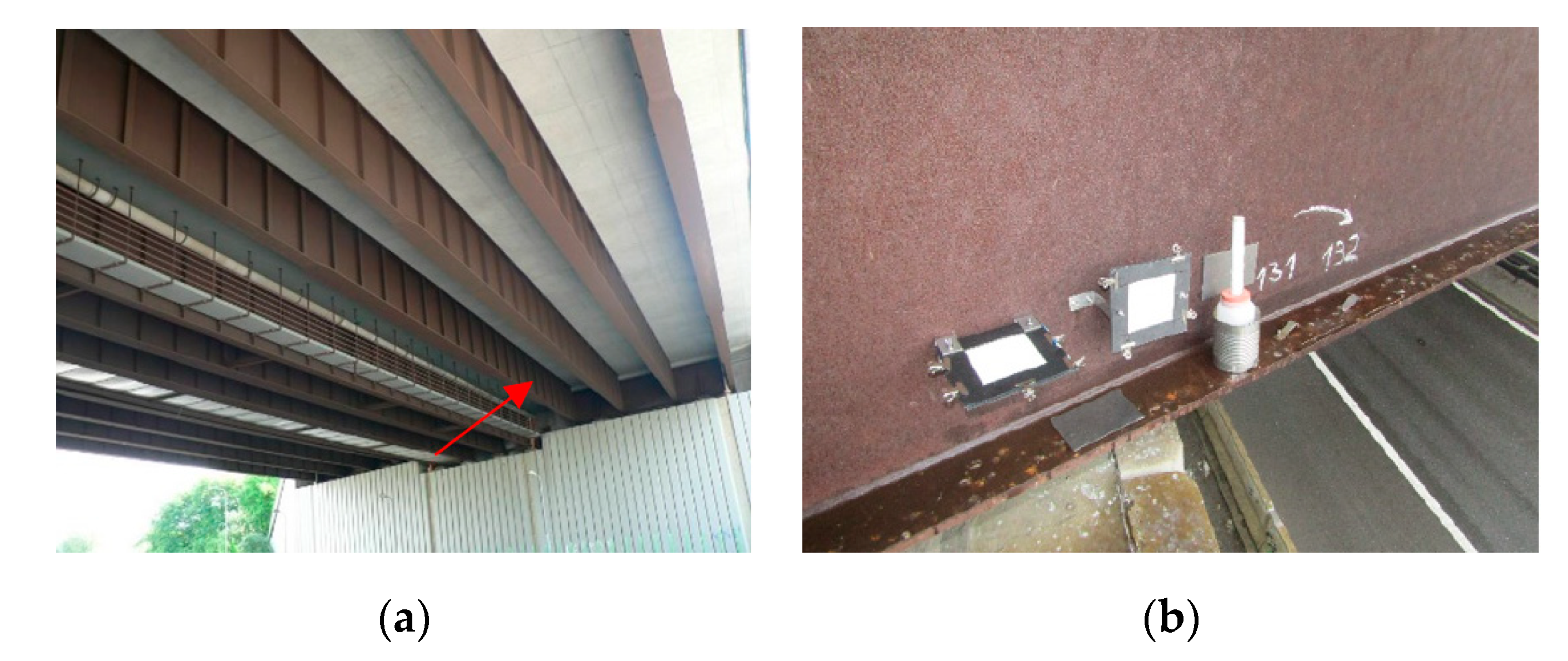
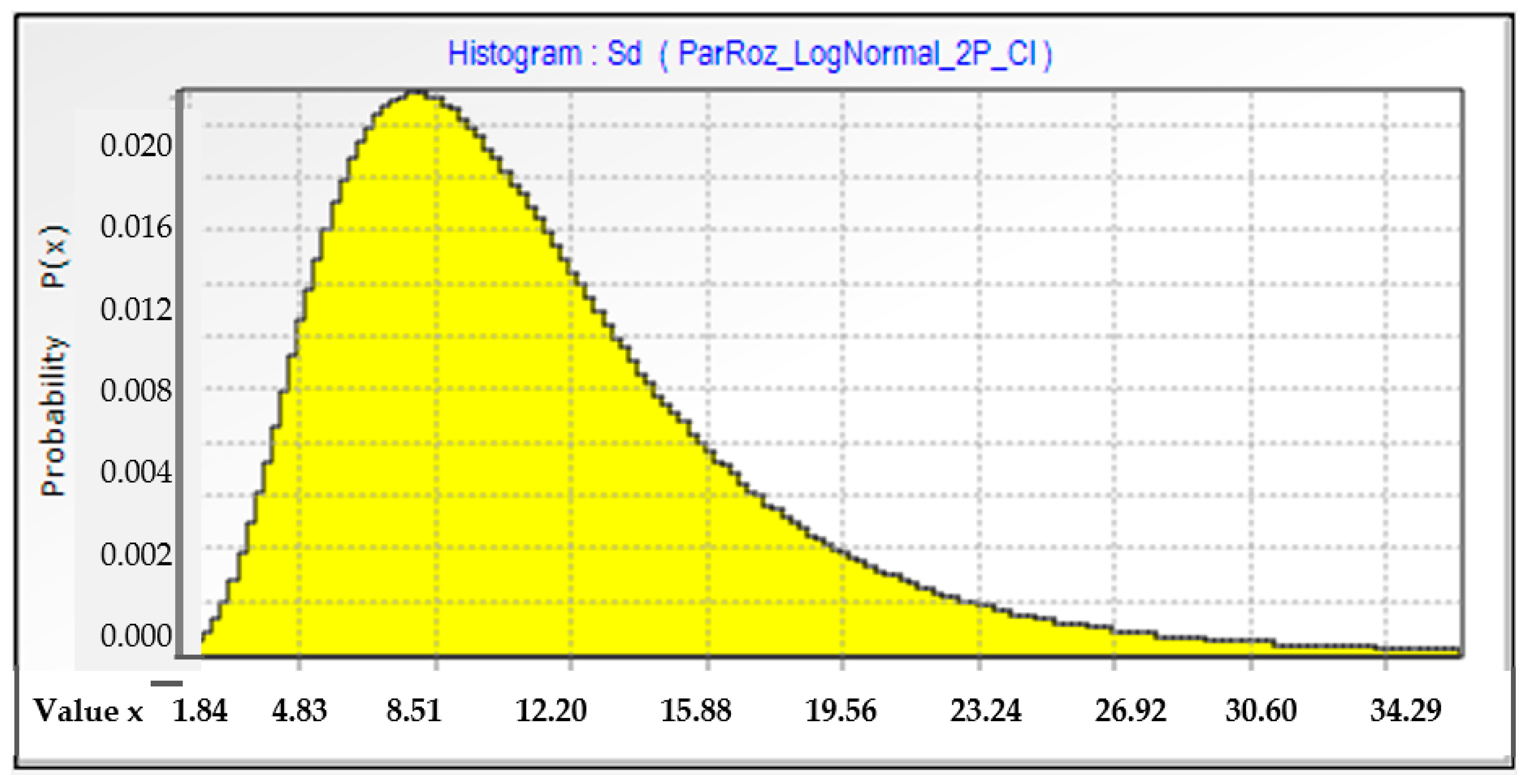
However, at the Kopisty side, the deposition rate of airborne chlorides was very low. In order to evaluate the increased effect of chlorides on the resulting value of corrosion losses specified after 1 year of exposure as per Equation (4), it is hence necessary to make use of the experimentally identified deposition rates of chlorides measured in the vicinity of roads. For the purposes of this article, data measured on a bridge structure in Ostrava were used. The deposition rate of chlorides was measured under the bridge deck on the abutment using the dry plate and wet candle methods (
Figure 11). Experimentally obtained data were used to create a histogram applied in the probability analysis (
Figure 12). To perform a comparison and evaluate the effect of chlorides, the other parameters entering the sensitivity analysis were kept the same as in the Kopisty site, as in the previous example (see
Table 1). The input parameters for the probability density distribution of environmental parameters are provided in
Table 4.
Results of Sensitivity Analysis
The results of the sensitivity analysis (i.e., the sensitivity factors), taking into account the input parameters from
Table 1, are provided on
Figure 13. Among the environmental parameters obtained via long-term measurements at the Kopisty site, the one with the greatest impact on the corrosion rate after 1 year of exposure was the deposition rate of sulfur dioxide SO
2 (
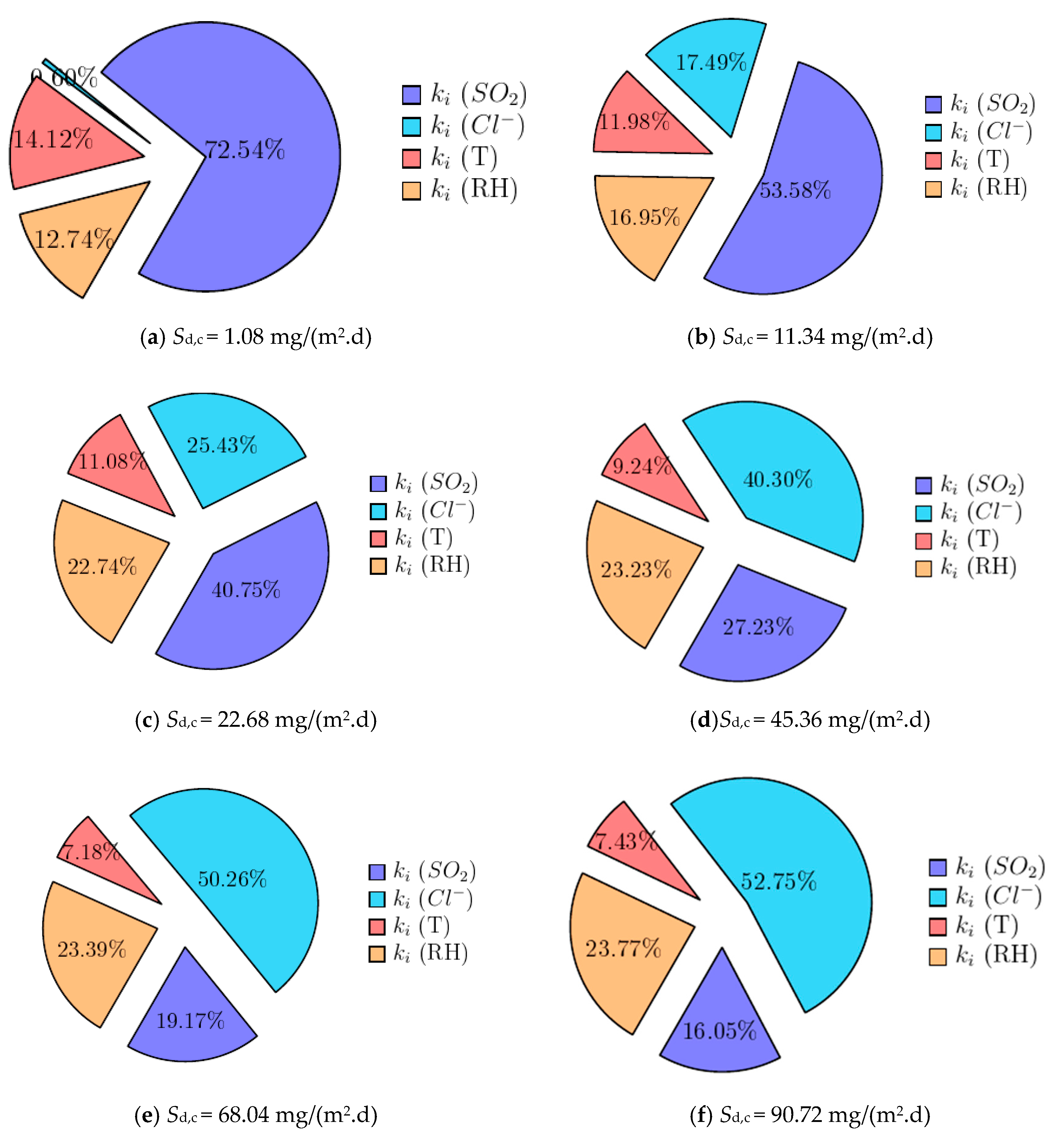
Figure 13a). On the other hand, the smallest impact was associated with the deposition rate of chlorides; indeed, the deposition rate of chlorides was very low at the Kopisty site (the atmospheric station was not located in an area with intensive road traffic).
The effect of chlorides was significant when the sensitivity analysis takes into account the value of the deposition rate of chlorides that matched the actually measured values on the bridge structure in Ostrava, see
Figure 13b. In particular, the sensitivity factor grew from a negligible 0.7 to 17.5%.
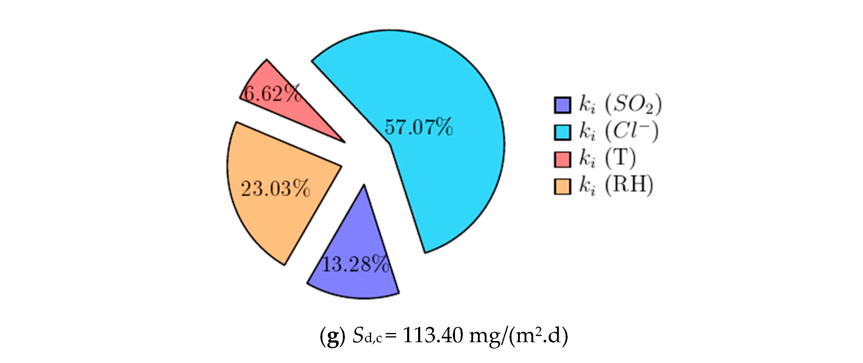
The value of experimentally identified annual average deposition rate of chlorides in Ostrava, however, does not reach values that would have a completely dominant impact on the resulting corrosion rate after 1 year of exposure for the given combination of climatic parameters. Due to the fact of this, a sensitivity analysis was also carried out for two to ten times the annual average deposition rates of chlorides measured on the bridge structure in Ostrava. The dose–response function listed in EN ISO 9223 was derived under the assumption of the average annual deposition rate of chlorides being between 0.4 and 760.5 mg/(m
2.d). Ten times the experimentally determined deposition rate of chlorides at the bridge in Ostrava, amounting to
Sd,c = 113.40 mg/(m
2.d), is still significantly below the upper limit of the values used to derive the dose–response function [
12]. That is why sensitivity analysis was also applied to higher values of chloride deposition (with a maximum corresponding to ten times the measured deposition rate), which all remained in the range of validity of the dose–response function (4).
Sensitivity analysis was carried out for the prediction model as per Equation (4) listed under EN ISO 9223, which is the only one out of the considered equations to consider the direct impact of chlorides. The impact of chlorides is also taken into account in Equation (6), but there, it is derived by converting from the experimental program and by using the relationship between the average annual deposition rate
PM10,dep and the annual average concentration
PM10 in the air. Based on the sensitivity analysis, the deposition rate of sulfur dioxide had the greatest impact on the corrosion rate. However, if the higher deposition rate of chlorides corresponding to the values measured in the vicinity of bridge structures were to be included in the formula, the impact of sulfur dioxide would be lower, and the impact of chlorides would be larger. A higher deposition of chlorides also leads to a higher impact of relative air humidity. The values obtained from the sensitivity analysis for the individual considered average deposition rates of chlorides (amounting to two to ten times the values determined in the experimental measurements in Ostrava) are provided in
Table 5 (where
Sd is the annual average deposition rate of chlorides;
ki-
Sd is the sensitivity factor for the deposition rate of chlorides;
ki-
Pd is the sensitivity factor for sulfur dioxide;
ki-
RH is the sensitivity factor for relative humidity, and
ki-
T is the sensitivity factor for temperature).
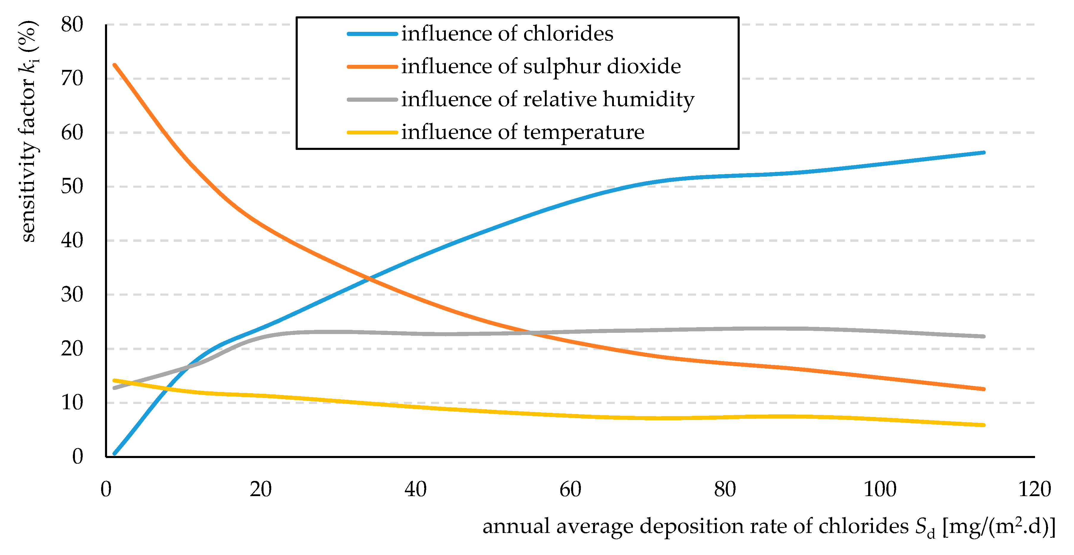
Easier-to-navigate results can be obtained by graphically displaying the values of the sensitivity factor
ki for individual investigated parameters depending on the size of the average annual deposition rate of chlorides (
Figure 14).
Figure 14 clearly shows that as the average annual deposition rate of chlorides grows, so does its impact on the resulting value of the predicted corrosion loss as per Equation (4). This increased impact of chlorides can be expected primarily in microclimates near bridge structures. The impact of relative humidity also exhibited a slight growing trend. The impact of temperature on the resulting corrosion rate did not exhibit significant changes. It is important to note that the sensitivity analysis was carried out for the concrete combination of climatic parameters at the Kopisty site, and other combinations may lead to different ratios of the individual factors.
4. Conclusions
The significant findings in this manuscript can be summarized in the following points:
▪ Environmental parameters affecting corrosion processes are random variables. It is, therefore, advantageous to use a probabilistic approach to predict corrosion damage;
▪ To accurately predict corrosion damage, it is necessary to analyze the measured data from a sufficiently long period. Stochastic models should reflect the observed time trends;
▪ Corrosion damage to steel structures in the vicinity of roads is significantly affected by the deposition rate of chlorides [
10,
11,
26,
27]. Using a stochastic approach, the effect of chloride deposition can be effectively evaluated;
▪ Dose–response functions given in EN ISO 9223 can be used to predict corrosion rates using a probabilistic approach.
Environmental parameters, which affect the corrosion processes on the surface of a metal, are random variables. It is, hence, not possible to predict the specific value of the corrosion rate unambiguously and deterministically for a selected site. The stochastic approach is better suited for such predictions, since it respects the natural variability of the environmental parameters. Statistical methods can be used to introduce development trends of individual random variables over time into prediction models. The use of the probabilistic approach also allows the performance of sensitivity analyses [
33,
34], which can be used to evaluate the impact of individual random variables on the corrosion rate after 1 year of exposure.
The prediction of annual corrosion losses based on probabilistic methods can be carried out via suitable dose–response functions [
14,
15,
16]. Based on the analysis carried out in this article, the formula listed in EN ISO 9223 and the formula obtained from the extensive experimental Multi-Assess program seem to be the best suited for the prediction [
21].
Sensitivity analysis demonstrated that the highest impact on the resulting corrosion rate after 1 year of exposure is caused by the deposition rate of sulfur dioxide. This finding is, however, only valid for sites that are not affected by intense road traffic. When the prediction models were enhanced with data capturing the actual deposition rates of chlorides in the vicinity of roads, the effect of sulfur dioxide dropped, while the effect of chlorides together with that of relative air humidity grew.
Structural engineers are obliged to design reliable structures that can fulfil their roles for the whole duration of their planned service life. Accurate prediction of corrosion aggressiveness of the environment near roads is one of the major inputs for the design of a suitable system of corrosion protection and for planning adequate maintenance and repair systems. Ensuring the long-term sustainability of newly designed as well as previously completed construction projects within the area of transport infrastructure brings significant economic as well as environmental benefits.


