Abstract
Synthetic well log generation using artificial intelligence tools is a robust solution for situations in which logging data are not available or are partially lost. Formation bulk density (RHOB) logging data greatly assist in identifying downhole formations. These data are measured in the field while drilling by using a density log tool in the form of either a logging while drilling (LWD) technique or (more often) by wireline logging after the formations are drilled. This is due to operational limitations during the drilling process. Therefore, the objective of this study was to develop a predictive tool for estimating RHOB while drilling using an adaptive network-based fuzzy interference system (ANFIS), functional network (FN), and support vector machine (SVM). The proposed model uses the mechanical drilling constraints as feeding input parameters, and the conventional RHOB log data as an output parameter. These mechanical drilling parameters are usually measured while drilling, and their responses vary with different formations. A dataset of 2400 actual datapoints, obtained from a horizontal well in the Middle East, were used to build the proposed models. The obtained dataset was divided into a 70/30 ratio for model training and testing, respectively. The optimized ANFIS-based model outperformed the FN- and SVM-based models with a correlation coefficient (R) of 0.93, and average absolute percentage error (AAPE) of 0.81% between the predicted and measured RHOB values. These results demonstrate the reliability of the developed ANFIS model for predicting RHOB while drilling, based on the mechanical drilling parameters. Subsequently, the ANFIS-based model was validated using unseen data from another well within the same field. The validation process yielded an AAPE of 0.97% between the predicted and actual RHOB values, which confirmed the robustness of the developed model as an effective predictive tool for RHOB.
1. Introduction
Formation density is considered one of the main factors in identifying the nature of subterranean formations [1]. It is categorized as a porosity log, which indicates the electron density of the drilled formation [2]. It can be used to provide valuable information to geologists and geoscientists, such as identification of the drilled formations, detection of the evaporite minerals existing within such formations [2], recognition of highly-pressurized formations, identification of the fluid contents of drilled formations [3], investigation of invasion zones for drilled formations [4], assistance with developing geomechanical models that provide information on the mechanical properties of formations [5], and evaluation of the porosity of reservoirs [6].
The density logging tool was first presented in the petroleum industry in the 1960s. It can most simply be described as a nuclear tool that uses a radioactive source to emit gamma rays through formations at a medium level of energy. It then detects and collects the gamma rays reflected from the formations [7]. The radioactive source and detector are lowered into and combined within a drilled well opposite the selected formation. Next, gamma rays are emitted from the radioactive source, which thereafter interact with the electrons of the formation, resulting in a scattering of the rays. These scattered rays are then collected using a detector that is placed a certain distance from the source within the logging tool. The number of gamma rays collected by the detector indicate the density of the electrons within the formation, and accordingly, the formation’s bulk density can be calculated [8]. Formation porosity can be derived from these logging data once the rock matrix density and saturating fluid density are known [9]. This is accomplished using the following formula:
where is the formation porosity, is the rock matrix density, is the formation bulk density (RHOB), and is the fluid density. The RHOB can assist in optimizing the drilling operation by improving bit selection, which is dependent on the nature of the formation being drilled. Moreover, it helps to avoid many disruptive problems such as the loss of circulation, kicks, and wellbore instability, by accurately detecting the downhole formations when drilling [10].
There are two possibilities for measuring RHOB onsite, either using: (1) logging while drilling (LWD) tools while drilling, or (2) wireline logging after the hole has been drilled [3]. However, obtaining LWD measurements can be challenging due to the harsh environment in a hole. Often, several corrections are required, increasing operational costs [11]. Therefore, these data are not always available during drilling operations, and it is preferable to run logging tools after drilling the hole to avoid the logging difficulties that can occur while drilling. As a result, RHOB measurements may not be available during a drilling operation, and identifying the drilled formations while drilling can be confusing due to a lack of data. There is another way to identify a drilled formation other than using logging data, which is analyzing the collected cuttings. However, this method has a lag time, so it cannot provide real-time information on drilled formations [12]. Synthetic well log generation has been introduced as an alternative, robust solution for obtaining log data while drilling, even at sites where well log data are partially absent or not available [13].
Real-time RHOB values provide valuable information on the formation being drilled, and are very helpful to geoscientists and petroleum engineers [14]. When combined with cuttings analyses, they help geologists to identify formations with high confidence and reliability in order to overcome the time lag problem. For drilling engineers, drilling optimization is essential in order to avoid many of the critical problems that can interrupt drilling operations. These problems can be circumvented by detecting zones that cause such issues (such as over pressure zones) by recognizing changes in RHOB trends [14,15]. In addition, when drilling horizontal sections, RHOB can assist in avoiding deviations into the surrounding formations and from the designed path. This is accomplished by tracking the RHOB values that indicate the types of formations being drilled. Furthermore, even when logging measurements are available, another tool for predicting RHOB can be used as a reference to solve the problem of missing data or poor response points within the log, filling in the gaps and providing a continuous data profile.
The nature of the subterranean formation significantly affects the drillability of that formation. Each formation has its own characteristics that affect its resistance to drilling. Weight on bit (WOB), torque (T), and rotating speed (RPM) are adjusted depending on the nature of the formation (e.g., soft or hard) [15]. In addition, the nature of the cuttings for each formation is a key parameter for adjusting standpipe pressure (SPP) to control hole cleaning. All of the aforementioned parameters (in addition to the formation type) play a main role in controlling rate of penetration (ROP) [16,17]. Therefore, these drilling parameters are somehow related to the nature of the drilled formation and, in turn, its density. The usual availability of the mechanical drilling parameters while drilling raises the idea of using them as inputs to estimate RHOB.
Therefore, the objective of this study was to develop a new approach by building novel models for predicting RHOB while drilling, using artificial intelligence tools such adaptive network-based fuzzy interference systems (ANFIS), functional networks (FN), and support vector machines (SVM) in conjunction with mechanical drilling parameters (i.e., ROP, WOB, T, SPP, and RPM) and conventional well logging data in order to generate synthetic low-cost RHOB log data.
2. Data Analysis and Processing
2.1. Data Description
More than 2400 datapoints were collected from a horizontal well in the Middle East, according to the specifications listed in Table 1. These data involve conventional well logging data for RHOB, in addition to the corresponding drilling parameters (i.e., ROP, WOB, T, RPM, SPP, and GPM). The selected drilling parameters are always measured during drilling operation in real time and are strongly affected by the nature of the formations being drilled. The mechanical parameters are used as inputs to feed the developed models and predict the RHOB as an output.

Table 1.
Specifications of the subject well.
The analysis of the statistical parameters listed in Table 2 for the obtained data showed that they were representative and had a good distribution across a wide range, which would enhance the performance of the prediction process. The ranges of the selected data were as follows: ROP from 5.81 to 65.9 ft/h, WOB from 4.6 to 35.3 kIb, RPM from 58.5 to 135.9, T from 1.03 to 8.02 klb ft, SPP from 2393.7 to 3483.9 PSI, GPM from 195.1 to 305.23, and RHOB from 2.43 to 2.91 g/cm3.
Table 2.
Statistical parameters of the obtained data.
2.2. Relative Importance of the Input(s) to the Output
The relative importance of the output (i.e., RHOB) to each of the individually selected inputs was studied in terms of the correlation coefficient (R). R represents the strength of the putative linear association between the variables in question. It is a dimensionless quantity that takes a value in the range from −1 to +1. A correlation coefficient of zero indicates that no linear relationship exists between the studied two parameters, and a correlation coefficient of −1 or +1 indicates a perfect linear relationship. The stronger the correlation of the relationship, the closer the R values come to ±1. It was determined that the RHOB had R values of 0.5, −0.37, 0.73, 0.14, −0.37, and 0.06 with the ROP, RPM, WOB, T, SPP, and GPM, respectively, as shown in Figure 1. For better prediction efficiency, only the input parameters of the highest R with RHOB were selected to feed the models. The GPM was found to have a very low R of 0.06 with the RHOB, indicating a significantly weaker relationship between them as compared to other parameters. To confirm this point, a cross-plot of the GPM and RHOB can be found in Figure 2, showing that the GPM values were almost the same for the entire RHOB range. Thus, the input parameters selected were ROP, WOB, RPM, T, and SPP.
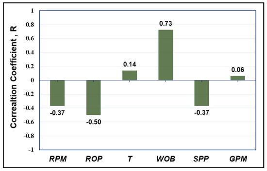
Figure 1.
Input(s)/output relative importance.
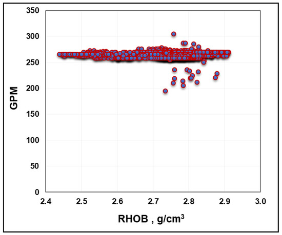
Figure 2.
Cross-plot of GPM (Gallon per minute) vs. RHOB (Bulk density).
2.3. Data Processing
The accuracy of the prediction process relies on the quality of the data used to train the model, so it was very important to filter and analyze the data before building the model [18]. Therefore, the data were filtered for any non-reasonable values (e.g., negative and 999 values). In addition, MATLAB codes were used to remove outliers by applying different statistical methods. Moreover, RHOB log data were analyzed and filtered by tracking the values of the correction data. Reliable RHOB data should have correction values ranging between −0.25 and 0.25 [19]; accordingly, the datapoints with correction values beyond this range were removed. The filtered RHOB well log data used to train the developed models were within the acceptable range of correction, as shown in Figure 3, resulting in greater confidence in the data selected and better prediction results.
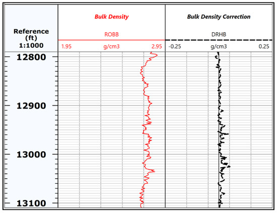
Figure 3.
Sample of the filtered RHOB log data and corresponding correction terms in the log display, with tracks indicating the high quality of the readings.
3. RHOB Model Development
3.1. Adaptive Network-Based Fuzzy Interference Systems (ANFIS)
ANFIS is a supervised learning algorithm that depends on a fuzzy inference system to process data [20]. It is considered an integrated system that combines the concepts of fuzzy logic and neural networks [21]. It was first introduced by Jang [22]. It uses a Takagi–Sugeno inference system that applies conventional Boolean logic (i.e., zeros and ones) [23]. This framework employs a set of fuzzy IF–THEN rules to analyze the system and mimic non-linear relations [20]. It begins by defining the inputs and the required output, and then by specifying fuzzy sets and rules, thereafter training the network to be optimized [21]. Optimization of the number of fuzzy rules is critical for highly accurate predictions, and for avoiding crucial problems such as memorization and overproduction [23]. ANFIS was found to be a reliable predictive tool when applied to petroleum engineering problems [24,25,26,27].
Building the RHOB Model Using ANFIS
After the data were filtered and analyzed, the dataset was then used to build a new model, which employed ANFIS as follows: 1680 datapoints, representing 70% of the total data, were used to train the proposed model, while 720 datapoints (30% of the selected data) were utilized as unseen data to test the developed model’s performance. The obtained data was split randomly using MATLAB during several trials which involved changing the split ratio, in addition to the randomized split data, until it could achieve the best data partitioning scenario which yields the highest accuracy for both training and testing processes. The input data were ROP, RPM, WOB, T, and SPP, which were used to predict the RHOB as the desired output. Grid partitioning (i.e., genfis-1) and subtractive clustering (i.e., genfis-2) were tested to develop the model. It was found that there was some difficulty with obtaining reasonable results when using the Mamdani–Fis type. However, the Sugeno–Fis type yielded much better results. Different cluster radius sizes with various numbers of iterations were tested to optimize the proposed model, as listed in Table 3. The optimization process showed that the Sugeno–Fis type, with a radius of 0.2, yielded the best prediction results. Figure 4a,b shows cross-plots for the predicted and measured RHOB values for training and testing processes, indicating a relatively good match with the R values of 0.95 and 0.93 for the training and testing processes, respectively.
Table 3.
Optimizing the cluster radius for genfis-2 fuzzy logic.
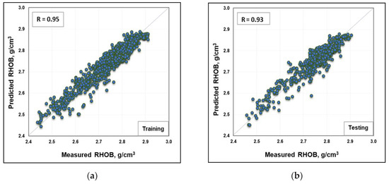
Figure 4.
Cross-plots of the actual and predicted RHOB values using the ANFIS (adaptive neuro-fuzzy inference system)-based model for (a) training and (b) testing processes.
3.2. Functional Networks (FN)
FNs were recently introduced as a powerful predictive tool and a strong competitor with ANN for prediction- and classification-based engineering problems [28,29,30]. They enjoy some privilege among neural networks as they rely on both domain and data knowledge [31]. The functions associated with each neuron use generalized functional models for processing and learning from the data obtained [32]. These functional models are not constant, unlike common sigmodal forms; however, they keep adapting and changing during the learning process, depending on the nature of the dataset used. Thus, since FNs use these multi-argument functional models, they do not need weights to be assigned to the neurons’ connections (unlike neural networks) because the weights’ effects inherently exist within these neuron functions [33,34]. The outputs of the neurons are then forced to converge to an equivalent output [35]. Many applications have been presented in the literature showing that FNs show great promise in the prediction processes for different parameters [36,37].
Building the RHOB Model using an FN
The same dataset was then used to build a new model using an FN. The selected data were divided into a 70/30 ratio, for training and testing the model, respectively. The input data were ROP, RPM, WOB, T, and SPP, which were used to predict the RHOB as the desired output. Five FN techniques were tested: exhaustive search (ES), forward selection (FS), backward elimination (BE), forward–backward (FB), and backward–forward (BF). The performances of the aforementioned methods were compared based on the R and AAPE values to select the optimum method, as listed in Table 4. R is selected to indicate how close the predicted RHOB is to the actual values, while AAPE is used to show the deviation of the predicted RHOB values from the measured values to evaluate the performance of the prediction process. The formulas used for estimating R and AAPE are listed in Appendix A. Based on the results of the optimization process, FB was selected because between the predicted and measured RHOB values, it offered the highest R (0.96) and lowest AAPE (0.95%). Figure 5a,b shows cross-plots of the predicted and measured RHOB values for training and testing processes, indicating a relatively good match between them, with an R of 0.92 and 0.91 for training and testing processes, respectively.
Table 4.
Performance comparison of the Function Network (FN) methods tested.
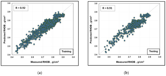
Figure 5.
Cross-plots of the actual and predicted RHOB values using the FN-based model for (a) training and (b) testing processes.
3.3. Support Vector Machines
SVM is a supervised learning tool commonly used for regression, classification, and problems with high degrees of complexity. It is based on the principle of linear classifiers, which enables it to perform classifications depending on the value of a linear combination of features. It is characterized by the ability to transform the data into a higher-degree dimensional space, which provides more space for training examples in the optimum hyperplane [38]. It uses a statistical learning algorithm to minimize generalization errors, rather than decreasing training errors. SVM depends on solving quadratic programming problems with a distinguished, optimized solution [39]. The performance of SVM depends on the tuning process of several parameters that need to be optimized in order to develop the desired predictive model with a high level of accuracy. SVM was recently introduced in the petroleum engineering field and has many applications there [40,41,42,43].
Building the RHOB Model Using SVM
The third model was developed using SVM and applying the same dataset, with 70/30 ratios for training and testing the model. The input data were ROP, RPM, WOB, T, and SPP for predicting the RHOB as the desired output. Two kernel functions were tested to optimize the SVM-based model: gaussian and polynomial functions, with different iterative parameters. The tuning process showed that the gaussian function yielded the best results for R and AAPE. The optimized parameters for the SVM-based model are listed in Table 5. Figure 6a,b shows cross-plots of the predicted and measured RHOB values for training and testing processes, indicating a relatively good match between them, with R values of 0.94 and 0.80 for the training and testing processes, respectively.
Table 5.
Optimized parameters for the SVM (Support vector machine)-based model.
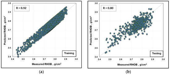
Figure 6.
Cross-plots of the actual and predicted RHOB values using the SVM-based model for: (a) training and (b) testing processes.
A comparison of the results obtained from the three models shows that the ANFIS outperformed the FN and SVM models in predicting the RHOB. It was determined that the R between the predicted and actual RHOB values was 0.95 when using ANFIS, and 0.92 when either FN or SVM were used for the training process. The R value was 0.93 when using ANFIS, and 0.91 and 0.80 when using FN and SVM, respectively, for the testing process. A comparison of the optimized models based on R, AAPE and the mean square error (MSE) can be found in Table 6. Figure 7a–c offers a comparison of the actual and predicted RHOB values using the ANFIS-, FN-, and SVM-based models. Accordingly, the ANN-based model was selected for use in the validation process.
Table 6.
Performance comparison of the optimized methods.
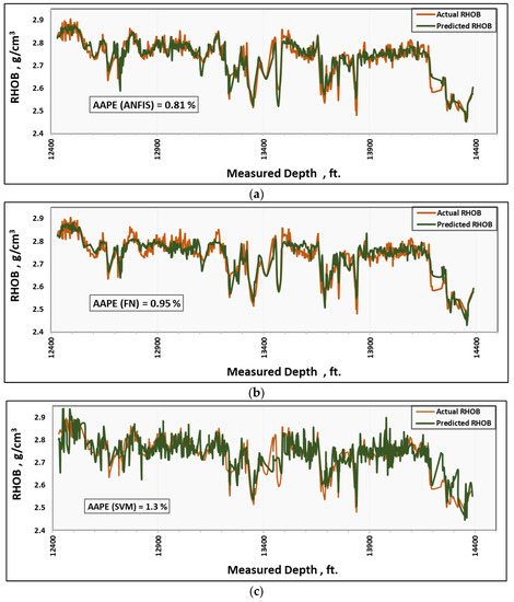
Figure 7.
(a) Comparison of the predicted and actual RHOB values for the testing data using the ANFIS-based model. (b) Comparison of the predicted and actual RHOB values for the testing data using the FN-based model. (c) Comparison of the predicted and actual RHOB values for the testing data using the SVM-based model.
4. Model Validation
The developed ANFIS-based model was validated using field data for another well within the area being examined. The dataset used for the validation process was not employed when building the model. The validation data involved 900 datapoints, including the input parameters (i.e., ROP, WOB, T, SPP, and RPM) and the corresponding RHOB well log data. The prediction results from the ANN model that was developed using these data showed significant agreement with the actual RHOB values, with an AAPE of 0.97%, as shown in Figure 8.
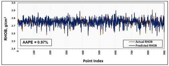
Figure 8.
Significant agreement between the predicted and actual RHOB values using the ANFIS-based model and unseen data during the validation process.
5. Conclusions
In this study, ANFIS, FN, and SVM were used in three models developed to predict RHOB values, based on the following drilling-based mechanical parameter measurements: ROP, WOB, RPM, T, and SPP. Actual measurements (2400 field datapoints from a horizontal well) were used to build the models. The findings of this work can be summarized as follows:
- (1)
- The ANFIS-based model outperformed the FN- and SVM-based models in terms of the accuracy of the RHOB predictions, with an AAPE of 0.81% between the predicted and actual RHOB values, as compared to 0.95% and 1.13% for the FN- and SVM-based models, respectively.
- (2)
- The optimized ANFIS model is capable of predicting RHOB values to a high level of accuracy, as indicated by its R of 0.93 and AAPE of 0.81% between the predicted and measured RHOB values.
- (3)
- The validation process for the ANFIS-based model (using field data from another well) confirmed its outstanding prediction performance, as indicated by an AAPE of 0.97% between the predicted and actual RHOB values.
- (4)
- The developed ANFIS-based model can be used to predict RHOB values with reliably high accuracy, especially in wells where the well logging data are not available or are partially absent.
- (5)
- RHOB predictions that are obtained during drilling using the developed ANFIS-based model will assist in assessing the formations being drilled, and, in turn, avoid interruptions such as kicks and the loss of circulation when identifying the zones causing these issues.
Author Contributions
Conceptualization, S.E., A.A. and S.A.-A.; methodology, A.G. and S.A.-A.; validation, A.G., S.E. and A.A.; formal analysis, A.G. and S.A.-A.; data preparation, S.E. and A.G.; models preparation, A.G., A.A. and S.A.-A.; writing—original draft preparation, A.G.; writing—review and editing, S.E., S.A.-A. and A.A.; visualization, A.Z.A. and S.A.-A.; supervision, S.E. and A.A. All authors have read and agreed to the published version of the manuscript.
Funding
This research received no external funding.
Acknowledgments
The authors wish to acknowledge King Fahd University of Petroleum and Minerals (KFUPM) for making available the various facilities necessary to carrying out this research.
Conflicts of Interest
The authors declare no conflict of interest.
Nomenclature
| AAPE | Average absolute percentage error |
| AI | Artificial Intelligence |
| ANFIS | Adaptive network-based fuzzy interference system |
| BE | Backward elimination |
| BF | Backward–forward |
| ES | Exhaustive search |
| FB | Forward–backward |
| FN | Function network |
| FS | Forward selection |
| MSE | Mean square error |
| R | Correlation coefficient |
| ROP | Rate of penetration |
| RPM | Rotating speed in revolution per minute |
| SPP | Standpipe pressure |
| SVM | Support vector machine |
| T | Torque |
| WOB | Weight on bit |
Appendix A
The formula of correlation coefficient (R), between any two variables (x, y), used in this study is expressed as follows:
Average absolute percentage error (AAPE) is expressed as follows:
where m is the number of points of the dataset.
Mean square error (MSE) is expressed as follows:
where m is the number of points of the dataset.
References
- Ellis, D. Formation porosity estimation from density logs. Petrophysics 2003, 44, 306–316. [Google Scholar]
- Rolon, L.; Mohaghegh, S.D.; Ameri, S.; Gaskari, R.; McDaniel, B. Using artificial neural networks to generate synthetic well logs. J. Nat. Gas Sci. Eng. 2009, 1, 118–133. [Google Scholar] [CrossRef]
- Wraight, P.D.; Evans, M.; Marienbach, E.; Rhein-Knudsen, E.; Best, D. Combination formation density and neutron porosity measurements while drilling. In Proceedings of the SPWLA 30th Annual Logging Symposium, Denver, CO, USA, 11–14 June 1989; Society of Petrophysicists and Well-Log Analysts Inc.: Houston, TX, USA, 1989. [Google Scholar]
- Bassiouni, Z. Theory, Measurement, and Interpretation of Well Logs; SPE Textbook Series; Society of Petroleum Engineers: Houston, TX, USA, 1994; Volume 4, p. 372. [Google Scholar]
- Gatens, J.M.; Harrison, C.W.; Lancaster, D.E.; Guidry, F.K. In-Situ Stress Tests and Acoustic Logs Determine Mechanical Properties and Stress Profiles in the Devonian Shales. SPE Form. Eval. 1990, 5, 248–254. [Google Scholar] [CrossRef]
- Reichel, N.; Evans, M.; Allioli, F.; Mauborgne, M.L.; Nicoletti, L.; Haranger, F.; Laporte, N.; Stoller, C.; Cretoiu, V.; El Hehiawy, E.; et al. Neutron-Gamma Density (NGD): Principles, field test results and log quality control of a radioisotope-free bulk density measurement. In Proceedings of the SPWLA 53rd Annual Logging Symposium, Cartagena, CO, USA, 16–20 June 2012; Society of Petrophysicists and Well-Log Analysts Inc.: Houston, TX, USA, 2012. [Google Scholar]
- Wahl, J.S.; Tittman, J.; Johnstone, C.W. The dual spacing formation density log. J. Pet. Technol. 1964, 16, 1–411. [Google Scholar] [CrossRef]
- Alger, R.P.; Raymer, L.L. Formation Density Log Applications in Liquid-Filled Holes. J. Pet. Technol. 1963, 15, 321–332. [Google Scholar] [CrossRef]
- Spross, R.; Burnett, T.; Freeman, J.; Jones, D.; Paske, W.; Zannoni, S. Formation Density Measurement While Drilling. In Proceedings of the SPWLA 34th Annual Logging Symposium, Calgary, AB, Canada, 13–16 June 1993. [Google Scholar]
- Falconer, I.G.; Burgess, T.M.; Sheppard, M.C. Separating Bit and Lithology Effects from Drilling Mechanics Data. In Proceedings of the SPE/IADC Drilling Conference, Dallas, TX, USA, 28 February–2 March 1988. [Google Scholar] [CrossRef]
- Jackson, C.E.; Heysse, D.R. 1994, Improving Formation Evaluation by Resolving Differences Between LWD and Wireline Log Data. In Proceedings of the SPE Annual Technical Conference and Exhibition, New Orleans, LA, USA, 25–28 September 1994. [Google Scholar] [CrossRef]
- Xu, H.; Li, X.; Li, Y.; Lei, Z.; Sui, S. A Calculation of Cuttings Lag Time for Foam Drilling. Pet. Explor. Dev. 2009, 36, 503–507. [Google Scholar]
- Zhang, D.; Chen, Y.; Meng, J. Synthetic well logs generation via Recurrent Neural Networks. Pet. Explor. Dev. 2018, 45, 598–607. [Google Scholar] [CrossRef]
- Gowida, A.; Elkatatny, S.; Abdulraheem, A. Application of Artificial Neural Network to Predict Formation Bulk Density While Drilling. Petrophysics 2019, 60, 660–674. [Google Scholar] [CrossRef]
- González, J.W.; Valdez, R.; Torres, J.; Medina, F. Identification of Zones of Abnormal Pressures and Determination of the Mechanical Properties of the Rock through Pseudo-Sonic and Pseudo-Density Logs in Conventional and Unconventional Reservoirs. In Proceedings of the SPE Argentina Exploration and Production of Unconventional Resources Symposium, Neuquen, Argentina, 14–16 August 2018. [Google Scholar] [CrossRef]
- Bourgoyne, A.T., Jr.; Millheim, K.K.; Chenevert, M.E.; Young, F.S., Jr. Applied Drilling Engineering; Society of Petroleum Engineers Inc.: Houston, TX, USA, 1986; Volume 2. [Google Scholar]
- Mensa-Wilmot, G.; Calhoun, B.; Perrin, V.P. Formation drillability-definition, quantification and contributions to bit performance evaluation. In Proceedings of the SPE/IADC Middle East Drilling Technology Conference, Abu Dhabi, UAE, 8–10 November 1999; Society of Petroleum Engineers: Houston, TX, USA, 1999. [Google Scholar]
- Hemphill, T.; Bern, P.; Rojas, J.; Ravi, K. Field Validatio of Drillpipe Rotation Effects on Equivalent Circulatin Density. In Proceedings of the SPE Annua Technical Conference and Exhibition, Anaheim, CA, USA, 11–14 November 2007. [Google Scholar] [CrossRef]
- Ellis, D.V.; Singer, J.M. Well Logging for Earth Scientists, 2nd ed.; Springer: Berlin/Heidelberg, Germany, 2007; ISBN 978-1-4020-3738-2. [Google Scholar] [CrossRef]
- Jang, J.S.; Sun, C.T. Neuro-fuzzy modeling and control. Proc. IEEE 1995, 83, 378–406. [Google Scholar] [CrossRef]
- Walia, N.; Singh, H.; Sharma, A. ANFIS: Adaptive neuro fuzzy inference system—A survey. Int. J. Comput. Appl. 2015, 123, 32–38. [Google Scholar] [CrossRef]
- Jang, J.S. ANFIS: Adaptive-network-based fuzzy inference system. IEEE Trans. Syst. Man Cybern. 1993, 23, 665–685. [Google Scholar] [CrossRef]
- Jang, J.S. Input selection for ANFIS learning. In Proceedings of the IEEE 5th International Fuzzy Systems, New Orleans, LA, USA, 11 September 1996; pp. 1493–1499. [Google Scholar]
- Aghli, G.; Moussavi-Harami, R.; Mortazavi, S.; Mohammadian, R. Evaluation of new method for estimation of fracture parameters using conventional petrophysical logs and ANFIS in the carbonate heterogeneous reservoirs. J. Pet. Sci. Eng. 2019, 172, 1092–1102. [Google Scholar] [CrossRef]
- Ja’fari, A.; Kadkhodaie-Ilkhchi, A.; Sharghi, Y.; Ghanavati, K. Fracture density estimation from petrophysical log data using the adaptive neuro-fuzzy inference system. J. Geophys. Eng. 2012, 9, 105–114. [Google Scholar] [CrossRef]
- Ahmed, A.; Elkatatny, S.; Ali, A.; Abdulraheem, A. Comparative analysis of artificial intelligence techniques for formation pressure prediction while drilling. Arab. J. Geosci. 2019, 12, 592. [Google Scholar] [CrossRef]
- Ahmed, A.A.; Elkatatny, S.; Abdulraheem, A.; Mahmoud, M. Application of Artificial Intelligence Techniques in Estimating Oil Recovery Factor for Water Derive Sandy Reservoirs. In Proceedings of the SPE Kuwait Oil & Gas Show and Conference, Kuwait City, Kuwait, 15–18 October 2017; Society of Petroleum Engineers: Houston, TX, USA, 2017. [Google Scholar]
- Castillo, E.; Gutiérrez, J.M.; Hadi, A.S.; Lacruz, B. Some Applications of Functional Networks in Statistics and Engineering. Technometrics 2001, 43, 10–24. [Google Scholar] [CrossRef]
- Anifowose, F.; Labadin, J.; Abdulraheem, A. A least-square-driven functional networks type-2 fuzzy logic hybrid model for efficient petroleum reservoir properties prediction. Neural Comput. Appl. 2013, 23, 179–190. [Google Scholar] [CrossRef]
- Castillo, E.; Cobo, A.; Gutierrez, J.A.; Pruneda, R.E. Functional Networks with Applications: A Neural-Based Paradigm; Springer Science & Business Media: New York, NY, USA, 2012; Volume 473. [Google Scholar]
- Castillo, E.; Hadi, A.S. Functional networks. In Wiley StatsRef: Statistics Reference Online; John Wiley & Sons Inc.: Hoboken, NJ, USA, 2014. [Google Scholar]
- Cobo, A.; Gutierrez, J.M.; Pruneda, E. Functional Networks: A New Network-Based Methodology. Comput. Civ. Infrastruct. Eng. 2000, 15, 90–106. [Google Scholar] [CrossRef]
- Castillo, E.; Cobo, A.; Gutiérrez, J.M.; Pruneda, R.E. Functional Networks with Applications; Springer: Boston, MA, USA, 1999. [Google Scholar] [CrossRef]
- Ahmed, A.; Khalid, M. An intelligent framework for short-term multi-step wind speed forecasting based on Functional Networks. Appl. Energy 2018, 225, 902–911. [Google Scholar] [CrossRef]
- Bello, O.; Asafa, T. A functional networks softsensor for flowing bottomhole pressures and temperatures in multiphase production wells. In Proceedings of the SPE Intelligent Energy Conference & Exhibition, Utrecht, The Netherlands, 1–3 April 2014; Society of Petroleum Engineers: Houston, TX, USA, 2014. [Google Scholar]
- Mahmoud, A.A.A.; Elkatatny, S.; Mahmoud, M.; Abouelresh, M.; Abdulraheem, A.; Ali, A. Determination of the total organic carbon (TOC) based on conventional well logs using artificial neural network. Int. J. Coal Geol. 2017, 179, 72–80. [Google Scholar] [CrossRef]
- Tariq, Z.; Abdulraheem, A.; Mahmoud, M.; Ahmed, A. A Rigorous Data-Driven Approach to Predict Poisson’s Ratio of Carbonate Rocks Using a Functional Network. Petrophysics 2018, 59, 761–777. [Google Scholar]
- Nooruddin, H.A.; Anifowose, F.; Abdulraheem, A. Applying artificial intelligence techniques to develop permeability predictive models using mercury injection capillary-pressure data. In Proceedings of the SPE Saudi Arabia Section Technical Symposium and Exhibition, Al-Khobar, Saudi Arabia, 19–22 May 2013; Society of Petroleum Engineers: Houston, TX, USA, 2013. [Google Scholar]
- El-Sebakhy, E.A.; Hadi, A.S.; Faisal, K.A. Iterative least squares functional networks classifier. IEEE Trans. Neural Netw. 2007, 18, 844–850. [Google Scholar] [CrossRef] [PubMed]
- Anifowose, F.; Labadin, J.; Abdulraheem, A. Improving the prediction of petroleum reservoir characterization with a stacked generalization ensemble model of support vector machines. Appl. Soft Comput. 2015, 26, 483–496. [Google Scholar] [CrossRef]
- Anifowose, F.; Adeniye, S.; Abdulraheem, A.; Al-Shuhail, A. Integrating seismic and log data for improved petroleum reservoir properties estimation using non-linear feature-selection based hybrid computational intelligence models. J. Pet. Sci. Eng. 2016, 145, 230–237. [Google Scholar] [CrossRef]
- Anifowose, F.A.; Labadin, J.; Abdulraheem, A. Ensemble model of non-linear feature selection-based extreme learning machine for improved natural gas reservoir characterization. J. Nat. Gas Sci. Eng. 2015, 26, 1561–1572. [Google Scholar] [CrossRef]
- Tariq, Z.; Mahmoud, M.; Abdulraheem, A. Core log integration: A hybrid intelligent data-driven solution to improve elastic parameter prediction. Neural Comput. Appl. 2019, 31, 1–21. [Google Scholar] [CrossRef]
© 2020 by the authors. Licensee MDPI, Basel, Switzerland. This article is an open access article distributed under the terms and conditions of the Creative Commons Attribution (CC BY) license (http://creativecommons.org/licenses/by/4.0/).