Abstract
Car-sharing plays a positive role in reducing vehicle ownership and greenhouse gas emissions. However, the developmental contradictions between high investment and low revenues hinder the development of the car-sharing industry. Fully understanding car-sharing users can effectively ensure the healthy development of car-sharing companies and promote the development of the entire industry. To this end, this study attempts to develop a user management method that is based on user layering and prediction methods. By using order data from the Lan Zhou car-sharing company in China, this paper develops a clustering method for layering car-sharing users. A multi-layer perceptron model is also developed to categorize these users into different expenditure level categories while considering periodic features. Results show that new users can be divided into three categories according to their expenditures to car-sharing companies within 84 days. After 5 weeks of observation, the 84-day category of new users can be predicted with an accuracy of over 85%. These results provide scientific decision support for the user management and profitability of car-sharing companies.
1. Introduction
By reducing vehicle ownership, car-sharing can contribute to the conservation of resources and alleviation of traffic congestion [1]. In this paper, car-sharing refers to a one-way car-sharing and online time-sharing system mainly supported by mobile technology. A car-sharing company provides resources, such as cars and parking stations, to their users via the Internet. Users can rent a car from a station according to their own travel demands at any time. At the end of their trip, these users need to return their cars to the station and make their payment [2].
Users and companies act as the main participants in car-sharing to ensure the implementation and development of car-sharing travel modes. Car-sharing users can support the normal operation of companies through the consumption of their services. At the same time, companies can improve their service quality to subsequently increase the expenditures of its users. Therefore, mutually reinforcing relationships are formed between user expenditures and company development. However, car-sharing companies face many challenges as the number of their users increases. For example, these companies face the “profit anxiety” problem, which results from their high investment and low revenue during the process of their rapid development. This problem is driven by their inaccurate identification of the revenue contribution level of their users. Accordingly, car-sharing companies have employed an extensive user management strategy where they do not know about their different types of users. Sometimes, companies need to ignore the needs of their high-level revenue contribution users to satisfy the demands of their low-level revenue contribution users. However, losing high-level revenue contribution users will seriously damage the economic interests of a company. In this case, car-sharing companies blindly expand their scale of operations without considering the expenditure level of their users, thereby leading to higher costs and jeopardizing their development. Moreover, car-sharing companies lack scientific methods for mining useful information from a large number of order data, thereby preventing them from managing their users properly and concentrating on the core customer market in their allocation of resources. Therefore, the expenditure behavior of car-sharing users must be analyzed and a user management model must be established.
Given that car-sharing users greatly influence the development of car-sharing companies [3], this study aims to improve the revenue of these companies by analyzing their users. The expenditure of users is equal to the revenue of the company, which is considered a clustering indicator in this study. The clustering method is applied to explore the differences among users of different revenue contribution levels. Furthermore, on the basis of different users’ characteristics, this study builds a multi-layer perceptron model that classifies users according to their expenditure levels.
The contributions of this study are as follows. First, this study explores the new users of different revenue contribution to car-sharing companies by using empirical data. After obtaining the expenditure amounts of new users in their first 84 days with car-sharing companies, a clustering method is applied to categorize these users into three groups. The results indicate that 20% of these users’ revenue contribution account for 70% of revenues contributed by all users. Second, a multi-layer perceptron model is built to predict the revenue contribution level of users in their first 84 days by observing their car-sharing usage characteristics during their first 5 weeks. The prediction accuracy of this model can meet the actual application requirements. This predictive model can also help car-sharing companies identify the value types of their users in the early stage, thereby aiding in their development of user management strategies.
This paper starts by reviewing the literature related to the modeling of car-sharing issues. A detailed description of all datasets and an introduction of the adopted methodology is presented in Section 3. A case study of the users of the Lan Zhou car-sharing company is discussed in Section 4. Several general conclusions are outlined in Section 5.
2. Literature Review
Car-sharing has become a prevalent travel mode in recent years due to its contributions in addressing urban traffic problems. Studies on car-sharing can be divided into two streams. On the one hand, several studies have explored the car-sharing market by investigating the travel behavior of its users, whereas on the other hand, some studies have focused on improving the operational efficiency of car-sharing services.
Users are the key factors that must be considered in the development of car-sharing services. Previous studies that have examined this problem from the perspective of car-sharing users have focused on two issues, namely, the willingness of users to use car-sharing services and the behavior characteristics of these users. Several studies have focused on the car-sharing willingness and preferences of users by conducting questionnaire surveys and interviews [4,5,6,7,8,9,10,11,12]. A selection model has been proposed to identify those variables that can significantly influence user willingness, such as family economic conditions, travel expenses, vehicle demands, and personal attributes. Several studies have attempted to analyze the behavior of car-sharing users by using order data [13,14,15,16,17,18,19,20]. The order data of a car-sharing company mainly refer to the actual car rental information of users that are renting cars from this company. Order data include rental time and rental location information, among others. These studies have explored the characteristics of car-sharing users on the basis of their car usage frequency, travel time and travel distance, and their findings have contributed to the present understanding of car-sharing users.
Improving revenue is among the key factors that determine the sustainability of car-sharing services. A sustainable profitability can also help car-sharing companies overcome their profit anxiety. Previous studies have mainly focused on increasing the revenue of companies and reducing their operational costs. For instance, Shaheen et al. [21] analyzed the global car-sharing market, specifically their parking costs, vehicle models, energy costs, and technologies, and proposed a car-sharing business model for different operating environments with an aim to improve the operational efficiency of car-sharing companies. Alvina et al. [22] studied the multi-parking vehicle allocation problem in the car-sharing operation process and built a car-sharing operation decision model on the basis of three-stage optimization theory. Susan et al. [23] proposed a corresponding commercial operation method for the actual traffic status and user travel characteristics in Beijing and proposed some suggestions for car-sharing operators in the city. Ji et al. [24] identified the operational service capabilities, level of platform design, and convenience of car-sharing facilities as the man factors that affect the development of car-sharing companies and then proposed business strategies in consideration of these factors. Sun et al. [25] constructed a user reservation allocation model with operator profit maximization as its optimization goal. Kong et al. [26] developed a car-sharing dynamic pricing scheme with the goal of maximizing the daily revenue of car-sharing operating systems.
Car-sharing is increasingly becoming a mature industry. However, studies on car-sharing remain in their infancy. Some deficiencies can also be observed in the breadth and depth of extant research. The main deficiencies in the existing literature and the improvements that this research aims to contribute to are summarized as follows. First, previous studies have mainly focused on the willingness of users to use car-sharing services but very few have considered the revenue of car-sharing companies in their investigation. To fill this gap, this study investigates car-sharing services from the perspective of car-sharing companies. Specifically, the findings of this research can provide some references for car-sharing companies to manage their user-centric services. Second, previous studies have mainly focused on the operational efficiency of car-sharing companies but only few have explored the management of car-sharing users with an aim to facilitate the development of car-sharing companies. In the field of economics, those users with a higher expenditure are perceived to be more valuable to companies. Customer value has direct effects on the scale of development of companies because these customers act as the sources of revenue for these companies. In other words, valuable users bring a considerable amount of revenue to companies. Therefore, the differences among users of different revenue contribution levels must be investigated.
3. Data Description and Methodology
3.1. Data Description
3.1.1. Data Collection
The data used in this study are collected from the Lan Zhou car-sharing company. The collected datasets include order data from 1 January 2018 to 31 November 2018 and new user registration data from 1 January 2018 to 31 July 2018. New users are defined as those who have registered with a car-sharing company from 1 January 2018 to 31 July 2018. The order and registration datasets cover different periods because in order to obtain the order data of users within an 84-day time span, the time span of the order dataset should be at least 84 days longer than that of the registration dataset. In this case, the collected datasets can provide the order information of each new user from the time they start using the car to the 84-day time span. This information will be applied in the modeling.
The order dataset also contains information on the car-sharing usage behavior of users during their car-sharing experience. Table 1 presents an example of order data used in this study.

Table 1.
Example of order data.
The user registration data are used to identify the registration characteristics of new users. Table 2 presents an example of registration data used in this research.
Table 2.
Example of registration data.
3.1.2. Data Sampling
In this study, new users are defined as those users who have registered with a car-sharing company from 1 January 2018 to 31 July 2018. This paper attempts to study the car-sharing usage characteristics of new users by classification and prediction. Notably, to realize the modeling, the order data that records the information regarding to the new users within 84 days after starting to use the car are analyzed. The reasons for such selection are as follows:
(1) Reasons for 84-day data selection
The 84-day car usage data of new users are studied because the 84-day behavior of these users can help categorize these users into different types. Short-term car rental users, who use these vehicles for vacation or experiential purposes, have a travel time span of much less than 84 days, whereas long-term car rental users have a car rental time span of more than 84 days. Therefore, using an 84-day duration can help approximate the car rental preferences of uses. Depending on their operational needs, setting a longer duration can help companies understand longer-term user characteristics, but doing so requires longer data time dimensions in modeling. In this study, 84 days can meet the basic needs of the prediction model.
(2) Reasons for new user data selection
The characteristics of new users will be investigated in this study. Car-sharing companies are interested in the revenue contribution types of their new users, which they can determine by using the shortest possible observation period. Accurately predicting the revenue contribution type of users can also help car-sharing companies implement accurate marketing strategies for their users. Therefore, the data for the first 84 days of a new user are used to develop the prediction model.
3.1.3. Data Preprocessing
The employed dataset contains all order data for all users registered before (old users) and after (new users) 1 January 2018. Screening operations are performed as follows to meet the experimental requirements:
(1) Screen new users
The order data from 1 January 2018 to 31 November 2018 are linked with the registration data from 1 January 2018 to 31 July 2018. The users registered between 1 January 2018 and 31 July 2018 are filtered out from the original data and are placed in an empty dataset labelled dataset 1. This dataset contains the order data information (total of 121,472 data points) of users 84 days after they have started using car-sharing services.
(2) Calculate the date of new users on the 84th day
The first car usage date of all users in dataset 1 after their registration period is then calculated. Afterward, 84 days is added to the calculation results to obtain the 84-day duration for each user from the date they have started to use car-sharing services.
(3) Screen order information of new users within their first 84 days
The data of new users registered between 1 January 2018 and 31 July 2018 and their car usage information records from their first day of using car-sharing services up to the 84th day are stored in dataset 2. This dataset contains 69,332 data points covering 5202 users and 600 cars and is treated as the final dataset.
Despite differences in the car-sharing usage behavior and order quantity of car-sharing users, their car usage is fixed to 84 days as denoted by K in Figure 1.
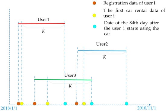
Figure 1.
Data screening.
3.2. Variable Definition
The specific variables defined in this study are shown in the Table 3. The layering variables, namely, the total amount of expenditure and revenue contribution of users, are defined in Section 3.2.1. The total amount of expenditure is used as an indicator to classify car-sharing users, and the results are used as the dependent variable of the prediction model. Section 3.2.2 defines the car-sharing usage behavior variables, which can reflect the car-sharing usage characteristics of users. Some studies have used some of car-sharing usage behavior variables in their analysis, such as average duration, average mileage, time span, car type ratio, and frequency. However, this study introduces new variables, including the heterogeneity of the rental and return stations and the revenue contribution of users. Given that these variables may vary across different users, they are inputted as independent variables into the user prediction model.
Table 3.
Car-sharing usage variable definition.
3.2.1. Layering Variables
(1) Total amount of expenditure
The total amount of expenditure indicates the total amount of money that users have invested in car-sharing companies as shown in Equation (1). The total amount of expenditure of a user is a direct evaluation indicator of his/her contribution to the revenue of a company:
where is the total spending amount of user i in 84 days, and is the amount spent by this user on car-sharing on day.
(2) Revenue contribution
Revenue contribution denotes the ratio of the total amount of revenue contribution of each user to the revenue of a car-sharing company as shown in Equation (2):
where n is the number of users, and indicates that user i contributes to the revenue of a car-sharing company within 84 days.
Revenue refers to the fee paid by a user to a car-sharing company for renting a car, expenses refer to the fuel, vehicle depreciation, and company operating costs shouldered by a car-sharing company in their process of renting out vehicles, and profit is computed as revenues minus expenses. In general, a user of high-level expenditure also has a high revenue contribution to the car-sharing company. Therefore, the total amount of expenditure of a user is a direct evaluation indicator of his/her contribution to the revenue of a car-sharing company. In other words, the total amount of expenditure of a user is a direct source of revenue for a company. High-level revenue contribution users are treated similarly as those users with a high total amount of expenditure. Given that companies can greatly benefit from having many high-level expenditure users, attracting such users has practical significance for company development and growth.
3.2.2. Car-sharing Usage Characteristics
(1) Rental time
Rental time ratio is considered a behavior characteristic of car-sharing users. According to the overall car usage of all users in each time period, a day is divided into seven segments, and the continuous variables are transformed into discrete variables. The time labels and the corresponding real time are shown in Table 4. To contrast the behavior of different users in the same day, the rental time ratio is computed as shown in Equation (3):
where is the ratio of the number of cars used by user i in time period to the number of cars used at all times, is the total number of times that user i uses the car in time period, is the total number of times that user i uses the car on day day, and time is the time period, which value ranges from 0 to 6.
Table 4.
Time and label correspondence table.
(2) Car space
The heterogeneity of rental and return stations denotes the proportion of each user who picks up and returns a car at different stations in 84 days. This variable is computed by using Equation (4):
where is the heterogeneity of rental and return stations, is the number of times that user i picks up and returns a car at different stations on day day, and is the number of times that user i picks up a car on day day.
(3) Car type
A total of five car types are available in the collected dataset. The characteristics of each type are shown in Table 5. The similarities and differences in the car selection preferences of users can be investigated by analyzing these types as shown in Equation (5):
where is the proportion of the total number of times that user i takes car type to that of the total number of times that user i takes all car types, whereas is the number of times that user i takes car type on day day.
Table 5.
Car types and attributes.
(4) Duration and mileage
(1) Average duration and mileage:
where is the average car duration of user i, is the cth car duration of user i, is the total number of times that user i uses the car in 84 days, is the average car mileage of user i, is the cth car mileage of user i, and c is the cth time of user i to rent a car.
(2) Maximum duration and mileage:
where , , , and are the maximum car duration, cth car duration, maximum car mileage, and cth car mileage of user i, respectively.
(3) Minimum duration and mileage:
where is the minimum car duration of user i, and is his/her minimum car mileage.
(5) Frequency characteristics
(1) Time span
Time span refers to the time interval between the last and first car rentals in the first 84 days as shown in Equation (12):
where is the time span of user i, that is, the time difference between his/her last and first car rentals in the first 84 days, refers to the first time that user i uses the car, and refers to the last time that user i uses the car.
(2) Frequency
Frequency refers to the sum of the number of per user within 84 days and is calculated as:
where is the total number of times that user i uses the car in 84 days, and is the number of cars used by user i on day day.
3.3. Layering and Prediction Modeling
Two models are built in this study, namely, a layering model of car-sharing users and a prediction model of users. When analyzing users, they are initially layered before their types are predicted according to their characteristics. Given the complexity of user distribution, classifying these users on the basis of experience alone is sometimes impossible. Therefore, the close relationship between users must be quantitatively determined by using a similarity index or mathematical methods following the principle of the clustering method. This study then establishes a clustering model to layer the users according to their expenditures. Afterward, a classification prediction model is developed given the differences in the car usage characteristics of various types of users. This model can predict the revenue contribution type of new users, thereby helping car-sharing companies understand their users in advance and then formulate a user management strategy.
3.3.1. User Layering Modeling Based on Two-Step Clustering
A car-sharing company can use the expenditure amount of users to maintain its normal operating expenses. Therefore, the expenditure amount of users is of great significance to car-sharing companies. One objective of this paper is to layer users according to their expenditure amount. Layering users can help car-sharing companies learn about their user structure and provide a foundation for their effective operational decision making. Unsupervised classification refers to the classification of data without relying on any classification criteria. Given that the user clustering number is unknown, a two-step clustering method is applied to automatically determine the clustering numbers; this approach can also be used for big data clustering due to its unique data storage solution [27].
The CF tree storage method stores only the sufficient statistics related to the distance calculation in the clustering index rather than the original data itself. In this study, each tree node (group), such as tree node j (group j), stores a sufficient statistic of , where is the number of type j users, is the total amount of expenditures of type j users, is the sum of squares of the total amount of expenditures of type j users, and is the sample size for each category of subtype of type j users and is equal to zero in this study. The sufficient statistic of merge class is for <j, s>, where j and s refer to different types of users. The distance between groups can be easily calculated by using these statistics [28]. Afterward, the likelihood distance of users in each group is calculated by using the sufficient statistic. The CF tree is then established via recursive induction according to the distance between various groups. The tree node generated by the CF tree is then treated as the result of user layering.
3.3.2. Multi-Layer Perceptron Model Considering Periodic Features
The multi-layer perceptron model aims to help car-sharing companies accurately identify the revenue contribution of their users. For these companies, the addition of new users can help them expand their size and increase their revenues. However, when the revenue contribution type of new users is unknown, car-sharing companies are unable to implement a user-centered management strategy.
Car-sharing companies can develop effective operational strategies and maintain high-level revenue contribution users by predicting the expenditure level type of new users during the shortest observation period and by ensuring a high prediction accuracy. To this end, the following prediction time variables are introduced as shown in Figure 2:
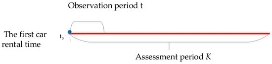
Figure 2.
Schematic diagram of the observation and assessment periods.
Assessment period: Car-sharing companies want to understand the revenue contribution type of their users. This research defines the period from start of use to the future as the assessment period. The expenditure amounts and behavior characteristic of users during the assessment period are unknown. Identifying the revenue contribution level of users during the assessment period in advance can help companies implement differentiated management strategies for their users and rationally allocate their resources. Therefore, the purpose of this research is to identify the type of users during the assessment period in advance by using the prediction model. The duration of the assessment period defined in this paper is denoted by K.
Observation period: The observation period refers to the period when car-sharing companies observe the behavior of its users. In other words, the observation period represents a short period from the first time the user uses a car to the following. The observation period data for each user are fully known, including his/her car-sharing usage behavior and expenditure amount. The assessment period can be predicted by using the characteristics of the user during the observation period. A longer observation period can help companies understand the car-sharing usage behavior of their users and accurately predict their type during the assessment period. However, a longer observation period also introduces a higher time cost, which is not conducive for companies to understand the preferences of their users as soon as possible. Therefore, a shorter observation period is ideal under the premise of satisfying the prediction accuracy threshold. The duration of the observation period defined in this research is denoted by t.
The multi-layer perceptron model can achieve two goals, namely, determine the duration of the observation period and predict the type of new users without a classification label. The shortest observation period is determined by using a specific accuracy threshold. The modeling process is shown in Figure 3.
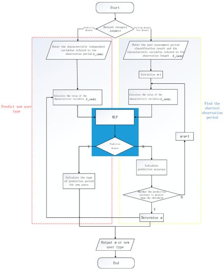
Figure 3.
Prediction process of the multi-layer perceptron model with periodic features.
The key variables in this model are defined as follows. Let denote the individual r belonging to category j, represents a set of type j users, represents the total number of type j users, and represents a set of individual users of all types.
Let denote the ith characteristic variable (including the car usage behavior and static attribute variables) of user r belonging to category j during the observation period duration t. The car usage behavior characteristic variable in this research is related to the duration of the observation period and has nothing to do with the start time of the observation period. The observation period is examined with as the period; therefore, can be expressed as .
Let denote the set of characteristic variables of individual r belonging to category j during the observation period duration , where m is the step size, and n is the number of car-sharing usage behavior characteristics.
Assessment period and observation periods are set for each individual r. Each individual is also given a unique observation period duration, , as shown in Figure 4.
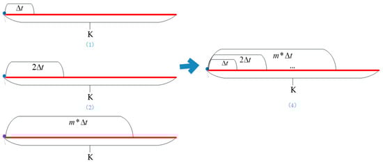
Figure 4.
Sketch of the observation period.
As shown in Figure 5, despite having various starting times, the observation periods of all users have the same duration. The car usage characteristic variable for each user is initially determined, and then the car-sharing usage behavior characteristics in different observation periods are separately examined. The user with the assessment period duration K is then classified and predicted, and the prediction accuracy is eventually determined. This process is described in detail as follows.
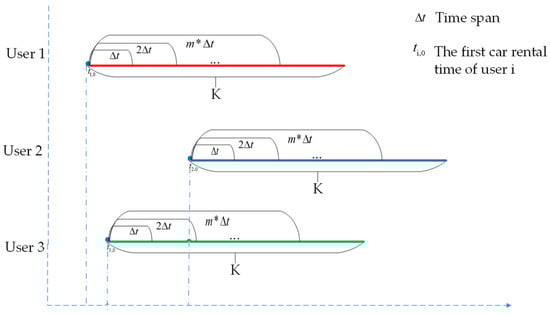
Figure 5.
Schematic diagram of the observation and assessment periods for different users.
First, when the observation period is , the corresponding observation period behavior variable is predicted for the user type during the assessment period within duration K. The prediction accuracy is then obtained. Afterward, when the observation period is , the corresponding observation period behavior variable is predicted for the user type during the assessment period within duration K. The prediction accuracy is then obtained. By analogy, when the observation period is , the corresponding observation period behavior variable is predicted for the user type during the assessment period with duration K. The prediction accuracy is obtained. Find , where is the prediction accuracy threshold, and is the shortest observation period. denotes the prediction accuracy of the observation period by time . Given that the prediction accuracy during a specific period increases along with period and time cost, an acceptable prediction accuracy threshold is pre-set. As the observation period periodically increases, a gap between the prediction accuracy and threshold should be observed. If the prediction accuracy is equal to the threshold, then this accuracy can be satisfied during the observation period. Accepting the prediction accuracy also guarantees the shortest observation period.
4. Case Study
4.1. Layering and Prediction Modeling of Car-sharing Users
4.1.1. Layering Modeling of Car-sharing Users
The two-step clustering of car-sharing users can be divided into the pre-clustering and clustering stages.
(1) Pre-clustering
Step 1: All users and their corresponding expenditure amount are obtained according to the previous calculation. The sufficient statistic is defined in the Section 3.3.1. Then, a CF tree is built, and all user data are entered at the root node. All users are then grouped into a single class, and their sufficient statistics are stored at the root node.
Step 2: The expenditure amount of each car-sharing user is inputted in turn. The distance between the leaf and existing nodes is calculated, and log likelihood distance is used as the similarity judgment index to select the cluster as shown in Equations (14)–(16). The distance threshold is used to determine whether a new node is formed or merged with an existing node. Therefore, the CF tree is established via recursive induction.
where is the likelihood distance of type v users, v = i, j, <j, s>, <i, j> is the joint class of classes i and j, is the total amount of expenditure of type v users, is the number of categorical variables (which is equal to zero in this study because no categorical variables are used in the clustering model), is the number of types under the kth classification, that is, the number of leaf nodes below the k-th node, is the number of type k users, is the estimated variance of the total expenditure amount of type k users, is the estimated variance of the total expenditure amount of type v users in type k, is the information entropy of the total expenditure amount of type v users in type k, is the number of samples of the k-th categorical variable in the l-class in type v, is the number of samples in the v-th category, and d(i,j) is the distance between types i and j.
Step 3: According to the data distribution characteristics, the initial distance threshold is set as 0.01. The distance between the newly read data and the existing leaf node is judged according to the initial threshold and number of leaf node samples. The results are used to determine whether the newly inputted data can be regarded as a new node or merged with an existing node. At this stage, the number of clusters ranges from 2 to 15, thereby suggesting that the maximum number of groups is 15 after this stage. The user data are continuously read until all users are assigned to one leaf node.
(2) Clustering stage
Assume that N groups are obtained at the pre-clustering stage. At the clustering stage, the log likelihood distance between different groups is initially calculated. Afterward, the two closest groups are merged in turn. One large group is eventually obtained after traversing all sample data and looping operations. The Bayesian information criterion (BIC) is used as the basis in this process. If the BIC reaches its minimum value, then the optimal number of clusters is determined. The BIC calculation method is shown in equations (17) and (18):
where J is the category number, N is the number of records in the dataset, is the difference within class j, is the number of classes in class j, is the number of continuous variables, is the number of categorical variables, and is the number of types under the k-th classification, that is, the number of leaf nodes below the k-th node.
4.1.2. Prediction Modeling of Car-sharing Users
(1) Enter the original data
In the case of a fixed assessment period, all training and test sets regarding the characteristic variables and user classification labels are entered. The label does not change during the calculation. The characteristics variables related to the observation period duration are also entered at this stage. The assessment period is set as 84 days, whereas the prediction accuracy threshold is set as 85%. The dependent variable for this study is the user category as shown in Equation (19):
where X is the independent variable, D is the user car usage behavior variable, M is the expenditure amount of users during the observation period, and S is the static attribute variable of users. The independent variables of this prediction model are shown in Table 6. Gender is the only categorical variable in this model. All other continuous variables are normalized.
X = (D, M, S)
Table 6.
Car-sharing user characteristics variables.
(2) Initialization of the observation period value duration
The observation period is set as 7 days, that is, . The car usage behavior variables, total expenditure amount, and user static attribute variables obtained in the previous period after all users start using the car are then calculated. These variables are used as arguments in the user prediction.
(3) Multi-layer perception prediction
The total data after standardization are obtained at the second stage. Among these data, 70% belong to the training set, whereas the remaining 30% belong to the test set. A multi-layer perceptron classification prediction model is also established at this stage, and the training set is used to build a prediction rule between the user category and the user car-sharing usage variable . The test set user data are used to calculate the prediction accuracy.
The user characteristic variable with an observation period of 7 days is inputted into the model. The dependent variable is the user revenue contribution category with an assessment period of 84 days to construct the prediction model. This process is described in detail as follows.
A total of 25 independent variables (23 continuous variables and two dummy variables) for prediction are obtained after processing. Therefore, the input layer of the network has 25 nodes. The neurons between the layers are fully connected. For the output layer, the number of nodes is equal to the number of user categories J. Given that this model is a classification prediction problem, the SoftMax function is selected as the activation function for the output layer. The relative error is selected as the error calculation index [29].
To minimize the model prediction error, the training type selects batch processing, the optimization algorithm determines the synaptic weight, and the conjugate gradient method uses the conjugate gradient algorithm to prevent the local optimal solution. The initial Lambda value of the conjugate gradient method, the initial Sigma is the interval offset. The training termination condition is set to a maximum of 20 steps when the error is not reduced [30].
(4) Prediction accuracy judgment and model output
The multi-layer perceptron prediction model measures the prediction accuracy when the duration of the observation period is and when the assessment period is K. If , then the value of output is treated as the optimal observation period of the model. In other words, the duration should be set for classification prediction. If the assessment period duration is K, then the prediction accuracy reaches .
(5) Cyclic calculation
If m = 1, then the predicted value within the observation period cannot reach the defined prediction accuracy threshold. Therefore, the observation period duration must be increased. In this study, given that m = m + 1, the duration of the existing observation period becomes t = 2Δt. The procedures as presented in the first to the fourth stages are then repeated. The optimal prediction accuracy value for the observation period duration is obtained again, and the m value is obtained until the shortest observation period under the precision threshold condition is obtained.
(6) Rolling forecasts
User management is a dynamic process. The management strategy for each user changes over time depending on the car usage behavior characteristics of users. Therefore, a car-sharing company should use a car usage behavior dataset for its rolling forecasts. In this study, the expenditure level type within 12 weeks can be determined by observing the behavior characteristics of users in the first 5 weeks. First, if the company wants to determine the type of users after 12 weeks, then the company can use the acquired 12-week car usage data to develop the model again. This rolling forecasting method can help the company adjust its operating strategy in time for the changes in the car usage characteristics of its users across different periods. Second, if the company wants to predict the expenditure level type of its users within n years, then the shortest observation period can be calculated by using the developed model. Observing the car usage characteristics of users within the shortest observation period can help predict their expenditure level types within n years. Companies can then dynamically adjust their user management policies.
4.2. Results and Discussion
4.2.1. User Layering Results
Let the cluster number range from 2 to 15 and the optimal one is equal to 3. The first, second, and third categories have 2809, 1367, and 1026 users, respectively. The overall model goodness (average contour factor) is 0.53, thereby suggesting a good performance.
On the basis of the optimal results obtained from the previous clustering experiments, the car-sharing users are classified into three groups according to their total expenditure amount. The results represent the revenue contribution level of users to a car-sharing company. Table 7 shows the optimal clustering results. The percentage of people represents the proportion of various users to the total number of users. The first, second, and third groups account for 19.7%, 26.3%, and 54.0% of all users, respectively. Therefore, the percentage of users from various groups and their total amount of expenditures are not proportional. In this case, each user group is defined according to their contribution to the revenue of car-sharing companies. Despite having the smallest number of users, the first group greatly contributes to the revenue of car-sharing companies (68.9%). Therefore, this group is defined as a high-revenue contribution group (HG). For car-sharing companies, approximately 20% of new users’ revenue contribution accounts for 70% of the revenues contributed by all new users. This conclusion has important implications for car-sharing companies in their development of user-centric operating strategies. Meanwhile, despite having the largest number of users, the third group contributes the least to the revenues of car-sharing companies (9.5%) and is accordingly labeled as the low-revenue contribution group (LG). The second group lies somewhere in between in terms of its revenue contribution and is labeled as the middle-revenue contribution group (MG) accordingly.
Table 7.
User clustering results.
4.2.2. User Prediction Results
A multi-layer perception model that considers periodic features can achieve two purposes in its practical application in car-sharing companies. First, car-sharing companies want to obtain satisfactory predictions with the shortest observation periods. This model obtains the model prediction accuracy value for different observation periods via calculation and comparison. An observation of the prediction accuracy values under different observation periods reveals that the prediction accuracy that satisfies the application requirements can be obtained when the observation period is set as five weeks. Second, the revenue contribution type of new users during the assessment period can be obtained by calculating their behavior characteristics during the observation period.
Table 8 presents the prediction results for the first 6 weeks and the 12th week (the duration of the observation period is equal to the duration of the assessment period). The curve of the prediction accuracy calculated from the 12-week observation period is shown in Figure 6.
Table 8.
Sub-period prediction results.
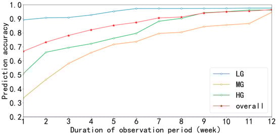
Figure 6.
Twelve-week prediction accuracy distribution.
The prediction accuracy for the 12-week observation period is shown in Figure 6. The prediction accuracy of users gradually increases along with the observation period. Those users with a low revenue contribution obviously have a higher prediction accuracy compared with those with a high revenue contribution. The prediction accuracy of each group is close to 100% at 12 weeks (that is, the observation period is equal to the assessment period) as shown in the figure. Therefore, each characteristic variable has a high fitting precision to the model, thereby proving that the characteristic variable in the predictive model is very scientific and meaningful.
Figure 6 shows that if the prediction accuracy threshold is 80%, the overall prediction accuracy is 82.1%, which exceeds the threshold when the observation period is 4 weeks. In this case, the prediction accuracies of the model for low- and high- revenue contribution users reach 92.7% and 72.2%, respectively. Meanwhile, if the prediction accuracy threshold is 85%, then the overall prediction accuracy is 85.3% which exceeds the threshold when the observation period is 5 weeks. At this time, the prediction accuracies of the model for low- and high- revenue -contributing users reach 95.3% and 76.1%, respectively.
A car-sharing classification prediction model is then built on the basis of user characteristics. This model proves that the revenue contribution type of users three months after using the car can be determined by observing their characteristics over the next five weeks. This model has a prediction accuracy of 85%. However, given the limited amount of data, only the car usage characteristic variables, sex, and age of users are modeled. For car-sharing companies, using additional dimensional data and long-term data observations can extend the assessment period. Therefore, this model has scalability and high practical values.
5. Conclusions
This paper aims to help car-sharing companies alleviate their profit anxiety and to further promote the development of the whole car-sharing industry. To this end, empirical data are used to capture the car-sharing usage characteristics of car-sharing users. By using operating data of the Lan Zhou car-sharing company, the car-sharing users are divided into several groups, which are used as the basis for examining the structure of these users and the efficient operation of car-sharing companies. By using empirical data, the new users can be divided into three groups via clustering analysis. Each group has unique characteristics in terms of their number of users and expenditure levels. Among the new users, 20% generate revenues that account for 70% of the total revenues contributed by all users. Therefore, in the case of limited resources, a car-sharing company can achieve the maximum benefit by analyzing the preferences of this 20% and by rationally configuring its resources. A differentiated management of users can also help retain and increase the satisfaction of high-revenue contribution users, reduce company costs, and increase company revenues.
The revenue contribution type of the 84 days after using a car can be determined by observing their characteristics in the next 5 weeks. This approach has a prediction accuracy of more than 85%. Moreover, the future long-term expenditure level of users can be determined by relying on short-term observations of users. Car-sharing companies should focus on those users with a high revenue contribution, given that increasing the satisfaction of these users can guarantee a source of revenue for these companies. Meanwhile, for those users with a medium revenue contribution, companies must study their demand characteristics and convert them into users with high revenue contribution. Companies who aim to expand their development scale should target those users with a low revenue contribution. Several insights and recommendations for improving the service quality and developing the scale of car-sharing companies are then formulated from the results of the targeted visit investigation.
In sum, a small percentage of high-revenue users can generate revenues that account for the majority of the total revenues of a car-sharing company, whereas other types of users, despite their large number, can only generate minimal revenues for the company. The proposed model has been proven feasible and accurate for predicting the behavior of car-sharing users. These companies must predict their users in advance and manage them scientifically in consideration of their economic benefits. This research has reference significance for car-sharing companies that aim to build a user management system that can help them achieve sustainable development.
Although this study layers the users of car-sharing services, the differences among users from different groups have not been explored. To address this gap, a comparative study of each layer of users will be carried out in the future. Moreover, given the limited amount of data used in this study, a predictive period of 84 days (three months) is considered. In the future, a longer predictive period will be used by collecting additional data. A car-sharing location model will also be developed on the basis of the conclusions obtained from this paper and in consideration of the economic benefits of car-sharing companies.
Author Contributions
Conceptualization and methodology, Q.S. and J.B.; formal analysis, J.B.; validation, J.B.; writing—original draft, Q.S.; writing—review and editing, D.X. and J.B.; supervision, W.G.
Funding
This work is partially supported by the National Natural Science Foundation of China under Grant [No. 71961137008] and National Natural Science Foundation of China [No.71621001].
Conflicts of Interest
The authors declare no conflict of interest.
References
- Genikomsakis, K.N.; Gutierrez, I.A.; Thomas, D.; Ioakimidis, C.S. Simulation and design of fast charging infrastructure for a university-based e-carsharing system. IEEE Trans. Intell. Transp. Syst. 2017, 19, 2923–2932. [Google Scholar] [CrossRef]
- Wappelhorst, S.; Sauer, M.; Hinkeldein, D.; Bocherding, A.; Glaß, T. Potential of electric carsharing in urban and rural areas. Transp. Res. Proced 2014, 4, 374–386. [Google Scholar] [CrossRef]
- Shaheen, S.; Martin, E.W.; Bansal, A. Zero- and Low-Emission Vehicles in U.S. Carsharing Fleets: Impacts of Exposure on Member Perceptions. Bibl. D’Humanisme Renaiss. Trav. Doc. 2015, 118, 741–743. [Google Scholar]
- Mannan, M.S. Car sharing-An (ITS) application for tomorrows mobility. In Proceedings of the 2001 IEEE International Conference on Systems, Man and Cybernetics, e-Systems and e-Man for Cybernetics in Cyberspace (Cat. No. 01CH37236), Tucson, AZ, USA, 7–10 October 2001; Vol. 4, pp. 2487–2492. [Google Scholar]
- Barth, M.; Shaheen, S.A. Shared-use vehicle systems: Framework for Classifying Carsharing, Station Cars, and Combined Approaches. Transp. Res. Rec. 2002, 1791, 105–112. [Google Scholar] [CrossRef]
- Nobis, C. Carsharing as key contribution to multimodal and sustainable mobility behavior: Carsharing in Germany. Transp. Res. Rec. 2006, 1986, 89–97. [Google Scholar] [CrossRef]
- Susan, S.H. Electric Vehicle Carsharing in a Senior Adult Community in the San Francisco Bay Area. Transp. Res. Board 2013, 10, 10–17. [Google Scholar]
- Efthymiou, D.; Antoniou, C.; Waddell, P. Factors affecting the adoption of vehicle sharing systems by young drivers. Transp. Policy 2013, 29, 64–73. [Google Scholar] [CrossRef]
- Fleury, S.; Tom, A.; Jamet, E.; Colas-Maheux, E. What drives corporate carsharing acceptance? A French case study. Transp. Res. Part F: Traffic Psychol. Behav. 2017, 45, 218–227. [Google Scholar] [CrossRef]
- Firnkorn, J.; Müller, M. Free-floating electric carsharing-fleets in smart cities: The Dawning of a Post-Private car Era in Urban Environments? Environ. Sci. Policy 2015, 45, 30–40. [Google Scholar] [CrossRef]
- Zoepf, S.M.; Keith, D.R. User decision-making and technology choices in the US carsharing market. Transp. Policy 2016, 51, 150–157. [Google Scholar] [CrossRef]
- Ju, P.; Zhou, J.; Xu, H.L.; Zhang, J.T. Travelers’ Choice Behavior of Car Sharing Based on Hybrid Choice Model. J. Transp. Syst. Eng. Inf. Technol. 2017, 17, 7–13. [Google Scholar]
- De Luca, S.; Di Pace, R. Modelling users’ behaviour in inter-urban carsharing program: A stated preference approach. Transp. Res. Part A: Policy Pract. 2015, 71, 59–76. [Google Scholar] [CrossRef]
- Morency, C.; Trépanier, M.; Agard, B.; Martin, B.; Quashie, J. Car sharing system: what transaction datasets reveal on users’ behaviors. In Proceedings of the 2007 IEEE Intelligent Transportation Systems Conference, Seattle, WA, USA, 30 September 2007; pp. 284–289. [Google Scholar]
- Müller, J.; Correia, G.; Bogenberger, K. An explanatory model approach for the spatial distribution of free-floating carsharing bookings: A case-study of German cities. Sustain. 2017, 9, 1290. [Google Scholar] [CrossRef]
- De Lorimier, A.; El-Geneidy, A.M. Understanding the factors affecting vehicle usage and availability in carsharing networks: A case study of Communauto carsharing system from Montréal, Canada. Int. J. Sustain. Transp. 2013, 7, 35–51. [Google Scholar] [CrossRef]
- Schmöller, S.; Weikl, S.; Müller, J.; Bogenberger, K. Empirical analysis of free-floating carsharing usage: The Munich and Berlin case. Transp. Res. Part C: Emerg. Technol. 2015, 56, 34–51. [Google Scholar] [CrossRef]
- Kim, J.; Rasouli, S.; Timmermans, H. Expanding scope of hybrid choice models allowing for mixture of social influences and latent attitudes: Application to intended purchase of electric cars. Transp. Res. Part A: Policy Pract. 2014, 69, 71–85. [Google Scholar] [CrossRef]
- Coll, M.H.; Vandersmissen, M.H.; Thériault, M. Modeling spatio-temporal diffusion of carsharing membership in Québec City. J. Transp. Geogr. 2014, 38, 22–37. [Google Scholar] [CrossRef]
- Khan, M.; Machemehl, R. The impact of land-use variables on free-floating carsharing vehicle rental choice and parking duration. In Seeing Cities Through Big Data; Springer: Cham, Switzerland, 2017; pp. 331–347. [Google Scholar]
- Shaheen, S.A.; Martin, E. Demand for carsharing systems in Beijing, China: An exploratory study. Int. J. Sustain. Transp. 2010, 4, 41–55. [Google Scholar] [CrossRef]
- Alvina, G.; Ruey, L.; Meng, Q.; Chan, H. A decision support system for vehicle relocation operations in carshing systems. Transp. Res. 2008, 13, 13–20. [Google Scholar]
- Susan, A.; Elliot, M. Assessing early market potential for carsharing in China: A case study of Beijing. J. Polit. Econ. 2009, 12, 34–45. [Google Scholar]
- Ji, X.; Xian, W. Research on Profitable Mode of carsharing Leasing of Electric Vehicles. Automob. Parts 2015, 50, 39–41. [Google Scholar]
- Sun, H. Research on user reservation allocation optimization model under carsharing mode; Beijing Jiaotong University: Beijing, China, 2016. [Google Scholar]
- Kong, D.; Wang, M.; Ma, D. Research on Dynamic Pricing Strategy of carsharing Leasing of Electric Vehicles. Shanghai Auto 2017, 1, 38–43. [Google Scholar]
- Wang, Z.; Wu, Z.; Tang, Y. Topic detection based on multi-vector and two-step clustering. Comput. Eng. Des. 2012, 33, 3214–3218. [Google Scholar]
- Hu, X.; Cao, Y.; Wu, G. An Effective Data Stream two-step Clustering Algorithm. J. Southwest Jiaotong Univ. 2009, 44, 490–494. [Google Scholar]
- Xie, S.; Girshick, R.; Dollár, P.; Tu, Z.; He, K. Aggregated residual transformations for deep neural networks. In Proceedings of the IEEE Conference on Computer Vision and Pattern Recognition, Honolulu, HI, USA, 21–26 July 2017; pp. 1492–1500. [Google Scholar]
- Bachtiar, L.; Unsworth, C.; Newcomb, R.D. Using multilayer perceptron computation to discover ideal insect olfactory receptor combinations in the mosquito and fruit fly for an efficient electronic nose. Neural Comput. 2015, 27, 171–201. [Google Scholar] [CrossRef] [PubMed]
© 2019 by the authors. Licensee MDPI, Basel, Switzerland. This article is an open access article distributed under the terms and conditions of the Creative Commons Attribution (CC BY) license (http://creativecommons.org/licenses/by/4.0/).