Prediction of Exhaust Emission Costs in Air and Road Transportation

Abstract

In this paper, the calculation of exhaust emission costs originating from aircraft and road vehicles in the base year 2017 and in the forecasting year 2032, in the Republic of Serbia, was carried out. The presented methodology includes a number of influential factors for air transport (airport capacity, number of operations, aircraft type, relevant engine, range) and for road transport (changing of traffic volumes, design and operating speeds, the quality of the pavement structure, type of terrain and category of road sections, dependence of exhaust emission from changes in vehicle speed). It was found that in the current operating conditions, the dominant costs in the total exhaust emission costs are the costs of nitrogen oxides (61%) in road transport, whilst carbon dioxide costs are dominant in air transport (52%). In the future, carbon dioxide costs will have a share of over 80% in the road transport sector and over 58% in the air transport sector in total exhaust emission costs. The average exhaust emission costs per one aircraft operation (international flights) will range from 141 to 145€. In road transport, the average exhaust emission costs at 100 km in 2032 will range from 1.8 to 2.2€.

1. Introduction

Transport is a key driver of economic and social development. Simultaneously, the transport sector is one of the major consumers of energy and consequently one of the major polluters. This sector represents an important source of greenhouse gas (GHG) emissions that are causing global warming and climate change. Also, it contributes to numerous urban and regional pollution-related environmental and human health problems through emissions of various air pollutants. This is also true for the European Union (EU), which makes significant efforts to ensure the reduction of these emissions and environmental sustainability. Namely, according to the European Environment Agency (EEA) data, the transport sector share was 27% of total EU-28 GHG emissions in 2016 [1]. On the other side, although the transport sector, in the last few decades, managed to significantly reduce emissions of air pollutants, such as carbon monoxide (CO) non-methane volatile organic compounds (NMVOCs), sulphur oxides (SO_x), nitrogen oxides (NO_x), as well as particulate matter (PM) emissions, it continues to be a significant source [2]. However, what is particularly worrying is the fact that the transport sector in almost all countries, even in those that represent top carbon emitter economies, has not yet managed to reduce carbon emissions [3]. This is due to the fact that the transport sector, especially road transport, is still dependent on fossil fuels, which is unsustainable in the long run.

According to the Statistical Office data of the Republic of Serbia, road transport plays a main role in passenger and freight transport in the Republic of Serbia. More precisely, road transport, traditionally, has the largest share in total passenger transport performance, expressed in passenger-kilometres (pkm) [4]. Also, analysing the modal split in freight transport it could be noted that the majority of total tonne-kilometres (tkm) in transport of goods is contributed by road and rail transport modes [4]. On the other side, the role of air transport is becoming increasingly important because it indicates significant growth of the performance especially in pkm travelled [4]. Consequently, road transport is the largest consumer of fuel among the transport sector, while on the other side, the share of air transport fuel consumption has been growing rapidly [5]. At the same time, this means that these two transport modes significantly contribute to the overall GHG and air pollutant emissions in the transport sector as well as in the Republic of Serbia in general. In order to develop an environmentally friendly transport system, a rapid reduction of those two transport modes’ emissions will be required. Estimating current and modelling their future GHG and air pollutant emissions and their costs is the first step in achieving this goal.

The paper is organized as described below. The following section presents a brief literature review of the topic. The third section briefly describes the methodology for calculating exhaust emission costs in road transportation, while the methodology for calculating exhaust emission costs in air transportation is presented in section four. The fifth section presents and discusses the obtained results of the external cost estimations in road and air transportation. At the end, the sixth section presents the most important conclusions of this paper.

2. Literature Review

Analysing the relevant literature, it can be noticed that there are numerous studies dealing with sustainable development of transport. In some of these studies the negative environmental impacts are expressed as values of externalities while external cost values are calculated in others [6,7]. Also, it is noticeable that researchers have used different methodology to determine these values. Therefore, comparison of the obtained results from different studies is not straightforward and must be carefully implemented. López-Martínez et al. [8] pointed to the existence of numerous models used to estimate pollutant emissions of road transportation, which can be divided into two large groups, micro or local and macro scale models. These authors developed a methodology for estimating the fuel consumption and emissions of vehicle fleets in urban environments [8], while, for example, Ivković et al. [9] presented the methodology for estimating GHG emission costs in the road and air transport sector on a macro scale.

Understandably, in order to limit a global temperature increase to 2 °C [10], a significant part of transport studies is focused on carbon dioxide (CO₂) and GHG emissions in general [11,12,13]. However, the problem of ecologically sustainable development of transport is far more complex. It concerns not only emissions of GHG but also emissions of air pollutants, such as CO, NMVOC, unburnt hydrocarbons (HC), NO_x, SO_x or PM, with negative impacts at local and regional levels. Many justify not including air pollutants in analyses by arguing that sources of GHG and these gases are the same. Numerous studies have confirmed that through measures created in order to reduce GHG emissions, the emission of air pollutants will also be reduced [14,15,16,17,18]. However, there are other examples in which this is not the case. For example, Fan et al. [19] noted that the selected transport could have a low GHG but high air pollutant emissions and vice versa. As an example, they compared the emissions of a truck and a ship on a route from Rotterdam to Genoa. Obtained results showed that the truck had lower PM₁₀ and NO_x, but higher CO_2eq and sulphur dioxide (SO₂) emissions compared to the ship [19]. On the other hand, Givoni and Rietveld [20] analysed environmental consequences of two different types of aircraft and found that, evaluated in monetary terms, higher aircraft size and lower frequency generates lower total environmental consequences, but, individually speaking, their results showed that this will produce higher local air pollution but lower climate change impact.

Therefore, in order to create an environmentally sustainable transport, as emphasized by [19], efforts should be made to develop a methodology to measure GHG and air pollutants simultaneously. There are numerous studies focusing on estimating and forecasting the emissions of both GHGs and air pollutants as well as developing different mitigation scenarios, especially related to road transport. For example, Lumbreras et al. [21] developed methodology to compute emission projections from road transport in Spain up to 2020 under five different scenarios, while Chavez-Baeza and Sheinbaum-Pardo [22] constructed three passenger road transport scenarios up to 2028 for the Mexico City Metropolitan Area. On the other hand, Liu et al. [23] constructed one business as usual and three improved scenarios that can lead the transport sector in China to achieve lower CO₂ and air pollutant emissions from 2010 to 2050.

This review identifies some research gaps. First, it is clear that there are numerous approaches that can be taken to estimate GHG and air pollutant emissions originating from transportation, which suggests that this is such a complex issue and that there is no one best way to do it. Second, there is space and a need to develop a methodological approach that will be able to consider both GHG and air pollutant emissions and consequently to determine the external costs of emissions for every single GHG or air pollutant in order to determine the total exhaust emission costs as accurately as possible. At the end, we have found that only a small number of studies dealt with measuring exhaust emissions in transportation in Serbia, while studies that calculate external costs of these emissions are even rarer. However, to the best of our knowledge neither of them dealt with prediction of both GHG and air pollutant emissions costs depending on the realization of development projects in the transport infrastructure.

Focusing on the existing research gaps, in this paper, we dealt with the following: first, how to measure and quantify external costs of GHG and air pollutant emissions in transportation and second, how to predict their future values depending on the realization of development projects in the transport infrastructure. Actually, this paper puts emphasis on road and air transportation and their emissions. The calculation of exhaust emission costs originating from aircraft and road vehicles in the base year 2017 and in the forecasting year 2032 was carried out on the main international airport and on the road network of the Republic of Serbia. Depending on the realization of development projects in the transport infrastructure, the range of total exhaust emission costs related to 2032 was determined.

Estimating current and modelling future transport GHG and air pollutant emissions costs presents the first step towards achieving a sustainable and environmentally friendly transport system. It enables transport policy makers to target emissions reductions, to design, implement and foster more effective policies and measures as well as to foresee consequences of the proposed policies and measures on the future GHG and air pollutant emissions and their costs. Also, the applied methodology identifies gases and pollutants with the largest contribution to these costs and emphasizes the importance of simultaneous assessment of GHG and air pollutants.

3. Methodology for Calculating Exhaust Emission Costs in Road Transportation

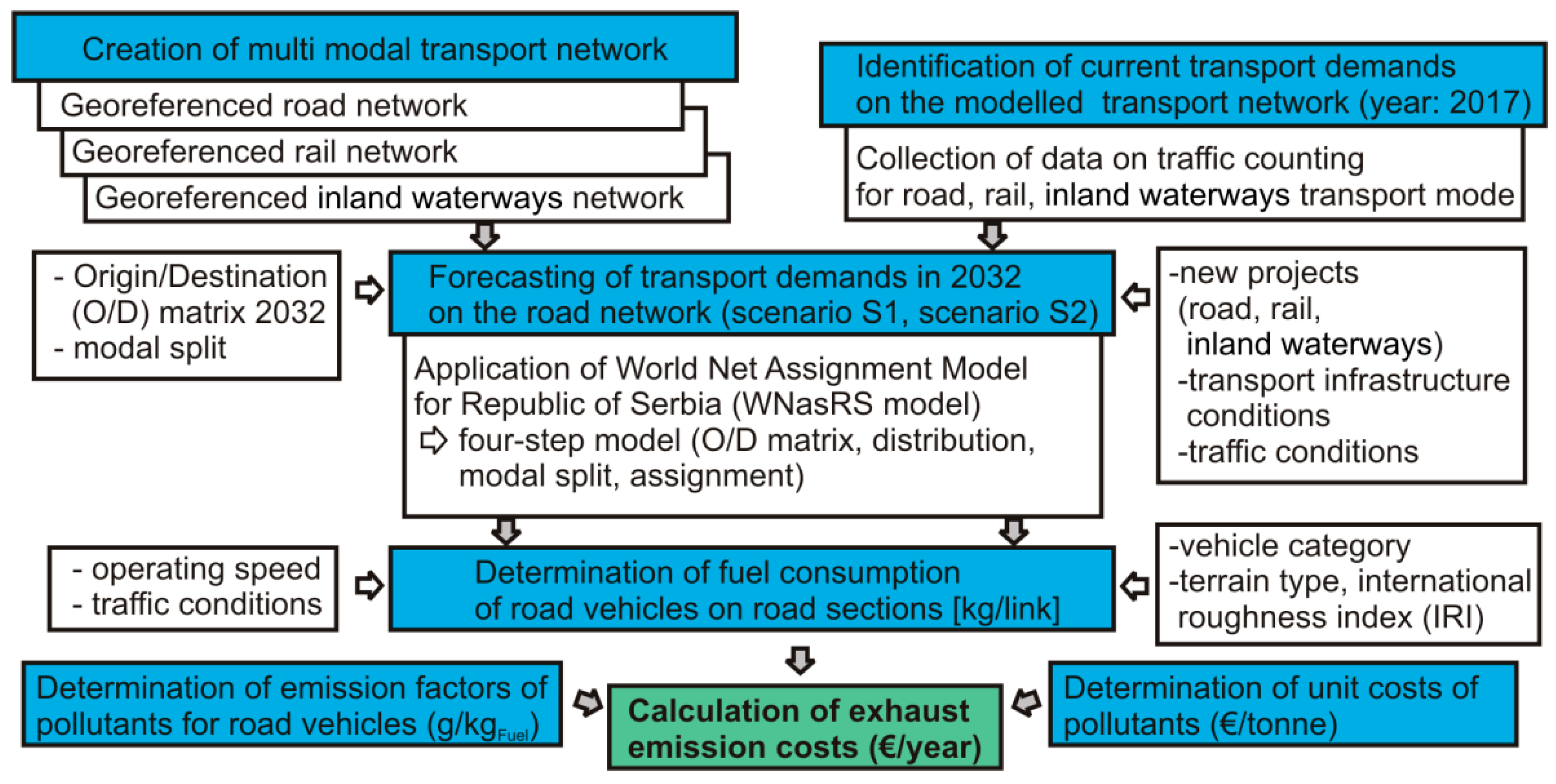
The methodological concept for determining the exhaust emission costs in road transport is shown in Figure 1.

The calculation of exhaust emission costs is carried out for the base year 2017 and forecasting year 2032 in the road network of the Republic of Serbia. For the year 2017 (named scenario S0 (2017)), the required data on the traffic volume were obtained on the basis of traffic counting on the road network for all roads of category IA, IB and part of roads of the category II, according to literature [24,25,26]. Initially, the prediction of exhaust emission costs for 2032 was based on changes in transport demands/volumes and road conditions on the road network. In 2032, two scenarios are considered. The first scenario (named Scenario S1 (2032)) is a scenario without investing in a transport infrastructure with transport demands forecasted in 2032. The second scenario (named Scenario S2 (2032)) is a scenario of maximum investment in the transport infrastructure (with transport demands forecasted in 2032), i.e., on the current multimodal transport network, a total of 27 development projects for road and rail transport mode were implemented, along with several river basin maintenance projects, defined according to the adopted General Master Plan for Transport in Serbia [27]. For the forecast of transport demands in 2032, a classic four-step transport model (first step: trip generation (i.e., creating of an origin/destination (O/D) matrix); second step: trip distribution (i.e., movements (passenger and freight flows) between origins and destinations); third step: modal split (i.e., choice of transport mode for trip realization); fourth step: assignment of traffic flows between origins and destinations by a particular transport mode to a specific route) was used. The model was developed and calibrated during the realisation of the actual national project “Software development and national database for strategic management and development of transportation means and infrastructure in road, rail, air and inland waterways transport using the European transport network models”, No TR36027, 2011–2019 financed by the Ministry of Education, Science and Technological Development of the Republic of Serbia. According to the methodological concept presented on Figure 1, that is, with the defined: traffic demands on the road network, road and traffic conditions on each of the 297 road sections of the road network, fuel consumption of each category of road vehicles, unit costs of pollutants and emission factors, the total exhaust emission costs can be determined by the derived formula, Equation (1):

$${\mathrm{EEC}}_{\mathrm{a},\mathrm{b},\mathrm{c}}={\left({\displaystyle \sum }_{\mathrm{i},\mathrm{j},\mathrm{k}}\mathrm{const}·{\mathrm{DT}}_{\left(\mathrm{i},\mathrm{j}\right)}·{\mathrm{FC}}_{\left(\mathrm{i},\mathrm{j}\right)}·{\mathrm{f}}_{{\mathrm{FC}}_{\left(\mathrm{i},\mathrm{j}\right)}}·{\mathsf{\rho }}_{\mathrm{f}}·{\mathrm{L}}_{\left(\mathrm{j}\right)}·{\mathrm{EF}}_{\left(\mathrm{i},\mathrm{k}\right)}·{\mathrm{f}}_{{\mathrm{EF}}_{\left(\mathrm{i},\mathrm{j},\mathrm{k}\right)}}·{\mathrm{UC}}_{\left(\mathrm{k}\right)}\right)}_{\mathrm{a},\mathrm{b},\mathrm{c}}$$

(1)

where:

• EEC—exhaust emission cost for the road network (€/year);
• DT—annual average daily traffic per vehicle category (vehicle/day);
• FC—fuel consumption of vehicle (l/km);
• f_FC—correction factor of fuel consumption (–);
• ρ_f—density of fuel (ρ_gasoline = 0.710 kg/L, ρ_diesel = 0.835 kg/L, ρ_{liquid petroleum gas} = 0.560 kg/L);
• const—constant (const = 3.65 × 10⁻⁴);
• L—length of road section (km);
• EF—emission factors (g_pollutant/kg_fuel);
• f_EF—factor of change in the emission of pollutants, depending on the different engine mode (i.e., at different vehicle speeds);
• UC—unit cost of pollutant (€/tonne);
• i—index of vehicle category (passenger cars-gasoline, passenger cars-diesel, passenger cars-liquid petroleum gas (LPG), buses, light trucks, medium trucks, heavy trucks, articulated trucks);
• j—index of road section (a total of 297 road sections within the road network);
• k—index of pollutants (CO, NO_x, NMVOC, methane (CH₄), PM, CO₂ and SO_x);
• a—index of Scenario S0 (2017); b—index of Scenario S1 (2032); index c—Scenario S2 (2032).

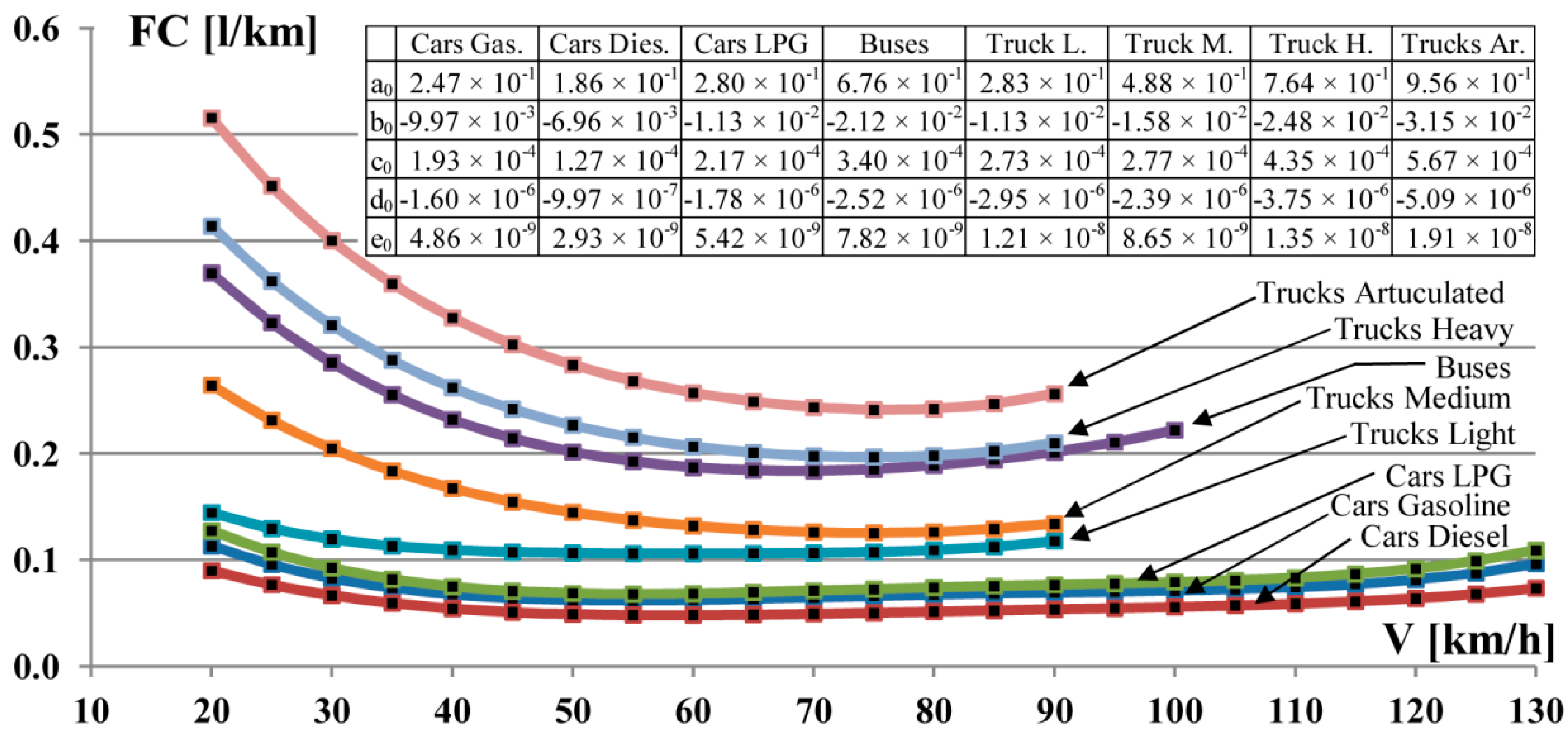
In Equation (1), the FC on the individual road section was obtained by regression analysis of data in the form of “fuel consumption-vehicle operating speed” pairs (“FC-V”). The pairs “FC-V” by vehicle categories were obtained from the Highway Development and Management (HDM) model for a total of nine combinations of terrain type and values of IRI of concrete road section (terrain type: flat, hilly or mountainous; IRI: 2, 5 or 8 m/km). For each road section, it was necessary to collect the data about the IRI and the terrain type. The dependence of fuel consumption on operating speed, on the road section (j) for vehicle category (i), is given in the form of fourth-degree polynomials of Equation (2):

$${\mathrm{FC}}_{\left(\mathrm{i},\mathrm{j}\right)}={\mathrm{a}}_{0_{\left(\mathrm{i},\mathrm{j}\right)}}+{\mathrm{b}}_{0_{\left(\mathrm{i},\mathrm{j}\right)}}·{\mathrm{V}}_{\left(\mathrm{i},\mathrm{j}\right)}+{\mathrm{c}}_{0_{\left(\mathrm{i},\mathrm{j}\right)}}·{\mathrm{V}}_{\left(\mathrm{i},\mathrm{j}\right)}^2+{\mathrm{d}}_{0_{\left(\mathrm{i},\mathrm{j}\right)}}·{\mathrm{V}}_{\left(\mathrm{i},\mathrm{j}\right)}^3+{\mathrm{e}}_{0_{\left(\mathrm{i},\mathrm{j}\right)}}·{\mathrm{V}}_{\left(\mathrm{i},\mathrm{j}\right)}^4$$

(2)

where: a₀, b₀, c₀, d₀, e₀—regression coefficients of vehicles category (i) on the road section (j); V—operating speed of vehicles category (i) on the road section (j).

Figure 2 gives an example of the “FC-V” dependence in the case of the road section with attributes: terrain type = flat and IRI = 2. In Figure 2 the corresponding regression coefficients in the table are shown.

Due to the mutual interaction of vehicles in the traffic flow, the fuel consumption was corrected with the correction factor f_FC. This factor was obtained from the matrix of design and operating speeds taken from [28]. The f_FC values for passenger vehicles range from 1 to 2.5 and from 1 to 1.8 for freight vehicles.

The emission factors from Equation (1), EF_(i,k), represent the referent emission of pollutants (k) per vehicle category (i) that were produced at a specified operating speed. These factors are expressed in grams per kilogram of burned fuel. Since there is no such data for Serbia, EF_(i,k) values for 2017 were obtained as the average values of emission factors for individual vehicle category (i) known for 28 European countries from literature [29]. Bearing in mind the year (2005) for which the values are given in this document, and that the average age of road vehicles in Serbia is about 16 years [30], these values have been adopted as valid referent values of emission factors at the passenger vehicle speed of 70 km/h and freight vehicles speed of 50 km/h (

Table 1. Referent values of emission factors per vehicle categories (g_pollutant/kg_fuel).

	Cars-Gasoline	Cars-Diesel	Cars-LPG	Buses	Trucks-Light	Trucks-Medium	Trucks-Heavy	Trucks-Articulated
CO2017	108.26	4.44	84.70	9.14	8.07	7.38	7.68	8.44
CO2032	30.25	1.23	23.89	6.07	3.31	3.18	5.40	6.18
NOx,2017	11.62	12.51	15.20	35.45	15.49	29.66	33.82	36.83
NOx,2032	2.11	2.61	2.92	2.92	2.94	3.03	3.05	3.11
NMVOC2017	13.46	0.99	13.64	2.67	1.61	1.96	2.10	2.42
NMVOC2032	6.78	0.12	6.56	0.38	0.33	0.34	0.34	0.38
CH4,2017	0.98	0.13	0.32	0.31	0.11	0.19	0.23	0.25
CH4,2032	0.50	0.02	0.15	0.05	0.02	0.03	0.04	0.04
PM2017	0.03	1.38	0.00	1.20	1.78	0.99	1.01	1.13
PM2032	0.01	0.18	0.00	0.22	0.19	0.19	0.19	0.23
CO2,2017	3169	3179	3024	3174	3177	3174	3172	3176
CO2, 2032	3169	3179	3024	3174	3177	3174	3172	3176
SOx,2017	0.01	0.006	0.000	0.006	0.006	0.006	0.006	0.006
SOx,2032	0.002	0.001	0.000	0.001	0.001	0.001	0.001	0.001

).

The estimation of the emission factors for 2032 was made considering the age of road vehicles in 2017 and that the current vehicles on average meet the emission standards between EURO3 and EURO4 (EURO3 was implemented in 1999/2000, while EURO4 was implemented in 2005). Due to the necessary modernization of the vehicle fleet, it is expected that the vehicles for the forecasted year 2032 will be on the EURO6 level on average. Based on the difference in exhaust emissions for vehicles with EURO6 and EURO3/EURO4 engines [31], Table 1 shows the estimated reduced values for CO, NO_x, NMVOC, CH₄ and PM, which are valid for 2032. According to [31], the difference in fuel consumption for vehicles with a EURO6 engine in relation to vehicles with EURO3/EURO4 engines is insignificant. Therefore, for 2032, emission factors for CO₂ are the same as for the base year 2017, since CO₂ emission is directly dependent on fuel consumption [32]. On the basis of the trend of reducing the amount of sulphur in the fuels [29], for 2032, sulphur amounts of 1 mass ppm (1 ppm = 1.00 × 10⁻⁶ g of sulphur/g of fuel) of gasoline and 0.5 mass ppm of diesel were adopted. Emission factors of sulphur oxides was calculated as 2 × 1.00 × 10⁻⁶ × 1000 = 0.002 g_SOx/kg_fuel for gasoline and 2 × 0.50 × 10⁻⁶ × 1000 = 0.001 g_SOx/kg_fuel for diesel [31].

Since the pollutant emissions change with the engine operating mode, the dependence of the change of pollutant emissions in relation to the operating speed was determined. In Equation (1), this change is expressed by the factor f_EF(i,j,k). Based on the analysis of data on the variation of pollutant emission at different vehicle speeds from [31], and by the regression analysis of the dependence between the factor f_EF(i,j,k) and the operating speed, the form of the fourth degree polynomial for pollutants CO, NO_x, NMVOC, CH₄ and PM, was determined using Equation (3):

$${\mathrm{f}}_{{\mathrm{EF}}_{\left(\mathrm{i},\mathrm{j},\mathrm{k}\right)}}={\mathrm{a}}_{1_{\left(\mathrm{i},\mathrm{k}\right)}}+{\mathrm{b}}_{1_{\left(\mathrm{i},\mathrm{k}\right)}}·{\mathrm{V}}_{\left(\mathrm{i},\mathrm{j}\right)}+{\mathrm{c}}_{1_{\left(\mathrm{i},\mathrm{k}\right)}}·{\mathrm{V}}_{\left(\mathrm{i},\mathrm{j}\right)}^2+{\mathrm{d}}_{1_{\left(\mathrm{i},\mathrm{k}\right)}}·{\mathrm{V}}_{\left(\mathrm{i},\mathrm{j}\right)}^3+{\mathrm{e}}_{1_{\left(\mathrm{i},\mathrm{k}\right)}}·{\mathrm{V}}_{\left(\mathrm{i},\mathrm{j}\right)}^4$$

(3)

where: a₁, b₁, c₁, d₁, e₁—regression coefficients of the vehicle category (i) for the pollutant (k).

The values of f_EF(i,j,k) are in the wide range of 0.3 to 4, depending on the vehicle category, different pollutants and operating speed. This factor corrects the referent values of the emission factors (from Table 1) relative to the operating speeds.

The calculation of exhaust emission costs implies the determination of unit costs of pollutants marked with UC_(k) in Equation (1). The unit costs were obtained on the basis of research [33]. According to this document, in the first step, for each of the countries in Europe, the basic unit costs of pollutants NO_x, SO_x, NMVOC and PM in 2000 were determined. At the same time, socio-economic characteristics of countries and geographical position have been considered. Given the estimated average gross domestic product (GDP) growth at the European level of 2% in the period up to 2030 and 1% in the period from 2030 to 2050, it is possible to determine the unit cost of pollutants for any year in the range from 2000 to 2050. Data on unit costs of pollutants for 2017 and 2032 for pollutants NO_x, SO_x, NMVOC and PM are given in

Table 2. Unit costs of pollutants (€/tonne).

	NOx	NMVOC	SOx	PM
2017	10,052.22	563.09	9199.13	25,721.85
2032	12,594.45	700.53	11,581.08	32,570.65

.

According to [34], the unit costs for CO₂ in 2017 and 2032 have been adopted in the amount of 35.5 €/tonne and 58 €/tonne, respectively. Since CH₄ and CO in long distance transport can be treated as pollutants that affect climate change [35], and on the basis of global warming potential (GWP) values for CH₄ and CO (GWP_CH4 = 28; GWP_CO = 3; [36]), the following unit costs were adopted: UC_CH4,2017 = 994 €/tonne, UC_CH4,2032 = 1624 €/tonne, UC_CO,2017 = 106.5 €/tonne, UC_CO,2032 = 174 €/tonne.

4. Methodology for Calculating Exhaust Emission Costs in Air Transportation

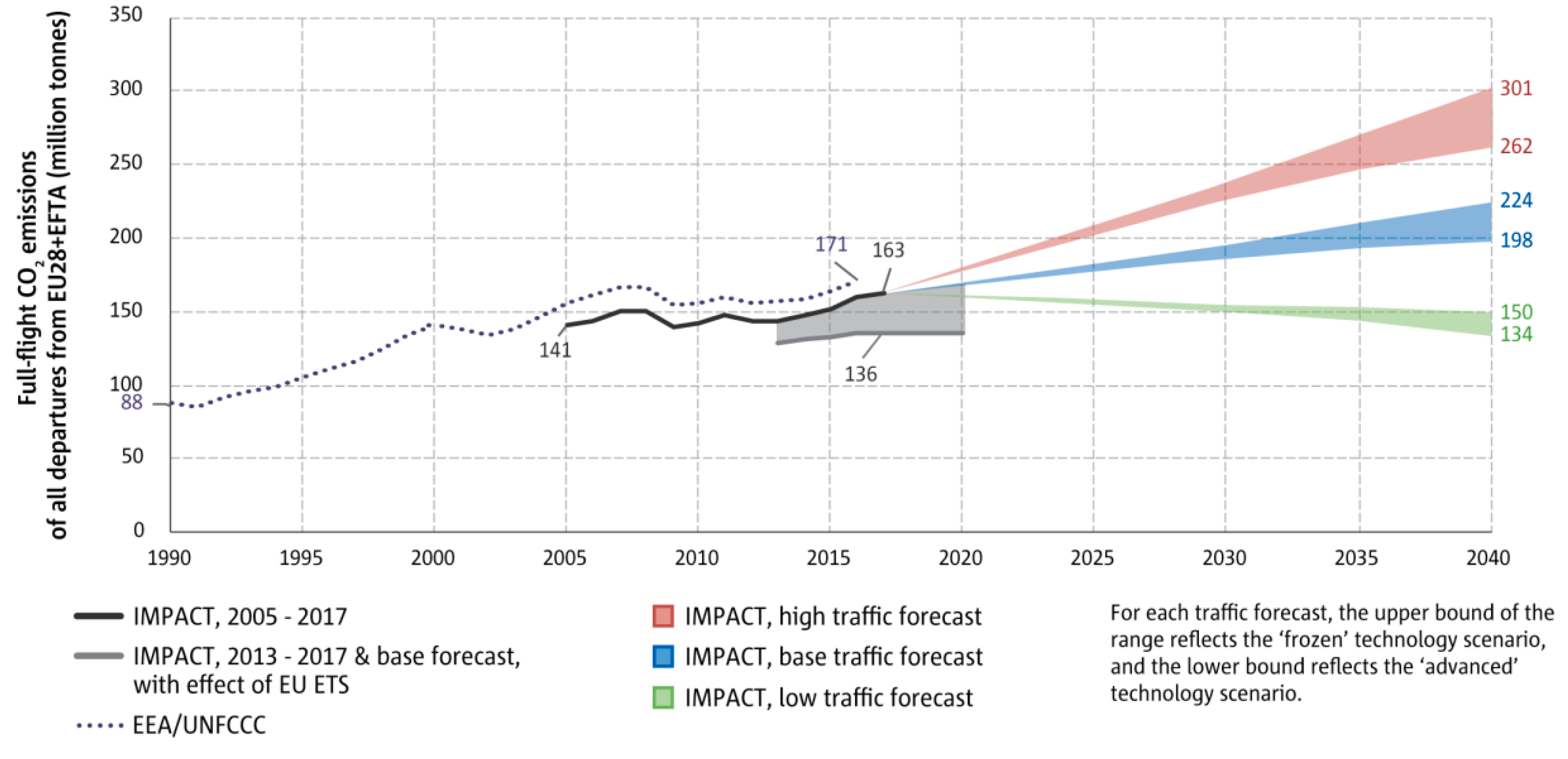
According to the data reported by members states to the United Nations Framework Convention on Climate Change (UNFCCC) and European Environment Agency (EEA), the CO₂ emissions of all flights departing from airports in the European Union (EU28) and European Free Trade Association (EFTA) increased from 88 to 171 million tonnes (+95%) between 1990 and 2016 (Figure 3). In comparison, CO₂ emissions estimated with the IMPACT model reached 163 million tonnes (Mt) in 2017, which is 16% more than 2005 and 10% more than 2014. Future CO₂ emissions under the base traffic forecast and advanced technology scenario are expected to increase by a further 21% to reach 198 Mt in 2040. The annual purchase of allowances by aircraft operators under the EU Emissions Trading System (ETS) since 2013 resulted in a reduction of 27 Mt of net CO₂ emissions in 2017, which should rise to about 32 Mt by 2020 [37].

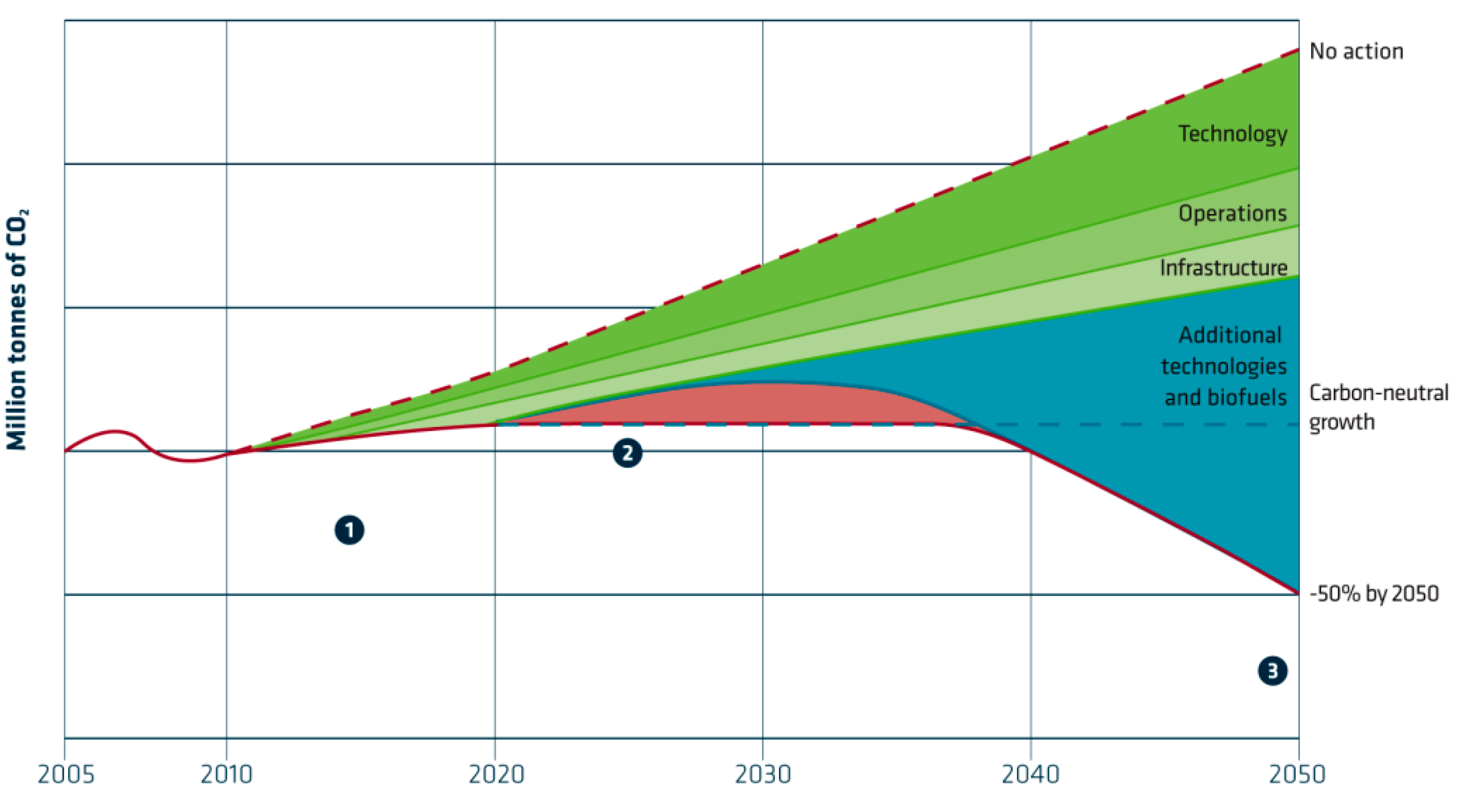
The aviation industry with its growing potential is faced with carbon-neutral growth. It is based on a signed declaration from 2008 that is known as the four-pillar strategy for reducing emissions. Those four pillars are: technology [38]; improved operational practices (including auxiliary power unit (APU) usage, weight reduction measures and more efficient flight procedures)) [39,40]; infrastructure improvements; and positive economic measures [9]. Figure 4 shows a schematic, indicative diagram dedicated to the emissions reduction roadmap [41].

CO₂ emissions are directly related to fuel burn and fuel efficiency. Therefore, world-aknown manufacturers, Airbus and Boeing, are constantly working on the development of new models based on improved aircraft efficiency. For example, a recent version, the 737–800, can carry 48% more passengers, 119% further with a 67% increase in payload, while burning 23% less fuel—or 48% less fuel on a per-seat basis. Another example shows that the latest generation Airbus A320 is around 40% less expensive—and more fuel-efficient—to operate than the aircraft it replaced. Statistics show that, Airbus spends $265 million per annum on research and development in further improving the efficiency of the A320 family of aircraft [41].

One of the biggest challenges in the aviation sector is how to perform more safely and efficiently in airspace which is shared by different users (not all aircraft operators are airlines). According to Single European Sky ATM Research Joint Undertaking (SESAR) innovative researches, new ‘flexible use of airspace’ concepts would bring savings in fuel and CO₂. For example, it is estimated that there will be 3.9 Mt fuel savings per year in 2020 and 5.6 Mt in 2030. On the other hand, it estimated 12.2 Mt CO₂ savings per year in 2020 and 17.7 Mt in 2030. It would benefit in net cost savings, for example, for jet fuel $85/b of $7.6 billions in 2020, and $10.3 billions in 2030.

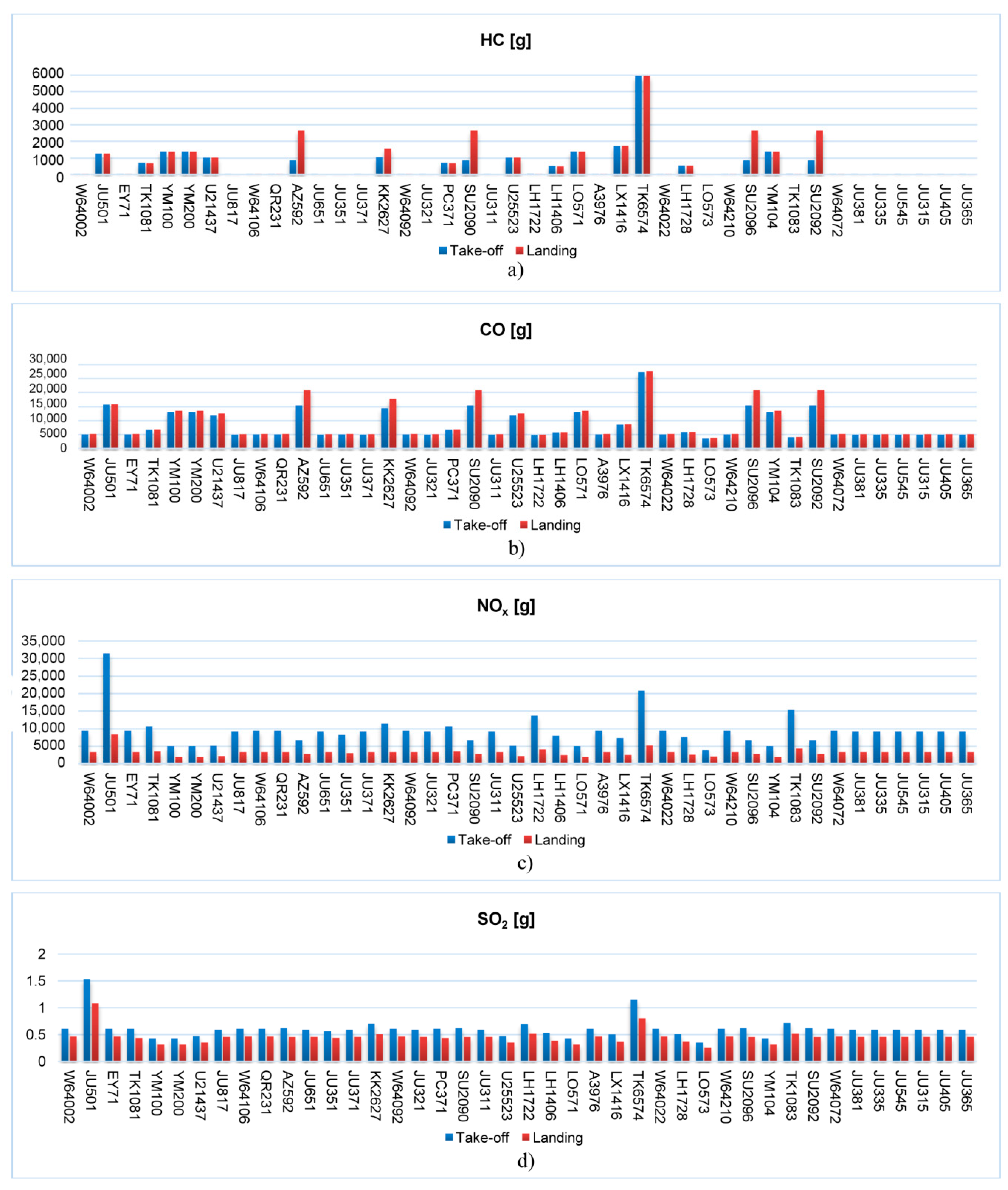
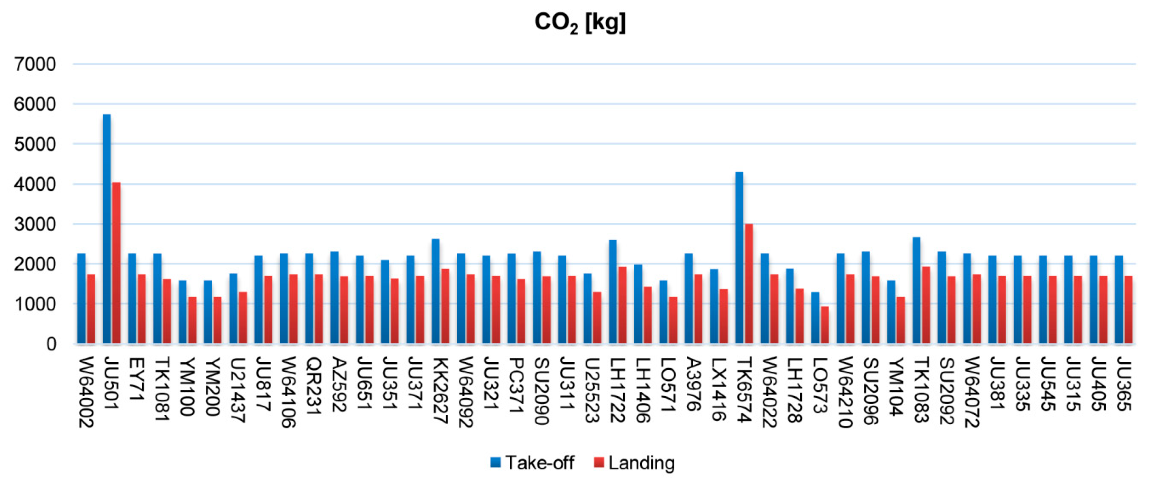
The main pollutants emitted by aircraft engines in operations are CO₂, NO_x, SO_x, HC, CO, PM and soot. This paper provides calculations in full-flight emissions of 42 flights operating from Belgrade Airport Nikola Tesla recorded on 25 January 2017 scheduled flights (

Table 3. Emissions recorded on 25 January 2017; flight No. W64072, A320-232 (engine type V2527-A5).

Flight Phase	HC	CO	NOx	CO2	SO2
Take-off	55.084	5154.963	9401.706	2267.695	0.604
Landing	51.273	5337.658	3239.76	1739.759	0.464
Total	106.357	10,492.620	12,641.466	4007.455	1.069

). Serbian flag carrier recorded the highest number of flights per day, whilst the most exploited aircraft type was A320-232, with a V2527-A5 engine.

Calculation is based on International Civil Aviation Organization (ICAO) simple approach method and ICAO Aircraft Engine Emissions Databank [42], based on aircraft type, engine and number of landing/take-off (LTO) cycles (

Table 4. Flight phase duration based on International Civil Aviation Organization (ICAO) Aircraft Engine Emissions Databank; Source: [42].

Operation		Take-Off		Landing
Flight phase	Idle	Take-off	Climb	Approach	Idle
Min	26	0.7	2.2	4	26

).

The year 2017 is used as a basis (Scenario 0—S0) with a total number of recorded aircraft operations of 58,633 (or 29,316.5 LTO cycles). For adequate comparison with the results provided in the road transport sector, the estimation was done for the two future development scenarios in the year 2032. Scenario 1 assumes the normal increasing rate on aircraft operations (1% annual rate or 68,333 aircraft operations) and Scenario 2 assumes an optimistic traffic increase rate (2.5% annual rate or 85,245 aircraft operations).

5. Results and Discussion

5.1. Road Transportation

Table 5. Traffic volumes of specific vehicle categories per different scenarios (×1000 veh-kms).

	Scenario S0 (2017)	Scenario S1 (2032)	Scenario S2 (2032)
Cars-Gasoline	2,762,439	7,516,227	8,863,494
Cars-Diesel	3,899,914	10,611,143	12,513,168
Cars-LPG	1,462,468	3,979,179	4,692,438
Buses	319,855	321,638	214,205
Trucks-Light	138,546	204,529	197,021
Trucks-Medium	386,521	570,605	549,658
Trucks-Heavy	609,288	899,468	866,448
Articulated trucks	819,745	1,210,156	1,165,732
Total all vehicles	10,398,775	25,312,945	29,062,165

shows the realised traffic volumes for all vehicle categories per different scenarios.

In Scenario S0 (2017) the total traffic volume of over 10 billion vehicle-kilometres (veh-kms) was achieved. Passenger vehicles (passenger cars and buses) have a dominant share in the total traffic volume of about 80%. Over 73% of freight traffic volume refer to articulated and heavy trucks.

In Scenario S1 (2032), it is noticeable that the total traffic volume is 2.5 times higher than Scenario S0 (2017). By category of vehicles, the biggest change is characteristic for passenger cars (growth of 172%), while the smallest change is characteristic for buses (growth by 0.56%). The freight traffic volume was increased by an average of 48%.

In Scenario S2 (2032), there was an additional generation of total traffic volume due to the implementation of development projects on the road network. Compared to Scenario S1 (2032), the volume of traffic is higher by almost 5 billion veh-kms. The increased traffic volume is only characteristic for passenger vehicles (around 18% growth compared to scenario S1 (2032)). Improving the level of service on the rail network has redistributed freight traffic flows from the road network to the rail network, and then road freight vehicles have a lower traffic volume than in Scenario S1 (2032). On average, the decreasing rate is around 3.7%. For buses, this effect is even more pronounced—the decrease in bus traffic volume is lower by as much as 33%.

Table 6. Exhaust emission costs—Scenario S0 (2017) (€/year).

Scenario S0 (2017)	CO	NOx	NMVOC	CH4	PM	CO2	SOx	Total
Cars-Gasoline	1,742,797	20,417,331	1,226,757	158,347	124,303	18,645,838	15,247	42,330,620
Cars-Diesel	105,390	26,483,584	114,947	26,180	7,370,034	23,930,544	11,703	58,042,382
Cars-LPG	627,368	12,173,843	566,359	23,455	-	8,153,279	-	21,544,303
Buses	61,850	17,516,016	95,378	19,383	1,918,138	7,383,680	3617	26,998,062
Trucks-Light	14,847	2,306,449	14,708	1691	842,400	1,732,352	848	4,913,295
Trucks-Medium	44,790	15,547,244	63,022	10,573	1,446,235	6,409,323	3140	23,524,326
Trucks-Heavy	115,128	43,797,908	166,293	31,708	3,625,619	15,828,085	7757	63,572,498
Trucks-Articulated	210,126	79,525,253	320,972	59,083	6,806,008	26,379,050	12,915	113,313,407
Total all vehicles	2,922,294	217,767,627	2,568,437	330,419	22,132,737	108,462,152	55,228	354,238,894

,

Table 7. Exhaust emission costs—Scenario S1 (2032) (€/year).

Scenario S1 (2032)	CO	NOx	NMVOC	CH4	PM	CO2	SOx	Total
Cars-Gasoline	2,742,238	16,286,416	2,721,032	452,190	217,021	105,407,202	13,283	127,839,381
Cars-Diesel	165,186	22,291,190	62,142	18,138	4,341,423	134,922,674	8474	161,809,227
Cars-LPG	948,672	9,764,658	1,137,303	60,472	-	43,911,296	-	55,822,400
Buses	89,433	3,052,375	24,199	7180	651,978	16,008,739	1007	19,834,911
Trucks-Light	16,716	889,657	6118	928	219,842	4,742,587	298	5,876,147
Trucks-Medium	59,801	4,207,598	26,476	6108	721,289	19,724,897	1241	24,747,410
Trucks-Heavy	250,726	10,479,647	65,825	16,176	1,818,529	48,765,516	3069	61,399,490
Trucks-Articulated	476,868	17,582,344	122,714	29,476	3,525,749	81,286,635	5111	103,028,896
Total all vehicles	4,749,641	84,553,885	4,165,807	590,668	11,495,831	454,769,545	32,484	560,357,862

and

Table 8. Exhaust emission costs—Scenario S2 (2032) (€/year).

Scenario S2 (2032)	CO	NOx	NMVOC	CH4	PM	CO2	SOx	Total
Cars-Gasoline	2,846,034	17,442,992	2,676,760	444,832	222,923	109,204,778	13,762	132,852,081
Cars-Diesel	173,607	25,217,141	62,726	18,309	4,306,707	142,260,675	8935	172,048,100
Cars-LPG	1,011,157	10,739,497	1,145,169	60,890	-	46,709,059	-	59,665,772
Buses	49,888	1,356,880	12,828	3806	331,651	8,949,034	563	10,704,650
Trucks-Light	13,993	779,495	5079	771	156,596	3,977,809	250	4,933,994
Trucks-Medium	44,130	2,600,112	18,684	4311	480,583	14,597,980	918	17,746,717
Trucks-Heavy	185,055	6,480,873	46,245	11,364	1,207,963	36,112,298	2273	44,046,071
Trucks-Articulated	351,128	11,054,637	87,049	20,909	2,369,736	60,020,321	3774	73,907,554
Total all vehicles	4,674,992	75,671,626	4,054,541	565,192	9,076,159	421,831,954	30,475	515,904,939

show exhaust emission costs for different vehicle categories according to different scenarios.

In Scenario S0 (2017), the total exhaust emission costs are around 354 million €. The largest share (over 60%) belongs to the costs of nitrogen oxide emissions. The main reason for this is the current age of the road vehicles in Serbia (about 16 years) (i.e., the higher emission factors of this pollutant, especially for buses and all sub-categories of freight vehicles) (Table 7). The costs of carbon dioxide emissions are about 30% of the total costs and depend directly on fuel consumption. Although PM unit costs are very high, due to relatively small emission factors, these costs have a share of 6.25% in total costs. The costs of other pollutants (CO, NMVOC, CH₄, SO_x) are below 1%, in total of about 6 million €.

Scenarios S1 (2032) include the “modernization” of the road vehicle fleet, with emission factors significantly lower than in the case of Scenario S0 (2017). However, due to increased total traffic volume, exhaust emission costs are 58% higher than Scenario S0 (2017) and amounts to 560 million €. Observing all vehicle categories, the average exhaust emission costs per 100 km are about 2.2€ (in Scenario S0 (2017) this value is about 3.4€). Drastic reduction of emission factors of nitrogen oxides results that in the total costs, the largest share has carbon dioxide emission costs, over 80%. The relatively high unit cost of nitrogen oxides and a larger quantity of emissions compared to other pollutants causes a share of nitrogen oxides emission costs in the total value of about 15%.

In Scenario S2 (2032), 13 development projects were implemented on the road network. Improvements in road conditions led to an increase in the level of service, that is, to the reduction of congestions on the road network. Due to the increase in the capacity on some road sections, the flow/capacity ratio is lower and operational speeds are increased compared to the conditions in Scenario S1 (2032). The consequence of improvement of road and traffic conditions is that with the increased traffic volume of 15% compared to Scenario S1 (2032), lower total exhaust emission costs are realized. The total amount is 515 million €. The exhaust emission costs per 100 km are significantly lower than the previous two scenarios and are around 1.8€. The share of the exhaust emission costs of individual pollutant in total costs is very similar to Scenario S1 (2032) (i.e., CO₂ emissions costs are the main generators of total emissions costs). Average CO₂ emissions costs per 100 km are lower by 0.35 euro cents in comparison to the same costs in Scenario S1 (2032), which indicates that the average fuel consumption at the level of whole network is lower than in Scenario S1 (2032).

5.2. Air Transportation

Based on the provided methodology, total emissions per flight phase on 25 January 2017 are presented in Figure 5, Figure 6, Figure 7 and Figure 8.

The provided analysis shows that the largest quantity of harmful substances (i.e., sulfur oxide, nitrogen oxide, carbon dioxide, etc.) emits from aircraft A310-308F with engine type CF6-80C2A8 and A330-243 with engine type TRENT 772C-60.

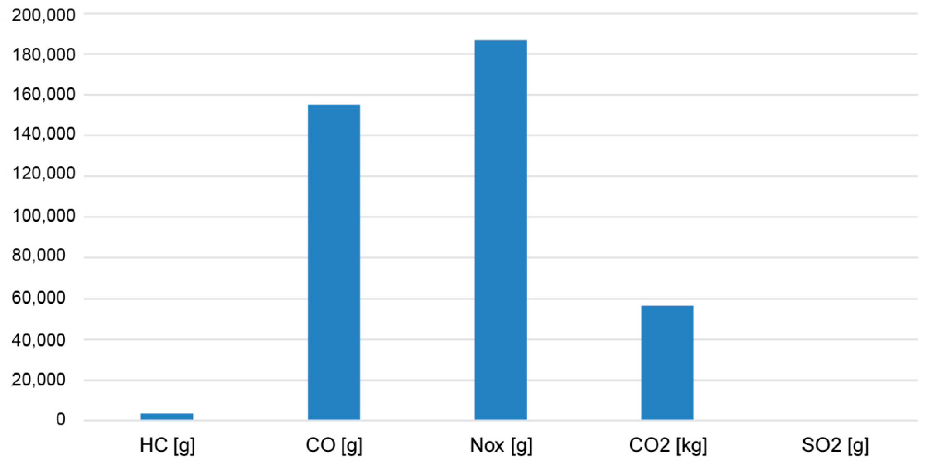
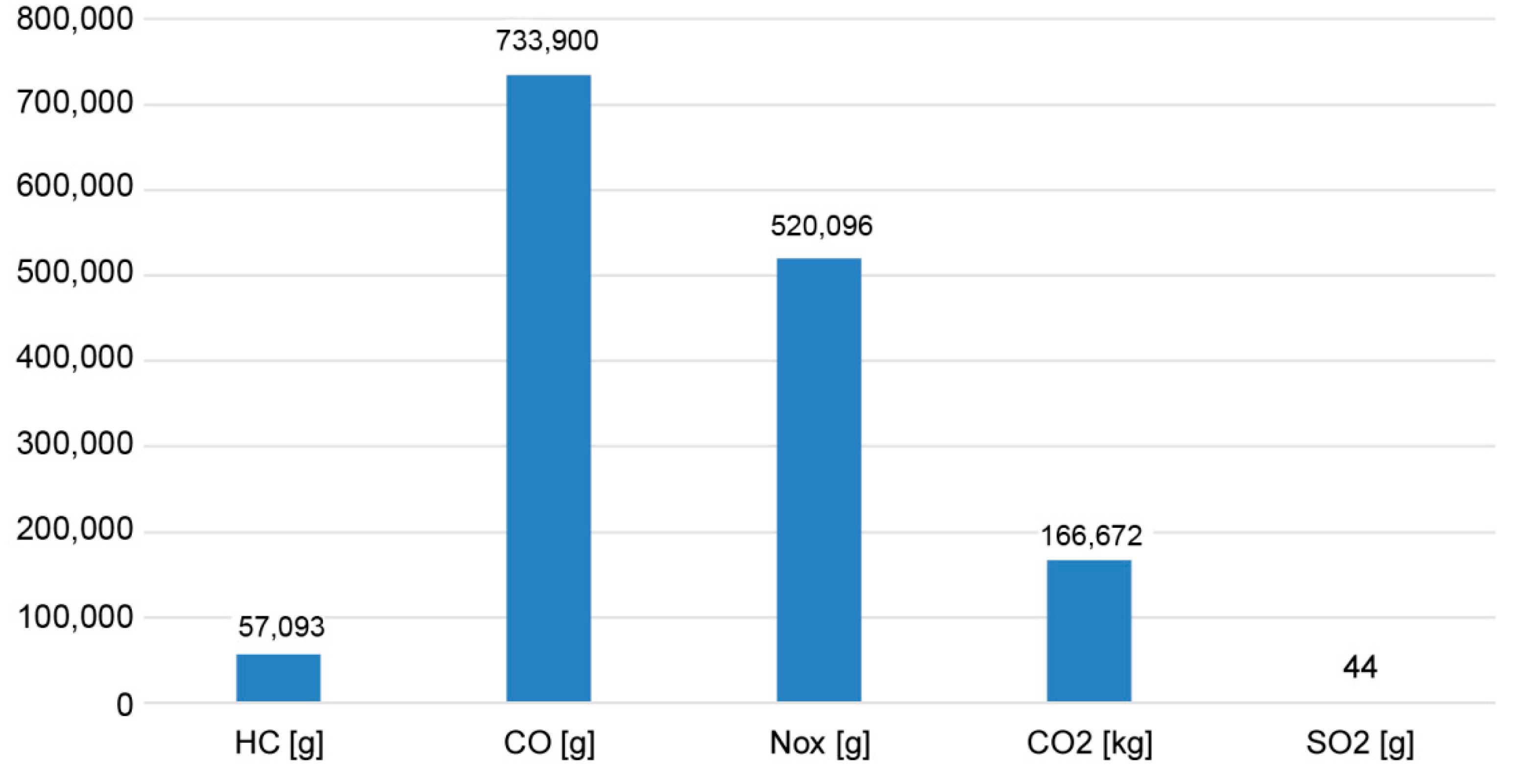
Moreover, emissions from the national airline fleet and the share in total emissions is calculated as follows:

• 6.5% of the total HC emissions;
• 21% of the total CO emissions;
• 36% of the total NO_x emissions;
• 34% of the total CO₂ emissions;
• 34% of the total SO₂ emissions.

Since the most present aircraft type in airport operations is A320, the following calculation is based on its engine type and exhausted emissions. Considering data collection and obtained results, estimation of the cost of CO₂ and other aircraft emissions released by the combustion of aviation fuel could be done in accordance with [43]. This document is based on recommended sources and defined values from the European Energy Exchange AG (EEX), Germany’s energy exchange, which is the leading energy exchange in Central Europe and from the update of the Handbook on External Costs of Transport [44].

The presented analysis shows that Scenario 1 increases total emission costs by 68.85% whilst Scenario 2 increases total emission costs by 110.65% (

Table 9. Total emissions costs recorded in 2017, 2032 (Scenario 1) and 2032 (Scenario 2) (€/year).

Representative Engine (CFM56-5B4/2)	HC	CO	NOx	CO2	SO2	Total Annual Costs (€)	Total Annual Costs (€) [43]
per landing/take-off (LTO) (g)	2700	22,468	7566	2,825,040	1540
Total annual emissions (tonne)-2017	79.45965	661.222	222.6636	83,139.51468	45.32143
Emissions costs (Unit costs) 2017 (€/tonne)	563.09	106.5	10,052.22	35.5	9199.13
Total emissions costs-2017 (€)	44.742.93	70,420.14	2,238,263	2,951,452.771	416,917.7	5,721,797.038	4,767,579
Total annual emissions (tonne)-2032-Scenario 1	92.24955	767.6529	258.5037	96,521.72916	52.61641
Total annual emissions (tonne)-2032-Scenario 2	115.0808	957.6423	322.4818	120,410.2674	65.63865
Emissions costs (unit costs) 2032 (€/tonne)	700.53	174	12,594.45	58	11,581.08
Total emissions costs-2032-Scenario 1 (€)	64,623.58	133,571.6	3,255,712	5,598,260.291	609,354.9	9,661,522.746	9,908,285
Total emissions costs-2032-Scenario 2 (€)	80,617.52	166,629.8	4,061,481	6,983,795.509	760,166.5	12,052,690.6	12,360,525

).

EUROCONTROL [43], provides the EU average for marginal air pollution costs for passenger aviation regarding distance group and aircraft type.

Table 10. Average aviation emission costs [43].

Distance Group	Type of Aircraft	Range	Typical Number of Seats	Average Capacity Utilization	Air Pollution Costs
					€/LTO	€ cent/km
Short-haul	Fokker 100	<1000 km	85	65%	81	0.29
Medium-haul	Airbus A320	<3700 km	150	70%	145	0.05
Long-haul	Boeing 747-400	>3700 km	416	80%	702	0.03

presents those emission costs. According to Table 9 and recorded and forecasted number of operations, it is possible to make a comparison regarding those two approaches.

With regards to the NO_x charges, an LTO NO_x charge is currently made at several European airports and primarily targets local air quality. The level of the charge per kg of NO_x is set at the local air quality (LAQ) damage costs of NO_x locally, at or around airports. The charge is levied today in several countries: Sweden, England, Germany, Demark and Switzerland. For example [37]: at London Heathrow, the emissions charge per kg of NO_x for fixed wing aircraft over 8618 kg was £8.82 (approx. €12) on 1 July 2014. Another example is recorded in Sweden in May 2016, where the emissions charge for aircraft exceeding 5700 kg is set at SEK 50 (approx. €5.33) per kg of NO_x (for the sum of all 4 LTO modes: approach, taxi, take-off and climb).

6. Conclusions

The calculation of the exhaust emission costs for the road transport shown in this paper takes into account a large number of influential factors: changing of traffic volumes, changing of design and operating speeds, the mutual interaction of vehicles in the traffic flow, the quality of the pavement structure, the type of terrain of a road section, the category of road sections and the dependence of the exhaust emission from changes in vehicle speed. On the basis of the above, the following conclusions can be drawn.

Current exhaust emission costs in the road transport sector are mostly based on the emissions costs of nitrogen oxides. The primary reason is the high emission factors of NO_x for all vehicle categories due to the obsolescence of the road vehicle fleet in Serbia. The secondary reason is the relatively high unit cost of nitrogen oxides. In 2017, freight vehicles generate 57% of the total exhaust emissions costs.

In 2032, the increase in the traffic volume and non-investing in the road transport infrastructure will result in an increase in the total exhaust emission costs compared to 2017. A reduction in emission factors, especially for freight road vehicles, is expected, and this will result in lower average emissions costs per 100 km than in 2017 by 35%. The share of passenger car exhaust emission costs in the total emission costs is dominant and amounts to 65%.

With the implementation of development projects in 2032, the total exhaust emission costs in the road transport sector and therefore the average exhaust emission costs per 100 km are reduced. Due to the use of other modes of transport, the freight traffic volume realized on the road network is decreasing. Consequently, the emission costs of passenger cars are even more pronounced in the total emission cost with a value of 72%.

The general conclusion is that the future use of various exhaust gas treatment devices (three-way catalysts, oxidation catalysts, diesel particulate (DP) filters) will lead to a significant reduction in emissions and emission costs of nitrogen oxides, particulate matters and carbon monoxide. This will affect the fact that the dominant pollutant, in terms of generating of exhaust emission costs in the next years in the road transport sector, will be carbon dioxide. In the forecasted time period, the share of carbon dioxide emissions in total exhaust emission costs will exceed 80% and will mainly be generated by passenger cars.

The calculation of the exhaust emission costs for air transport shown in this paper considers a large number of influential factors: airport capacity, number of operations, aircraft type, relevant engine and range. On the basis of the above, the following conclusions can be drawn.

The dominant pollutant in the air transport sector is carbon dioxide since the general approximation shows that one kilogram burned aircraft fuel generates 3.16 kg of CO₂. Another higher pollutant is nitrogen oxide with a total share of 39% of the total exhausted costs. Nowadays, only several countries within Europe provide market measures for NO_x and most efforts are focused on CO₂ carbon neutral growth and −50% reductions by 2050.

Those goals require a variety of measures based on: known technology, operations and infrastructure measures, bio-fuels and additional new generation technologies and economic measures. The provided research is a good platform for economic measures and therefore, it provides a forecast of the number of aircraft operations, emission costs and pollutants based on two independent sources. Comparing the provided results, it could be found that the average exhaust emission costs per one aircraft operation will range from 141 to 145€ in 2032.

The provided research could be used as a roadmap to calculate exhaust emission costs for other European airports based on the set future development scenario.