Abstract
Error propagation properties of integration algorithms are crucial in conducting pseudodynamic tests. The motivation of this study is to investigate the error propagation properties of a new family of model-based integration algorithm for pseudodynamic tests. To develop the new algorithms, two additional coefficients are introduced in the Chen-Ricles (CR) algorithm. In addition, a parameter—i.e., degree of nonlinearity—is applied to describe the change of stiffness for nonlinear structures. The error propagation equation for the new algorithms implemented in a pseudodynamic test is derived and two error amplification factors are deduced correspondingly. The error amplification factors for three structures with different degrees of nonlinearity are calculated to illustrate the error propagation effect. The numerical simulation of a pseudodynamic test for a two-story shear-type building structure is conducted to further demonstrate the error propagation characteristics of the new algorithms. It can be concluded from the theoretical analysis and numerical study that both nonlinearity and the two additional coefficients of the new algorithms have great influence on its error propagation properties.
1. Introduction
In the field of civil engineering, experimental studies are crucial to investigate and enhance the sustainability and resilience of civil infrastructures in the event of extreme loads, such as earthquakes. The experimental approaches of studying the seismic performance of building structures include the quasi-static tests, shake table tests, pseudodynamic tests, and real-time hybrid simulations. Among them, the pseudodynamic tests, also known as on-line tests or hybrid simulations, have been paid great attention for decades [1,2].
In conducting a pseudodynamic test, two types of errors—i.e., displacement control error and restoring force measurement error—introduced in each time step will be propagated and accumulated owing to a feedback procedure [1,2]. This feedback procedure roots from the use of an integration algorithm to conduct the step-by-step integration during the pseudodynamic test. Therefore, it is crucial to investigate the error propagation of an integration algorithm because the errors from the pseudodynamic test must be controlled within certain limits to obtain reliable test results.
An integration algorithm can be labeled as explicit or implicit depending on its formulation of displacement. Traditional explicit algorithms, such as the Newmark explicit algorithm, are always conditionally stable, which requires a very severe limitation on the integration time step if the tested structure system has high frequency modes [3]. For the past decade, researchers developed several innovative integration algorithms which are both explicit and unconditionally stable. The representative algorithms include the Chang algorithm [4], the Chen-Ricles (CR) algorithm [5], and the Kolay-Ricles-𝛼 (KR-α) algorithm [6]. These algorithms are nominated as model-based integration algorithms [7]. When using these algorithms, the algorithmic parameters, which are functions of the complete model of the system, have to be calculated. The model-based algorithms can achieve unconditional stability within the framework of an explicit formulation. On the contrary, there is no need to calculate the model-based parameters for the conventional integration algorithms such as the well-known Newmark algorithms, so they are called model-independent algorithms. Although a number of studies [8,9,10,11,12,13,14,15] have been conducted for the error propagation of the model-independent integration algorithms, there is very limited research with regard to the error propagation of the model-based integration algorithms.
In addition, most of the previous work [8,9,10,11,12] on the error propagation of the integration algorithms were conducted for linear elastic systems. Only a few research [13,14,15] were aimed at nonlinear structures. It should be noted that most of the pseudodynamic tests were carried out in nonlinear range of behavior as pseudodynamic tests are mainly used to investigate the nonlinear behavior of the structures subjected to seismic excitations [2,16]. Therefore, it is much more meaningful to perform the nonlinear error propagation analysis. To take the nonlinearity into consideration, the degree of nonlinearity, which was adopted in [13,14,15], is introduced in this study. Furthermore, the influence of viscous damping, which is a critical structural parameter, on the error propagation characteristics have not been considered in the previous studies [13,14,15].
The motivation of this study is to investigate the error propagation properties of a new family of model-based integration algorithm for pseudodynamic tests of nonlinear systems by considering the influence of viscous damping. The new family of model-based integration algorithms is firstly introduced in Section 2. The procedure of using the new algorithms in pseudodynamic tests is then presented in Section 3. The error propagation equation and two error amplification factors for the new algorithms are derived in Section 4 (Appendix Figure A1 shows flowchart of calculating the error amplification factors). To further illustrate the influences of the degree of nonlinearity, viscous damping, and two additional coefficients of the new algorithms, the error amplification factors derived from Section 4 for three structures with different degrees of nonlinearity are obtained to demonstrate the error propagation effect in Section 5. Finally, the numerical simulations of pseudodymamic tests for a two-story shear-type building are also conducted to further illustrate the error propagation properties of the new algorithms in Section 6.
2. A New Family of Model-Based Integration Algorithm
In implementing a pseudodynamic test, the structure must be idealized as a discrete model, whose equation of motion can be written as
where M, C, and K are mass, damping and stiffness matrices, respectively; , , and are displacement, velocity, and acceleration vectors at the (i + 1)th time step, respectively; and is the external force vector at the (i + 1)th time step.
The integration algorithms can be used to solve the equation of motion (Equation (1)) in conducting a pseudodynamic test. Recently, the authors [17] proposed a new family of explicit integration algorithm, which was a generalized version of the CR algorithm [5], which was proposed by Chen and Ricles and has been successfully implemented in a series of real-time hybrid simulation tests. The new family of algorithms is named ‘generalized CR algorithm’ and is abbreviated as ‘GCR algorithm’ in this paper. The formulation of the GCR algorithm is inherited from the CR algorithm and expressed as
where is the time step; and are the integration parameter matrices
where and are two additional coefficients controlling the numerical characteristics of the GCR algorithm. The CR algorithm is the special case of the GCR algorithm with .
It can be concluded from the preliminary study [17] that the subfamily of the GCR algorithm with has no numerical damping, while the subfamily of the GCR algorithm with has numerical damping. The GCR algorithm is superior to commonly used integration algorithms due to its explicit expressions and unconditionally stability. In addition, the numerical characteristics of the GCR algorithm are identical with the well-known Newmark algorithm. Therefore, the GCR algorithm can be easily adopted in solving the equation of motion in the pseudodynamic tests and other structural dynamic problems.
For the brevity of mathematics, the following derivations are only considered for a single-degree-of-freedom (SDOF) system. As for the SDOF system, all the matrices and vectors in Equations (1)–(3) become scalars.
The degree of nonlinearity used in [13,14,15] is introduced to evaluate the change of stiffness for the nonlinear system and defined as
It should be noted that means the stiffness remains unchanged during the (i + 1)th time step, while and can be used to represent the nonlinear system with stiffness hardening and the stiffness softening during the (i + 1)th time step, respectively.
3. Pseudodynamic Test Procedure
Because there are possible variations in the changes of stiffness and the resulting complicated eigendecomposition, it is almost impossible to conduct the error propagation analysis for the whole step-by-step integration procedure. Therefore, only a specific time step is analyzed for the error propagation analysis of a nonlinear system [13].
It should be noted that the GCR algorithm is a dual-explicit algorithm, which means it is explicit for both displacement and velocity, so the pseudodynamic test procedure is much easier and more direct compared to the pseudodynamic test using the Newmark explicit algorithm [13], the subfamily of Hilber-Hughes-Taylor-𝛼 (HHT-𝛼) algorithm [14] or the constant average acceleration method [15].
The step-by-step integration procedure for the GCR algorithm can be written in a recursive matrix form. It is
where . The amplification matrix and the load vector for the (i + 1)th time step are
where and is the natural frequency of the system at the end of the (i + 1)th time step. is the equivalent viscous damping ratio, where is the initial natural frequency of the system. Differing from the work conducted by other researchers [13,14,15], the influence of viscous damping is also taken into consideration in this study.
After the eigendecomposition of the matrix , its characteristic equation can be obtained by the equation of and expanded as
where I is the identity matrix of dimension 3 × 3; λ is the eigenvalue of the matrix ; ; . It is apparent that there are three eigenvalues and one of them is zero, so the above equation can be further simplified as
There are two eigenvalues . According to [17], the condition of the unconditionally stable GCR algorithm can be derived
Therefore, the error propagation characteristics of the subfamily of the unconditionally stable GCR algorithm is investigated in the following content.
4. Derivation of Error Propagation Equation
In conducting a pseudodynamic test, control and measurement errors are unavoidable and are introduced at each time step. Firstly, it is very difficult to exactly impose the computed displacement on the specimen because of the displacement control error. Secondly, the restoring force actually developed in the specimen may not be correctly measured. These errors are carried over to the subsequent time steps and exhibit a cumulative effect from the beginning to the end of the test.
The equation of motion of a nonlinear SDOF system is
where is the restoring force at the (i + 1)th time step. The displacement and velocity calculated from the SDOF formulation of Equation (2) are accurate values, and the corresponding restoring force obtained by state determination is also accurate and without error.
The below two equations define the actual displacement and restoring force during a pseudodynamic test [13]:
where and are the actual displacement and restoring force at the (i + 1)th time step, respectively, including the effects of errors at previous steps and the current step; and are the exact displacement and restoring force at the (i + 1)th time step, respectively, including the effects of errors at previous steps; and are the displacement error and the restoring force error at the (i + 1)th time step, respectively.
The restoring force error at the (i + 1)th time step can be further expressed as [13]
where is the displacement error corresponding to the restoring force error . According to the above definition and the formulations of the GCR algorithm, the following relationships can be obtained
It should be noted that , so the aforementioned equations can be reformulated in a recursive matrix form [13]
where ; ; .
Subtracting Equation (5) from Equation (16), the following error propagation equation can be obtained
Define , then the error propagation equation can be rewritten as
The error cumulative vector can be explicitly expressed as
It is obvious that is the cumulative displacement error for the (i + 1)th time step. When the specimen enters into a nonlinear range, the amplification matrix and vectors and are varied for each time step, so it is almost impossible to calculate the cumulative displacement error for a complete pseudodynamic test such as that developed by Shing and Mahin [11] for a linear elastic system. Even so, if the error propagation for a specific time step is thoroughly studied, some useful information can still be acquired. Therefore, the error propagation from the previous one and two time steps to the current time step is derived as follows.
After the repeated substitutions of and into using Equation (20), the following cumulative equation can be acquired
It is assumed that is mainly affected by and , while less affected by , then the item of can be omitted and the cumulative equation can be further simplified as
where and are the cumulative error vector caused from the displacement feedback errors and restoring force feedback errors.
Substituting the amplification matrix into Equation (22), the cumulative displacement error for the (i + 1)th time step can be expressed as
As the coefficients , , , , and , of Equation (23) are so complicated, they are not exhibited in the paper. However, it is very convenient to numerically calculate them by using MATLAB [18]. Equation (23) can be further expressed as
where and are the phase angles, and are the displacement and restoring force error amplification factors arising from the previous one and two steps to the cumulative displacement error, respectively. These two amplification factors are all dimensionless and widely used to evaluate the error propagation properties of the integration algorithms in pseudodynamic tests [10,11,12,13,14,15]. The expressions of the two factors for the GCR algorithm are
5. Examples for Error Propagation Effect
The aforementioned two error amplification factors, i.e., the displacement error amplification factor (Equation (25)) and the restoring force error amplification factor (Equation (26)), are used to illustrate the error propagation effect of the GCR algorithm. The degree of nonlinearity is used to define three cases as:
(1) Case 1: nonlinear structure with stiffness softening,
(2) Case 2: linear elastic structure,
(3) Case 3: nonlinear structure with stiffness hardening,
Figure 1 and Figure 2 show the two error amplification factors, i.e, and , with respect to the initial , respectively.
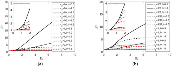
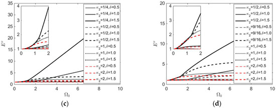
Figure 1.
Variations of displacement error amplification factor with respect to : (a) ; (b) ; (c) ; (d) .
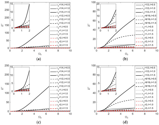
Figure 2.
Variations of restoring force error amplification factor with respect to : (a) ; (b) ; (c) ; (d) .
It can be seen from Figure 1 and Figure 2 that both amplification factors and increase with . This result is in consistent for those of other integration algorithms [10,11,12,13,14,15]. Besides, both amplification factors increase with the degree of nonlinearity δ, which is in line with the observations from [13,14,15]. It indicates that the degree of nonlinearity has a significance influence on the error propagation properties of the GCR algorithms. More specifically, the nonlinear structures with stiffness hardening possess the most errors, while the nonlinear structures with stiffness softening have the lowest errors. As for the viscous damping, it has a positive effect on reducing the errors. Therefore, it is conservative to ignore the influence of viscous damping. Both the two additional coefficients—i.e., and —of the GCR algorithms have great impact on the error propagation property. With the increasing of , the errors increase, while both amplification factors and increase with the decrease of . In terms of error propagation, it is recommended to select the GCR algorithms with a small value of and a large value of . For instance, it is superior to use the GCR algorithm with than the original CR algorithm with in a pseudodynamic test, especially for the nonlinear structures with stiffness hardening. Taking the structure of Case 3 without viscous damping () as an example, the displacement amplification factors of the GCR algorithm with and the original CR algorithm with are 2.43 and 4.33 (=1.78 × 2.43), respectively, for , and are 3.56 and 32.91 (=9.24 × 3.56), respectively, for (Figure 1a). The restoring force amplification factors of the GCR algorithm with and the original CR algorithm with are 4.69 and 14.76 (= 3.15 × 4.69), respectively, for ; are 11.55 and 251.80 ( = 21.80 × 11.55), respectively, for (Figure 2a). It can be clearly seen that the differences between the two specific algorithms rapidly increase with .
6. Numerical Simulation of Pseudodynamic Testing
A two-story shear-type building structure is taken as the numerical simulation example of the pseudodynamic testing. The lumped masses of the two stories are and , respectively. The initial stiffness of the two stories are and , respectively. The damping matrix for the substructure is based on using Rayleigh proportional damping [19], with a damping ratio of 0.02 in both the first and second modes. The natural initial circular frequencies for the first and second modes are found to be and , respectively. The first two order of initial frequencies are and , respectively. The structure is subjected to the 1940 El Centro NS earthquake ground motion.
In order to take the influence of error into consideration, displacement error is introduced to the displacement response at each story. Assume the displacement error is a random variable which obeys the truncated normal distribution with the probability density function as [20]
where μ and σ are the mean value and the standard deviation of the displacement error x, respectively. In conducting the pseudodynamic testing, it is assumed that μ = 0 and σ = tol/3 = 10−5 m. tol is the tolerance error and assigned as 3 × 10⁻⁵ m in this paper. It denotes that the maximum displacement error of each time step is 3 × 10⁻⁵ m. By using the MATLAB software [18], a series of random numbers conforming the aforementioned distribution can be generated and used as the displacement errors.
Numerical simulation of two situations—i.e., without displacement error and with random displacement error—using the GCR algorithm are conducted. The time step Δt is assigned as 0.01 s. As a result, and . Figure 3, Figure 4 and Figure 5 show the displacement response, displacement error at each time step, and cumulative displacement error of each story, respectively. The numerical results using the Newmark explicit algorithm with the time step of 0.001 s are used as references.
Figure 3.
Displacement response: (a) , first story; (b) , second story; (c) , first story; (d) , second story.
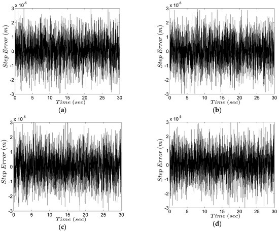
Figure 4.
Displacement error at each time step: (a) , first story; (b) , second story; (c) , first story; (d) , second story.
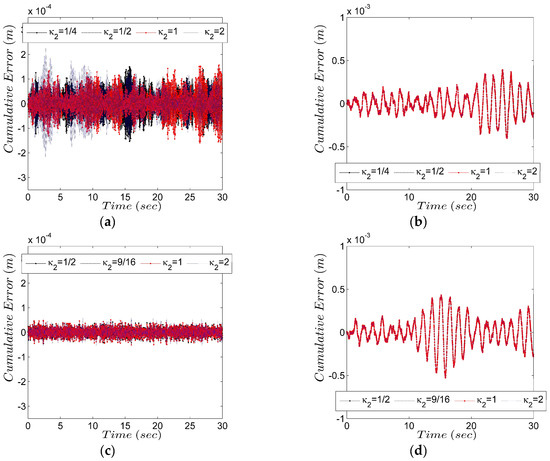
Figure 5.
Cumulative displacement error: (a) , first story; (b) , second story; (c) , first story; (d) , second story.
It can be seen from Figure 3 that the displacement response at the first story is significantly disturbed by the error. On the contrary, the influence of error on the displacement response at the second story is inconspicuous. The main reason is that the displacement at the second story is mainly contributed by the first order modal response, while the displacement at the first story is, to some extent, contributed by the second modal response, whose value of Ω is larger than that of the first modal response and therefore exhibits a higher error propagation result.
Although the cumulative displacement error can be significantly reduced with the increase of , the accurate displacement response at first story is still overlapped by the error (Figure 5a,c). As for , the displacement at the second story is in good agreement with the reference value and less affected by the displacement error (Figure 3b). As for , the displacement at the second story is also less affected by the displacement error, but the accuracy of the numerical result is impaired due to the existing of numerical damping of the integration algorithm (Figure 3d). The maximum displacement (0.094 m) at the second story calculated using the GCR algorithms with are 83% of the reference value (0.113 m).
Figure 6 shows the spectral characteristic of the displacement by conducting fast Fourier transform (FFT) of the displacement response shown in Figure 3.
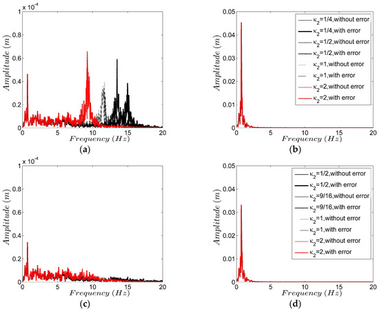
Figure 6a implies that the displacement at the first story is contributed by the first and second order of modal responses. The first order frequency obtained by several GCR algorithms are very close and approximately 0.7060 Hz, which is slightly smaller than the first order frequency of the structure, i.e., 0.7114 Hz. This is due to period elongation [19] of the integration algorithm. However, there exists obvious difference of the second order frequency between the calculated value by using several GCR algorithms and the actual frequency as period elongation increases with the increase of Ω. In Figure 6c, the first order response is obvious, while the second order response is less obvious. The reason for this is the numerical damping and the random displacement error. By comparing Figure 6b,d, the displacement at the second story is only contributed by the first order modal response, which further explains the phenomenon shown in Figure 3. In addition, due to the existing of numerical damping, the spectral amplitude of is less than that of , which is consistent with the displacement response indicated in Figure 3.
7. Conclusions
This paper presents a new family of model-based GCR integration algorithm. The error propagation equation for the GCR algorithms implemented in a pseudodynamic test is derived. The error amplification factors for three structures with different degrees of nonlinearity are calculated to illustrate the error propagation effect. The numerical simulation of a pseudodynamic test for a two-story shear-type building structure is conducted to further demonstrate the error propagation characteristics of the new algorithms. The original contributions of this study are to investigate the error propagation properties of the GCR algorithms for pseudodynamic tests of nonlinear systems by considering the influence of viscous damping. The following conclusions can be drawn from the examples and numerical simulations in Section 5 and Section 6:
- (1)
- Both amplification error factors, i.e., and , increase with .
- (2)
- Both amplification factors, i.e., and , increase with the degree of nonlinearity δ, so it is crucial to take the degree of nonlinearity δ into consideration.
- (3)
- As for the viscous damping, it has a positive effect on reducing the errors, so it is conservative to ignore the influence of viscous damping.
- (4)
- Both the two additional coefficients, i.e., and , of the GCR algorithms have great impact on the error propagation property. With the increasing of , the errors increase, while both amplification factors and increasing with the decrease of .
- (5)
- The original CR algorithm with has a relatively large error propagation property, especially for the nonlinear structures with stiffness hardening. The two amplification error factors, i.e., and , of the GCR algorithm with are only 10.8% and 4.6% of those of the original CR algorithm with when for the nonlinear structure with stiffness hardening of Case 3 without viscous damping. Therefore, the GCR algorithm with is a superior alternative of the original CR algorithm with .
- (6)
- The displacement response at the first story is significantly disturbed by the error, whereas the influence of error on the displacement response at the second story is inconspicuous. The main reason is that the displacement at the second story is mainly contributed by the first order modal response, while the displacement at the first story is, to some extent, contributed by the second modal response.
- (7)
- The maximum displacement at the second story obtained by using the GCR algorithms with are 83% of the reference value. It means that the accuracy of the numerical result is impaired by excessive numerical damping for the high frequency response, thus the numerical dissipation characteristics of the GCR algorithms should be optimized in the future.
Author Contributions
B.F. conducted the numerical simulations and wrote the paper. H.J. conceived the idea and revised the paper. T.W. provided valuable discussions and revised the paper. He took responsibility of the corresponding work.
Funding
Financial support from the National Natural Science Foundation of China (Grant No. 51578072, 51478354), Shaanxi Province Natural Science Foundation (Grant No. 2018JQ5078) and Program of Shanghai Subject Chief Scientist (18XD1403900) are gratefully acknowledged.
Conflicts of Interest
The authors declare no conflict of interest.
Appendix A: Notations
M: Mass matrix
C: Damping matrix
K: Stiffness matrix
: Displacement vector at the (i + 1)th time step
: Velocity vector at the (i + 1)th time step
: Acceleration vector at the (i + 1)th time step
: External force vector at the (i + 1)th time step
: Time step
and : Integration parameter matrices
and : Additional coefficients of the GCR algorithm
: Degree of nonlinearity
: Amplification matrix at the (i + 1)th time step
: Load vector at the (i + 1)th time step
: Natural frequency of the system at the (i + 1)th time step
: Initial natural frequency of the system
: The product of natural frequency at the (i + 1)th time step multiplies time step
: The product of initial natural frequency multiplies time step
: The equivalent viscous damping ratio
I: Identity matrix of dimension 3 × 3
λ: Eigenvalue of the matrix
: Restoring force at the (i + 1)th time step
: Actual displacement at the (i + 1)th time step, including the effects of errors at previous steps and the current step
: Restoring force at the (i + 1)th time step, including the effects of errors at previous steps and the current step
: Exact displacement at the (i + 1)th time step, including the effects of errors at previous steps
: Exact restoring force at the (i + 1)th time step, including the effects of errors at previous steps
: Displacement error at the (i + 1)th time step
: Restoring force error at the (i + 1)th time step
: Displacement error corresponding to the restoring force error
: Error cumulative vector at the (i + 1)th time step
, and : Coefficients for the displacement feedback errors
and : Coefficients for the restoring force feedback errors
and : Phase angles
: Displacement error amplification factor
: Restoring force error amplification factor
Appendix B
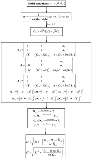
Figure A1.
Flowchart of calculating the error amplification factors.
References
- Takanashi, K.; Udagawa, K.; Seki, M.; Okada, T.; Tanaka, H. Nonlinear Earthquake Response Analysis of Structures by a Computer-Actuator On-Line System; University of Tokyo: Tokyo, Japan, 1975. [Google Scholar]
- Abbiati, G.; Bursi, O.S.; Caperan, P.; Di Sarno, L.; Molina, F.J.; Paolacci, F.; Pegon, P. Hybrid simulations of a multi-span RC viaduct with plain bars and sliding bearings. Earthq. Eng. Struct. Dyn. 2015, 44, 2221–2240. [Google Scholar] [CrossRef]
- Elnashai, A.S.; Di Sarno, L. Fundamentals of Earthquake Engineering; Wiley and Sons: Chichester, UK 2008. [Google Scholar]
- Chang, S.Y. Explicit pseudodynamic algorithm with unconditional stability. J. Eng. Mech. 2002, 128, 935–947. [Google Scholar] [CrossRef]
- Chen, C.; Ricles, J.M. Development of direct integration algorithms for structural dynamics using discrete control theory. J. Eng. Mech. 2008, 134, 676–683. [Google Scholar] [CrossRef]
- Kolay, C.; Ricles, J.M. Development of a family of unconditionally stable explicit direct integration algorithms with controllable numerical energy dissipation. Earthq. Eng. Struct. Dyn. 2014, 43, 1361–1380. [Google Scholar] [CrossRef]
- Kolay, C.; Ricles, J.M. Assessment of explicit and semi-explicit classes of model-based algorithms for direct integration in structural dynamics. Int. J. Numer. Methods Eng. 2016, 107, 49–73. [Google Scholar] [CrossRef]
- Peek, R.; Yi, W.H. Error analysis for pseudodynamic test method. I: Analysis. J. Eng. Mech. 1990, 116, 1618–1637. [Google Scholar] [CrossRef]
- Peek, R.; Yi, W.H. Error analysis for pseudodynamic test method. II: Application. J. Eng. Mech. 1990, 116, 1638–1658. [Google Scholar] [CrossRef]
- Shing, P.B.; Mahin, S.A. Cumulative experimental errors in pseudodynamic tests. Earthq. Eng. Struct. Dyn. 1987, 15, 409–424. [Google Scholar] [CrossRef]
- Shing, P.B.; Mahin, S.A. Experimental error effects in pseudodynamic testing. J. Eng. Mech. 1990, 116, 805–821. [Google Scholar] [CrossRef]
- Shing, P.B.; Manivannan, T. On the accuracy of an implicit algorithm for pseudodynamic tests. Earthq. Eng. Struct. Dyn. 1990, 19, 631–651. [Google Scholar] [CrossRef]
- Chang, S.Y. Nonlinear error propagation analysis for explicit pseudodynamic algorithm. J. Eng. Mech. 2003, 129, 841–850. [Google Scholar] [CrossRef]
- Chang, S.Y. Error propagation of HHT-α method for pseudodynamic tests. J. Earthq. Eng. 2005, 9, 223–246. [Google Scholar] [CrossRef]
- Chang, S.Y. Error propagation in implicit pseudodynamic testing of nonlinear systems. J. Eng. Mech. 2005, 131, 1257–1269. [Google Scholar] [CrossRef]
- Bousias, S.; Sextos, A.; Kwon, O.H.; Taskari, O.; Elnashai, A.S.; Evangeliou, N.; Di Sarno, L. Intercontinental hybrid simulation for the assessment of a three-span R/C highway overpass. J. Earthq. Eng. 2017. [Google Scholar] [CrossRef]
- Fu, B. Substructure Shaking Table Testing Method Using Model-Based Integration Algorithms. Ph.D. Thesis, Tongji University, Shanghai, China, 2017. (In Chinese). [Google Scholar]
- MATLAB. Version 2014a; The MathWorks Inc.: Natick, MA, USA, 2014.
- Chopra, A.K. Dynamic of Structures: Theory and Applications to Earthquake Engineering, 4th ed.; Prentice Hall: Upper Saddle River, NJ, USA, 2012. [Google Scholar]
- Chang, S.Y. The γ-function pseudodymamic algorithm. J. Earthq. Eng. 2000, 4, 303–320. [Google Scholar] [CrossRef]
© 2018 by the authors. Licensee MDPI, Basel, Switzerland. This article is an open access article distributed under the terms and conditions of the Creative Commons Attribution (CC BY) license (http://creativecommons.org/licenses/by/4.0/).