A Comprehensive Assessment and Spatial Analysis of Vulnerability of China’s Provincial Economies

Abstract

Vulnerability theory is a fundamental scientific knowledge system in sustainable development, and vulnerability assessment is important in vulnerability studies. Economic vulnerability affects economic growth sustainability. Comprehensive assessment of economic vulnerability in the process of economic growth under the theoretical framework of vulnerability will provide a new perspective for vulnerability studies. Based on a vulnerability scoping diagram assessment model, this study selected 22 economic sensitivity indexes and 25 economic adaptability indexes from the economic, social, and nature–resource–environmental subsystems to comprehensively assess and spatially analyse the vulnerability of China’s provincial economies since the year 2000, while applying the entropy method, multilevel extension assessment, spatial measurement method, and geographic information system technology. The results showed the following: (1) There are great differences in the vulnerability of China’s provincial economies. Western China’s vulnerability is higher and the fluctuation range of economic vulnerability is larger. The vulnerability increased significantly based on spatial differential features; (2) Regional differences in economic vulnerability, mainly caused by differences within a region, increased gradually. Eastern and Western China showed the spatial pattern characteristics of prominent and reinforcing regional imbalance, while Central and Northeast China showed declining regional imbalance. The spatial structure evolution of economic vulnerability is characterized by a volatility curve, and regional separation and divergence are strengthened; (3) Growth of China’s provincial economies and economic vulnerability are related negatively. In Eastern, Central, and Northeast China, vulnerability of the provincial economies has a negative spillover effect on neighbouring provinces’ economic growth, while in Western China it has a slight positive spillover effect.

1. Introduction

Vulnerability studies are mainly confined to geosciences. As vulnerability research is constantly being enriched, its scope has expanded to include natural disaster vulnerability, ecosystem vulnerability, groundwater system vulnerability, regional development system vulnerability, social vulnerability, and poverty vulnerability [1]. Multiple academic disciplines, such as geography, economics, ecology, sociology, management science, engineering science, and political science, have become the top concerns of vulnerability studies [2]. In 2001, Science listed vulnerability studies as one of seven core issues in sustainability science [3]. Vulnerability studies have become an important scientific approach to probe into the human–earth interaction mechanism in contemporary geography and relevant disciplines, as well as major cutting-edge scientific problems [4]. Vulnerability studies are now considered a fundamental system of scientific knowledge aiming to analyse the degree, mechanism, and process of human–earth interaction, as well as regional sustainable development [5]. The initial objective of vulnerability studies was examining the natural ecological environment system, but now it has expanded to include human system studies [6,7]. The concept connotations of vulnerability have expanded from the study of endogenous risk factors—which was based on natural vulnerability in the earlier days—into a multidimensional comprehensive category that integrates natural, economic, social, human, environmental, organizational, and institutional characteristics. The concept of vulnerability initially began as a dual structure of sensitivity and coping capability, but it has expanded into a multi-structured, conceptual collection of multiple elements, including sensitivity, coping capability, degree of exposure, and adaptability [8].

As the main content of vulnerability studies, economic vulnerability involves the expansion and utilization of vulnerability in the economic field. In 1990, the concept of economic vulnerability was first proposed at the United Nations Conference on Trade and Development held in Malta [9]. Economic vulnerability—first seen as an issue of sustainable economic development in least developed countries in the political–economic context—generally refers to uncontrollable exposure of an economic force due to its reliance on export, resulting from a shortage of natural resources, economic notarisation, and enclosed economic geography, which may cause difficulties in diversifying economic development, resulting in economic crises or economic risks [10]. In 1999, the United Nations Development Program officially defined economic vulnerability as tolerance of an economy towards damage caused by unexpected shocks in the process of economic development [11]. Briguglio believes that economic vulnerability is as an essential attribute of an internal system, and the economic vulnerability of countries with higher gross domestic product per capita is accordingly higher; the author thus came up with the “Singapore Paradox” regarding economic vulnerability [12]. Some scholars hold that economic vulnerability is similar to risk [13], and economic risk is closely related to economic vulnerability and economic resilience. Economic risk may cause direct economic losses, while economic vulnerability, as an essential attribute of the system, will magnify such impact and response in times of external shocks. Economic resilience denotes the competence scope within which the welfare loss is reduced in times of external shocks, and it sometimes signifies the recovery capability of an economy after its exposure to external risk. Briguglio et al., summarizes economic risk, economic vulnerability, and economic resilience with an equation; economic risk is the result when economic resilience is subtracted from economic vulnerability [12,14,15,16,17,18,19].Yet, most scholars define economic vulnerability from the perspective of an economic system, and maintain that the vulnerability of an economic system refers to its essential attribute that may expose the system to harm due to the economic system’s sensitivity during internal and external disturbances and lack of capability to deal with unfavorable disturbances [12,14,20,21,22]. Some scholars think of economic vulnerability as uncertainty in the macro-economic or regional economic system [23,24]. From the perspective of economic growth and existing research literature, this study suggests that economic vulnerability is an essential attribute of the system in the process of economic growth and that it may cause potential loss of economic growth, thus affecting sustainable economic growth. Economic vulnerability manifests as two aspects—economic sensitivity and economic adaptability—which can be presented as measurable functional relationships [25,26].

Economic vulnerability has an impact on the sustainability of economic growth. In the 1990s, after China reformed the economic system based on the market economy, the system was prone to external shocks and disturbances caused by economic globalization. This led to vulnerability that affected the macro-economic growth, such as the Asian financial crisis (1997) and global financial crisis (2008). There are some “black swans” lurking in many aspects of China’s economic growth, such as real estate investment, industrial transformation and development, financial venture, urbanization, resident income, social security, environmental investment, and governance [27]. Each black swan is a “window of opportunity” in China’s economic growth, although it may simultaneously bring a potential negative effect to economic growth, which will cause loss of economic growth, leading to downward or stagnant economic growth and thus higher economic vulnerability. After 2010, a significant slowdown in China’s economic growth indicates that China entered an era of the “three periods superimposed”, which consists of the three periods of change of pace in economic growth, economic structural adjustment, and digestion of economic stimulus policy. Thus, China’s economic growth faced more uncertainty [28]. In 2015, the vulnerability of China’s economy became one of two main themes of the world economy [29], causing great worldwide concern for the sustainability of China’s economic development. As for economic vulnerability studies, Chinese scholars pay more attention to the urban-type (resources-based city [20,22,30,31,32], coastal city [24,33,34,35,36], tourist city [37,38], etc.) economic vulnerability and sustainable development issues in urban areas, and there are few studies that deal with economic vulnerability in the process of economic growth. The economic growth of different provinces in China is characterized by difference and imbalance. The economic aggregate of Eastern China takes up a larger share and Western China needs to catch up with Eastern China in terms of economic speed. Yet if there is some blind pursuit of speed of economic growth on the part of Western China, the system of economic growth is bound to be disturbed by external shocks and impacts. Thus a lack of adaptability in some areas will inevitably cause greater economic vulnerability and even uncertain economic risk. In the process of market-oriented reforms, the economic growth in different provinces in China is confronted with various shocks and impacts, and some structural conflicts are difficult to solve in a short period of time, therefore distinctive characteristic of vulnerability can see in economic growth [21,24,26,39,40].

Currently, economic vulnerability studies are generally carried out under the framework of vulnerability studies, and there are few studies dedicated to constructing a theoretical framework for economic vulnerability studies. Due to different research perspectives of economic vulnerability, scholars find it difficult to reach a consensus regarding the concept of economic vulnerability. Adger believes that the concept of vulnerability is difficult to define accurately, but it can be measured [41], and the assessment and measurement of vulnerability is an important part and main direction of vulnerability studies. Current economic vulnerability studies are mainly focused on state assessment and counter measures, with an emphasis on the summarization of vulnerability in a general sense, while the study of rules and processes of the spatial evolution of vulnerability is inadequate and economic vulnerability studies in different geospatial scales are scarce. The assessment index system and assessment methods in current literature do not fully apply to the economic vulnerability assessment of China’s economic growth, due to the lack of a scientific assessment from the perspective of a multi-scale system, and the neglect of economic growth as a substantive characteristic of interrelated systems in terms of assessment method [2,12,13,14,30,31,32,42,43]. This article makes further endeavours on the research index and assessment method, and takes sustainable economic growth as its research perspective. It is believed that economic growth is a compound system that consists of economic subsystems, social subsystems, and nature–resource–environmental subsystems. With the establishment of a vulnerability assessment index system, a comprehensive assessment will be conducted using the multilevel extension assessment method. Therefore, from the perspective of economic growth sustainability, the aim of this article is to contribute to constructing a comprehensive assessment index system for economic vulnerability; conduct a comprehensive assessment of economic vulnerability at the provincial level; clarify the basic situation of vulnerability of China’s provincial economies and the evolution patterns of its spatial structure; and explore the spatially interactive relations between economic vulnerability and economic growth, with the aim of providing a scientific decision-making basis for ordering the transformation of national and provincial promotion of economic growth in the spatial structure, as well as proving a path and direction of space governance to help reduce and cope with economic vulnerability to achieve sustainable economic growth.

This article is organised as follows: Section 2 outlines the methodology of Economic vulnerability. Section 3 then analyses of assessment results of vulnerability. After presenting spatial analysis in Section 4, Section 5 draws a conclusion and discusses the findings.

2. Methodology

2.1. Assessment Model of Economic Vulnerability

Based on existing literature about vulnerability [44,45,46,47,48], there are mainly three function models of vulnerability: respectively, the VSD Model (Vulnerability Scoping Diagram) [44,45,46], VSR Model (V-vulnerability, S-exposure-sensitivity, R-response capacity) [38], and PSE Model (P-pressure, S-sensitivity, E-elasticity) [47,48]. The VSD Model is a basic functional form that can better illustrate the essential attributes of vulnerability studies. Therefore, this study uses a VSD model for assessing economic vulnerability. Its functional form is as follows:

$$V_i=\frac{S_i}{D_i}$$

(1)

Here, $V_i$ is the economic vulnerability of a system (or region) $i$; $S_i$ is the economic sensitivity of system (or region) $i$; $D_i$ is the economic adaptability of system(or region) $i$.

Previous literature interprets the VSD model as a positive functional relation between economic vulnerability and economic sensitivity: the greater is the sensitivity caused by the disturbance, the greater is the vulnerability. Moreover, there is a negative functional relation between adaptability and vulnerability: the greater the adaptability, the smaller the vulnerability [44,45,46]. After reviewing the related literature, this paper argues that economic sensitivity is the mechanism of interactions among economic subsystems, social subsystems, and nature–resource–environmental subsystems in the process of sustainable economic development, which is characterized by the degree of impact and response of each subsystem to internal and external factor changes; thus, it is a function of economic vulnerability [8,9,49,50,51]. Economic adaptability is the self-adaptive process of each subsystem when internal and external environment changes take place in the process of sustainable economic development, which is manifested as an adaptive capacity that forms a certain functional relation with economic vulnerability and an effective decision-making system that can adjust, manage, and plan sustainable economic development [12,14,15,16,17,18,19,42,51,52]. The VSD model of economic vulnerability can be interpreted as follows: there is a functional relationship between economic vulnerability, economic sensitivity, and economic adaptability. Economic vulnerability is determined by economic sensitivity, which is generated when the system is affected by disturbances and economic adaptability of the system’s self-organization. When economic sensitivity is strong and economic adaptability of the system’s self-organization is weak, economic vulnerability will increase. On the contrary, when economic sensitivity is weak and economic adaptability of the system self-organization is strong, economic vulnerability will decrease [21,22,23,44,45,46].

2.2. Comprehensive Assessment Index System of Economic Vulnerability

According to the VSD Model, the construction of the index system of economic vulnerability involves economic sensitivity indexes and economic adaptability indexes. With regard to indicator selection, this paper observes the principles of scientificity, systematization, dynamicity, dominance, universality, and operability. As for data information obtainment, this paper takes into full account the accessibility and reliability of indicator data and tries its best to avoid the impact of human factors to deliver quantification and spatialization expressions to ensure the accuracy, scientificity, and objectivity of vulnerability assessment results. There is some related literature [2,12,14,21,22,23,25,26,44,45,46,47,48,49,50,51,52,53,54,55,56,57]. A multi-dimensional perspective involving the economic subsystems, social subsystems, and nature–resource–environmental subsystems will be conducive to the establishment of economic vulnerability index systems. There are different levels and indexes for each subsystem, each of which is not only correlated with in-system indexes, but also correlated with various levels and indexes of other systems to some extent. There are 17 third-class indexes and 22 four-class indexes of economic sensitivity, including 11 four-class indexes of the economic subsystem, 6 four-class indexes of the social subsystem, and 5 four-class indexes of the nature–resource–environmental subsystem (

Table 1. Index system for economic sensitivity.

First-Class Index	Second-Class Index	Third-Class Index	Fourth-Class Index	Unit	Weight
economic sensitivity	economic subsystem	economic fluctuation	fluctuation range of economic growth (S1)	-	0.0595
		industrial disturbance	disturbance degree of primary industry (S2)	-	0.0473
			disturbance degree of secondary industry (S3)	-	0.0424
			disturbance degree of tertiary industry (S4)	-	0.0465
		investment disturbance	disturbance degree of investment (S5)	-	0.0417
		consumption change	urban–rural consumption ratio (S6)	-	0.0167
		trade pressure	foreign trade dependence degree (S7)	%	0.0382
		financial risk	fluctuation range of exchange rate (S8)	Ұ/1 $	0.0256
			loan–deposit ratio (S9)	-	0.3626
		fiscal risk	financial deficit ratio (S10)	%	0.0115
		price fluctuation	absolute value of inflation rate (S11)	%	0.0209
	social subsystem	rural-urban divide	urban–rural income ratio (S12)	-	0.0234
		gap between the rich and the poor	Gini coefficient (S13)	-	0.0128
		employment influence	registered urban unemployment rate (S14)	%	0.0214
		poverty pressure	poverty incidence in rural areas (S15)	%	0.0370
		educational influence	dropout rate of school-age children (S16)	%	0.0119
		resident health	annual hospitalization rate of residents (S17)	%	0.0396
	nature–resource–environmental subsystem	natural disasters	growth rate of direct economic loss caused by natural disasters (S18)	%	0.0429
		energy consumption	elastic coefficient of energy consumption (S19)	-	0.0263
		environmental pollution	Growth rate of discharge amount of industrial waste water (S20)	%	0.0216
			Growth rate of discharge amount of industrial waste gas (S21)	%	0.0172
			Growth rate of discharge amount of industrial solid wastes (S22)	%	0.0332

). There are 9 third-class indexes and 25 four-class indexes of economic adaptability, including 12 four-class of the economic subsystem, 6 four-class of the social subsystem, and 7 four-class of the nature–resource–environmental subsystem (

Table 2. Index system for economic adaptability.

First-Class Index	Second-Class Index	Third-Class Index	Fourth-Class Index	Unit	Weight
economic adaptability	economic subsystem	economic efficiency	capital productivity (D1)	-	0.0506
			labor productivity (D2)	Ұ/person	0.0501
			total factor productivity (D3)	-	0.0134
		economic institution	non-fiscal expenditure in GDP (D4)	%	0.0328
			percentage of non-state-owned economy in total industrial output value (D5)	%	0.0188
			percentage of foreign investment in actual use in GDP (D6)	%	0.0406
			patent authorizations per 10,000 persons (D7)	patent/10,000 persons	0.1162
			Percentage of R&D expenditure in GDP (D8)	%	0.0365
		economic development	GDP per person (D9)	Ұ	0.0495
			percentage of industrial added value in GDP (D10)	%	0.0159
			percentage of added value of tertiary industry in GDP (D11)	%	0.0299
			percentage of household consumption expenditure in GDP (D12)	%	0.0477
	social subsystem	social development	urbanization rate (D13)	%	0.0539
		social security	percentage of people with unemployment insurance in people in employment (D14)	%	0.0408
			percentage of people with basic endowment insurance in total population (D15)	%	0.1347
			coverage of community service institutions (D16)	%	0.0230
		social investment	percentage of educational expenditure in GDP (D17)	%	0.0304
			percentage of total health expenditure in GDP (D18)	%	0.0191
	nature–resource–environmental subsystem	prevention of natural disasters	natural disaster relief per 10,000 persons (D19)	Ұ10,000/10,000 persons	0.0727
		energy production	elastic coefficient of energy production (D20)	-	0.0094
			overall efficiency of energy processing and transforming (D21)	%	0.0102
		Environmental improvement	percentage of investment in treatment of industrial pollution in total industrial output value (D22)	%	0.0230
			standard-meeting rate of industrial waste water discharge (D23)	%	0.0295
			standard-meeting rate of industrial sulphur dioxide (D24)	%	0.0238
			overall utilization of industrial solid wastes (D25)	%	0.0275

).

Most index data are collected as statistical data from yearbooks, while some calculation data are acquired in strict accordance with the theoretical equations in index descriptions (See Appendix A and Appendix B). Due to insufficient data about economic vulnerability of the Hong Kong Special Administrative Region, Macao Special Administrative Region, and Taiwan province, these three regions are not included in this study. The entropy method uses the utility value of information of indexes to determine the weight of an index, which avoids the impact of subjective factors on index weights [58,59].

2.3. Assessment Method of Economic Vulnerability

2.3.1. Multilevel Extension Assessment Method

This study adopts the multilevel extension assessment method to conduct a comprehensive assessment of economic vulnerability. Introduced by Cai in 1983, the extenics theory adopts formalised models to assess the applicability of extenics as well as the laws and methods of innovation. Extenics theory describes three elements, which are the matter, character, and corresponding character value. These elements are assumed to solve contradictory and incompatible problems qualitatively and quantitatively [60,61,62,63,64]. The multilevel extension assessment is the expression of matter-element with triple $R=(U,C,V)$. If matter U has n characteristics $C(c_1,c_2,\cdots ,c_n)$, m matter-element to be assessed $R_1=(U_1,C,V_1),R_2=(U_2,C,V_2),\cdots ,R_m=(U_m,C,V_m)$ has the same characteristic C, then matter-element R with the same characteristic can be expressed as

$$R=\left[\begin{array}{ccccc}U& U_1& U_2& \cdots & U_m\\ c_1& v_{11}& v_{12}& \cdots & v_{1m}\\ c_2& v_{21}& v_{22}& \cdots & v_{2m}\\ \begin{array}{l}⋮\end{array}& \begin{array}{l}⋮\end{array}& \begin{array}{l}⋮\end{array}& \begin{array}{l}⋮\end{array}& \begin{array}{l}⋮\end{array}\\ c_n& v_{n1}& v_{n2}& \cdots & v_{nm}\end{array}\right]$$

(2)

In this equation, $U_m$—matter-element to be assessed; $U$—the whole body of matter-element to be assessed $U_1,U_2,\cdots ,U_m$; $v_{ij}$—value of the $i$th characteristic of the $j$th matter-element to be assessed, $i=1,2,\cdots ,n$; $j=1,2,\cdots ,m$.

Suppose there is m matter-element to be assessed (or category of assessment) $U_1,U_2,\cdots ,U_m$, using $[a_{ij},b_{ij}]$ to indicate the range of characteristic value of matter-element (or category) to be assessed, then matter-element with the same characteristic $R$ can be expressed as

$$R=\left[\begin{array}{ccccc}U& U_1& U_2& \cdots & U_m\\ c_1& [a_{11},b_{11}]& [a_{12},b_{12}]& \cdots & [a_{1m},b_{1m}]\\ c_2& [a_{21},b_{21}]& [a_{22},b_{22}]& \cdots & [a_{2m},b_{2m}]\\ \begin{array}{l}⋮\end{array}& \begin{array}{l}⋮\end{array}& \begin{array}{l}⋮\end{array}& \begin{array}{l}⋮\end{array}& \begin{array}{l}⋮\end{array}\\ c_n& [a_{n1},b_{n1}]& [a_{n2},b_{n2}]& \cdots & [a_{nm},b_{nm}]\end{array}\right]$$

(3)

In this equation, $U_m$—the $j$th matter-element (or category) to be assessed; $c_i$—the $i$th evaluation index; $v_{ij}=[a_{ij},b_{ij}]$—the value range of $c_i$ defined by defined by $U_j$ $U_j$, that is, the classical domain.

Based on this, the Multilevel Extension Assessment Method will be established. By identifying matter-elements with the same characteristics, determining the value range of every characteristic, describing the characteristic values of matter-element to be assessed and calculating correlation degrees, the category to which the matter-element to be assessed belongs will be finally concluded [60,61,62,63,64].

The extenics method has been applied in the literature as an assessment tool [63,64]. As this method not only qualitatively analyses the state of being of the system during the market-oriented process but also quantitatively analyses the adaptation capacity of the system and the changes that occur at different stages, this research adopts the extenics method to assess economic growth adaptation for the first time.

The multilevel extension assessment method is divided into the following steps [60,61,62,63,64]:

Step one: Identify grade theory domain U and assessment factor set C. First, set the domain name as follows:

$$U=\{U_j,j=1,2,\cdots ,m\}$$

(4)

of which the grade theory domain is divided into $j$ assessment grades. Then, set assessment index factor set as follows:

$$C=\{c_i,i=1,2,\cdots ,m\}$$

(5)

of which $i$ is the number of assessment indexes.

Step two: Identify classical domain and joint domain. Suppose,

$$R_j=(U_j,C,V_j)=\left[\begin{array}{ccc}{U}_j& c_1& \langle a_{j1},b_{j1}\rangle \\ & c_2& \langle a_{j2,}{b}_{j2}\rangle \\ & \cdots & \cdots \\ & c_n& \langle a_{jm},b_{jn}\rangle \end{array}\right]$$

(6)

In this equation, $V_j$ is the classical domain of $U_j$, which serves as the range value in the assessment index set C chosen according to grade $U_j$. $a_{jm}$ represents the matrix of lower limit of classical domain, and $b_{jn}$ represents the matrix of upper limit of the classical domain.

Suppose,

$$R_U=(U,C,V_U)=\left[\begin{array}{ccc}U& c_1& \langle a_{U1},b_{U1}\rangle \\ & c_2& \langle a_{U2,}{b}_{U2}\rangle \\ & \cdots & \cdots \\ & c_n& \langle a_{Um},b_{Un}\rangle \end{array}\right]$$

(7)

In this equation, $V_U$ is the joint domain, which serves as the range value in the assessment index set C chosen according to grade U. $a_{Um}$ is the matrix of lower limit of joint domain, and $b_{Un}$ is the matrix of upper limit of joint domain.

Step three: Identify the assessment matter-element. The formula of the matter-element assessment is

$$R_i==\left[\begin{array}{ccc}N& c_{ik}& v_{i1}\\ & c_{i2}& v_{i2}\\ & \cdots & \cdots \\ & c_{ik}& v_{ik}\end{array}\right]$$

(8)

In this equation, N is the assessment object; $v_{ik}$ is the value of $c_{ik}$ associated with assessment object N; $k=1,2,\cdots ,p$, $p$ is the number of secondary index.

Step four: Calculate the correlation degree of index. The degree of correlation of second-class index is

$$k_j(c_{ik})=\{\begin{array}{cc}\frac{\rho (v_{ik},V_j)}{\rho (v_{ik},V_U)-\rho (v_{ik},V_j)},& x\notin (a_{kj}^i,b_{kj}^i)\\ 0.05& v_{ik}=a_{kj}^{i}or{v}_{ik}=b_{kj}^i\\ \frac{\rho (v_{ik},V_j)}{b_{kj}^i-a_{kj}^i},& x\in (a_{kj}^i,b_{kj}^i)\end{array}$$

(9)

$k_j(c_{ik})$ is the degree of correlation of grade j in second-class index K in order within the first-class index. The correlation coefficient is in the formula i

$$\rho (v_{ik},V_j)=\left|v_{ik}-\frac{a_{ji}+b_{ji}}{2}\right|-\frac{(b_{ji}-a_{ji})}{2}$$

(10)

$$\rho (v_{ik},V_U)=\left|v_{ik}-\frac{a_{Ui}+b_{Ui}}{2}\right|-\frac{(b_{Ui}-a_{Ui})}{2}$$

(11)

Multiplying the weight vector of the second-class index by the correlation degree matrix of different grades of second-class index, we calculate the correlation degree matrix of first-class index as follows:

$$k(c_i)=(k_j(c_i))=\left[w_{i1},w_{i2},\cdots ,w_{ip}\right]•\left[\begin{array}{cccc}{k}_1(c_{i1})& k_2(c_{i1})& \cdots & k_m(c_{i1})\\ k_1(c_{i2})& k_2(c_{i2})& \cdots & k_m(c_{i2})\\ \cdots & \cdots & \cdots & \cdots \\ k_1(c_{ip})& k_2(c_{ip})& \cdots & k_1(c_{ip})\end{array}\right]$$

(12)

Multiplying the weight vector of the first-class index by first-class correlation coefficient, we calculate the correlation coefficient matrix of assessment object as follows:

$$k(N)=\left[w_1,w_2,\cdots ,w_n\right]•\left[\begin{array}{cccc}{k}_1(c_1)& k_2(c_1)& \cdots & k_m(c_1)\\ k_1(c_2)& k_2(c_2)& \cdots & k_m(c_2)\\ \cdots & \cdots & \cdots & \cdots \\ k_1(c_n)& k_2(c_n)& \cdots & k_1(c_n)\end{array}\right]$$

(13)

Step five: Assessment results. Determine assessment grade as follows: if $k_{j0}(N)=\underset{j=\{1,2,\cdots ,m\}}{\max }{k}_j(N)$, then the assessment object N belongs to grade $j$.

The assessment coefficient is

$$j^{\ast }=\frac{{\displaystyle \sum _{j=1}^{m}j\cdot k_j^{\prime }(N)}}{{\displaystyle \sum _{j=1}^m{k}_j^{\prime }(N)}}$$

(14)

of which $k_j^{\prime }(N)=\frac{k_j(N)-\underset{j}{\min } k_j(N)}{\underset{j}{\max } k_j(N)-\underset{j}{\min } k_j(N)}$, and $j^{\ast }$ is the grading coefficient.

2.3.2. Explanations about the Multilevel Extension Assessment Method of Economic Vulnerability

Set grade theory domain. The grade theory domain of economic sensitivity is as follows: $U_s=\{U_{1s},U_{2s},U_{3s}\}$ = {weak sensitivity, medium sensitivity, and strong sensitivity}. When the disturbance and impact on economic growth are not strong, weak sensitivity occurs; when they are apparent and the system is within a reasonable threshold, medium sensitivity occurs; when they are huge and the system is unstable, strong sensitivity occurs. The stronger the sensitivity, the higher the vulnerability.

Grade theory domain of economic adaptability is as follows: $U_D=\{U_{1D},U_{2D},U_{3D}\}$ = {low adaptability, medium adaptability, and high adaptability}. Low adaptability occurs when the adaptive capacity hinders or restricts sustainable economic development; medium adaptability indicates that demand of sustainable growth is basically met. High adaptability indicates that the current demand of economic growth is met, and economic growth will be promoted for some time in the future. Higher adaptability is conducive to economic sustainable growth, and vulnerability will be reduced in the meantime.

Set assessment factor set. The assessment factor set of economic sensitivity is as follows:

$$C_s=\{c_{si},i=1,2,\cdots ,m\}$$

(15)

of which $c_{si}$ is the four-class index of economic sensitivity and $i$ is the number of indexes. The assessment factor set of economic adaptability is thus as follows:

$$C_D=\{c_{Dj},j=1,2,\cdots ,n\}$$

(16)

of which $c_{Di}$ is the four-class index of economic adaptability, and n is the number of indexes.

Identify classical domain and joint domain. Classical domain and joint domain are mainly identified according to the corresponding range value of index data. There are three different levels of standard-setting principles for economic sensitivity and economic adaptability: national standards, theoretical perspectives, and expert opinions. The standard-setting principles are as follows: for data that meet international standards, international warning line is the minimum standard; standards found in relevant literature will be seen as theoretical perspectives; for data that are not related to any international warning line or theoretical perspective, expert opinions will be taken into account.

Determine the weight of indexes. This paper applies the entropy method in Shannon C E and Weaver W (1947) to determine the Weight of indexes [58,59].

Type classification of economic vulnerability. Based on classification standards of grade theory domain in the process of economic sensitivity and economic adaptability assessments, economic vulnerability is divided into nine different types as seen in

Table 3. Types for the comprehensive assessment of economic vulnerability.

Type	Number of the Type
high sensitivity–low adaptability	1
high sensitivity–medium adaptability	2
high sensitivity–high adaptability	3
medium sensitivity–low adaptability	4
medium sensitivity–medium adaptability	5
medium sensitivity–high adaptability	6
weak sensitivity–low adaptability	7
weak sensitivity–medium adaptability	8
weak sensitivity–high adaptability	9

.

2.4. Analysis Method of Regional Differences

This study uses the Theil index to conduct the spatial structure analysis of regional differences of economic vulnerability. The formula of the Theil index is as follows [65]:

$$T(V)=T_{BR(V)}+T_{WR(V)}={\displaystyle \sum _{i=1}^4{V}_i}\cdot \log \left(\frac{V_i}{Y_i}\right)+{\displaystyle \sum _{i=1}^4{V}_i}\times \left[{\displaystyle \sum _{j=1}{V}_{ij}}\cdot \log \left(\frac{V_{ij}}{Y_{ij}}\right)\right]$$

(17)

of which $T(V)$ is the overall difference in vulnerability between China’s provincial economies; $T_{BR(V)}$ is the intraregional economic vulnerability difference; $i$ is the economic region (according to the classification standards established by the National Bureau of Statistics of China, there are four economic regions: Eastern, Central, Western, and Northeast.); $V_i$ is the proportion of the economic vulnerability of a province in economic region $i$ in the economic vulnerability of 31 provinces in China; $Y_i$ is the proportion of GDP of all provinces in economic region $i$ in China’s economic aggregate; $V_{ij}$ is the proportion of economic vulnerability of province $j$ in economic region $i$ in the total sum of economic vulnerability of all provinces in economic region $i$; $Y_{ij}$ is the proportion of economic aggregate of province $j$ in economic region $i$ in the total sum of economic aggregate of all provinces in economic region $i$.

A greater $T(V)$ indicates greater difference in the economic vulnerability of different provinces in China. A greater $T_{BR(V)}$ indicates greater difference in economic vulnerability of different economic regions. A greater $T_{WR(V)}$ indicates greater difference in economic vulnerability of different provinces in an economic region.

When interregional and intraregional economic vulnerability affect the regional difference in overall economic vulnerability, this study uses the contribution rate for analysis. The formula of the contribution rate for interregional economic vulnerability is as follows:

$$W_{BR(V)}=\frac{T_{BR(V)}}{T(V)}\times 100\%$$

(18)

The formula of the contribution rate for intraregional economic vulnerability is as follows:

$$W_{WR(V)}=\frac{T_{WR(V)}}{T(V)}\times 100\%$$

(19)

In their study of the Theil index, O’Kelly and Pakes consider the manifestations of regional difference in different time periods and use the regional separation index to uncover the variability characteristics of regional spatial difference patterns [66]. The formula of the regional separation index is as follows:

$$S_{R(V)}=\frac{T_{BR(V)}}{\ln \left(\frac{Y}{Y_{\min }}\right)}\times \frac{\ln (Y_{\min })}{T_{WR(V)}}$$

(20)

of which $S_{R(V)}$ is the regional separation index of the economic vulnerability of a province in China; $Y$ is the total sum of economic aggregate of all provinces in China; $Y_{\min }$ is the economic aggregate of the province with the lowest economic aggregate in China.

2.5. Enactment of Spatial Econometric Model

Drawing on previous experience of experts who introduced some variables into the Cobb-Douglas (C-D) production function model, this study attempts to apply economic vulnerability as an independent factor to the production function model [67,68,69]. A correlation analysis of economic vulnerability and economic growth of different provinces in China from 2000 to 2014 indicates that the correlation coefficient R-square is 0.964, which is “highly correlated”, thus economic vulnerability has an obvious impact on economic growth and can be included in the C-D Model. The production function expression with the introduction of economic vulnerability model is as follows:

$$Y=A{K}^{\alpha }{L}^{\beta }{e}^{\lambda V}$$

(21)

in which $Y$ is the economic aggregate (GDP), $K$ is capital, $L$ is labour, $A$ is total factor productivity (technological level), $\alpha$ is the output elasticity of capital stock, $\beta$ is the output elasticity of labour stock, $\lambda$ is the influence coefficient of economic vulnerability on economic growth, and $V$ is economic vulnerability. Taking the log of both sides of Formula (21), and we get the linear transformation form that includes economic vulnerability:

$$\ln Y=\ln A+\alpha \ln K+\beta \ln L+\lambda V$$

(22)

The implications of this model are as follows: with the introduction of economic vulnerability, we can inquire into the change of technological levels, production factors input, and impact of economic vulnerability on economic growth.

Enactment of the spatial lag model (SLM). After the introduction of spatial independent variables, the SLM is as follows [42]:

$$\ln Y=\rho W\ln Y+\ln A+\alpha \ln K+\beta \ln L+\lambda V+\mu ,\mu ~N(0,{\sigma }^{2}I)$$

(23)

in which $\mu$ − ($n\times 1$) is the error term vector of order normal distribution, and $\rho$ is the spatial autoregressive coefficient. and W is the spatial weight. Since geographic proximity is easier to measure than geographical distance and economic distance, this paper mainly analyzes provincial spillover effect, and spatial econometrics of different provinces in China adopting proximal spatial weight matrix will be more appropriate [67,68,69].

Enactment of the spatial error model (SEM). After the introduction of spatial independent variables, the SEM is as follows [70]:

$$\ln Y=\ln A+\alpha \ln K+\beta \ln L+\lambda V+\gamma W\epsilon +\mu ,\mu ~N(0,{\sigma }^{2}I)$$

(24)

in which $\gamma$ is the vector coefficient of the correlation intensity of regression residual space, which can be used to measure the direction and degree of influence imposed by the economic growth of neighbouring regions on that of this region.

Enactment of the spatial durbin model (SDM). After introduction of the spatial independent variables, the SDM is as follows [71]:

$$\begin{array}{ll}\ln Y& =\rho W\ln Y+\ln A+\alpha \ln K+\beta \ln L+\lambda V\\ & +\gamma W\overline{(\ln A+\alpha \ln K+\beta \ln L+\lambda V)}+\gamma W\epsilon +\mu ,\mu ~N(0,{\sigma }^{2}I)\end{array}$$

(25)

in which $\overline{(\ln A+\alpha \ln K+\beta \ln L+\lambda V)}$ is the explanatory variable matrix of $n\times (Q-1)$, and $\gamma$ is the parameter vector of $n\times (Q-1)$, which can be used to measure the border effect of the economic growth of neighbouring provinces on this province. $\gamma W\overline{(\ln A+\alpha \ln K+\beta \ln L+\lambda V)}$ is the spatial lag explanatory variable of average observed value of neighbouring provinces.

2.6. Data Sources

In this article, data are obtained from China Statistical Yearbook for Regional Economy (2000–2015), Statistics Database of China’s Economic and Social Development, statistical yearbooks of 31 provinces and regions in China from 1999 to 2015, statistical data of China Yearbooks Full-text Database, of which some data are acquired in strict accordance with theoretical equations (see Appendix A and Appendix B). A spatial econometric analysis has been conducted according to panel data estimation from 2000 to 2014. With regard to spatial weight, we use the proximal spatial weight matrix to spatially measure every province in China. In this model, the data come from statistical yearbooks of different provinces from 2000 to 2014 in China. In the calculation formula in Appendix B, Y indicates GDP, L indicates employment, variable capital K indicates capital stock and total factor productivity (A), and economic vulnerability (V) is the calculation result of a comprehensive assessment of the vulnerability of China’s provincial economies from 2000 to 2014. Matlab10.0 is used to conduct calculations.

3. Overall Analysis of Assessment results of Economic Vulnerability

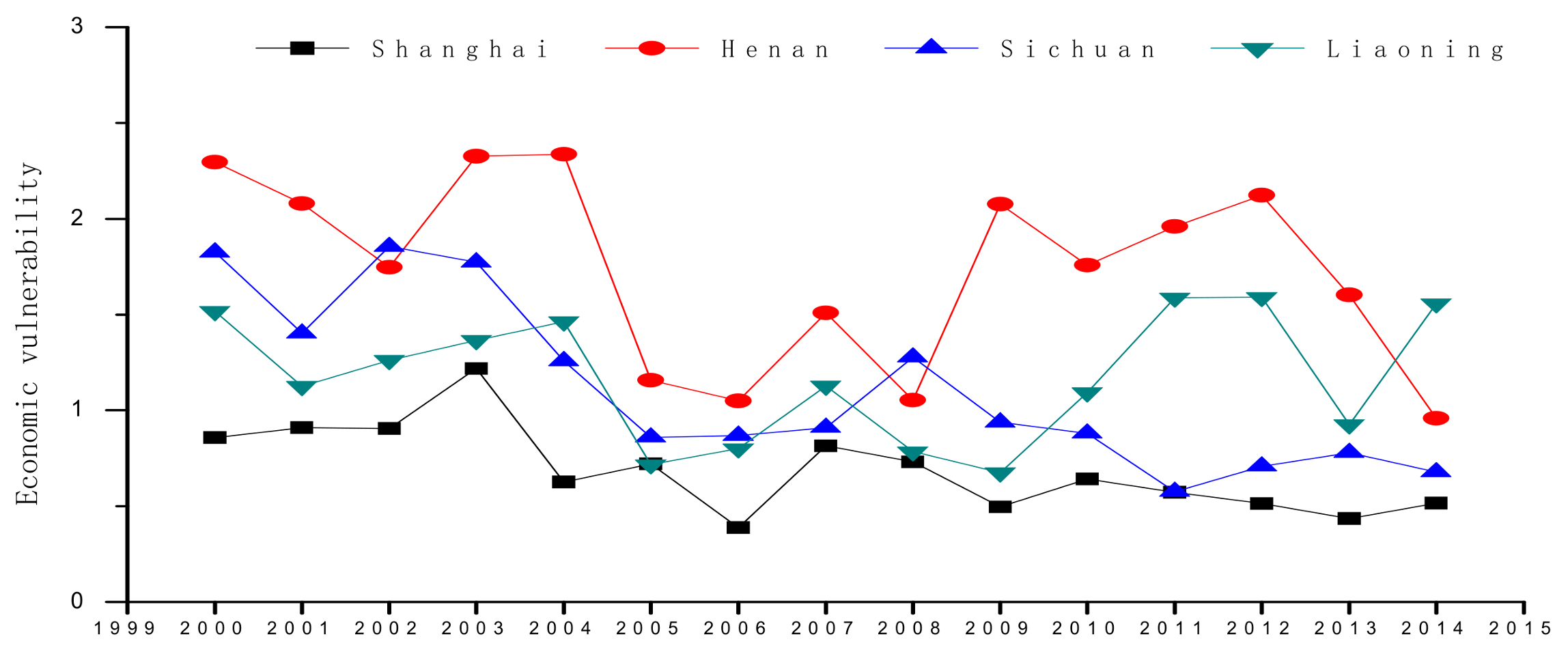
3.1. Economic Vulnerability and Ranking of China’s Provinces in Different Periods

In 2014, economic vulnerability was lowest in Guangdong (0.4354) and highest in Guangxi (1.8851). The economic vulnerability of Guangxi is 4.3 times as high as that of Guangdong. Provinces with higher economic vulnerability are mainly located in Western China, such as Guizhou, Qinghai, Ningxia, Inner Mongolia, Yunnan, and Guangxi, as well as Henan in Central China. Provinces with lower economic vulnerability are mainly located in Eastern China, including Shanghai, Beijing, Guangdong, Jiangsu, Zhejiang, and Tianjin, as well as Heilongjiang and Liaoning in Northeast China and Jiangxi in Central China. Significant variations can be seen in the vulnerability of China’s provincial economies (see Appendix C and

Table 4. The top and last five Chinese provinces based on economic vulnerability.

Period of Time	Five Provinces with Highest Average Economic Vulnerability (Ranking)	Five Provinces with Lowest Average Economic Vulnerability (Ranking)
2000–2004	Henan (1), Qinghai (2), Guizhou (3), Inner Mongolia (4), and Ningxia (5)	Shanghai (31), Beijing (30), Guangdong (29), Zhejiang (28), and Fujian (27)
2005–2009	Guizhou (1), Yunnan (2), Qinghai (3), Ningxia (4), and Inner Mongolia (5)	Shanghai (31), Beijing (30), Heilongjiang (29), Liaoning (28), and Tianjin (27)
2010–2014	Guangxi (1), Guizhou (2), Henan (3), Ningxia (4), and Qinghai (5)	Beijing (31), Shanghai (30), Guangdong (29), Jiangsu (28), and Jiangxi (27)
2000–2014	Guizhou (1), Qinghai (2), Ningxia (3), Inner Mongolia (4), and Henan (5)	Shanghai (31), Beijing (30), Guangdong (29), Jiangsu (28), and Jiangxi (27)

). There are obvious fluctuations in terms of economic vulnerability of different provinces from 2000 to 2014. Shanghai in Eastern China and Sichuan in Western China show the fluctuation tendency of gradual decrease, while the fluctuation tendency of economic vulnerability of Henan in Central China and Liaoning in Northeast China is not distinctive, and the fluctuation range is relatively large (Figure 1).

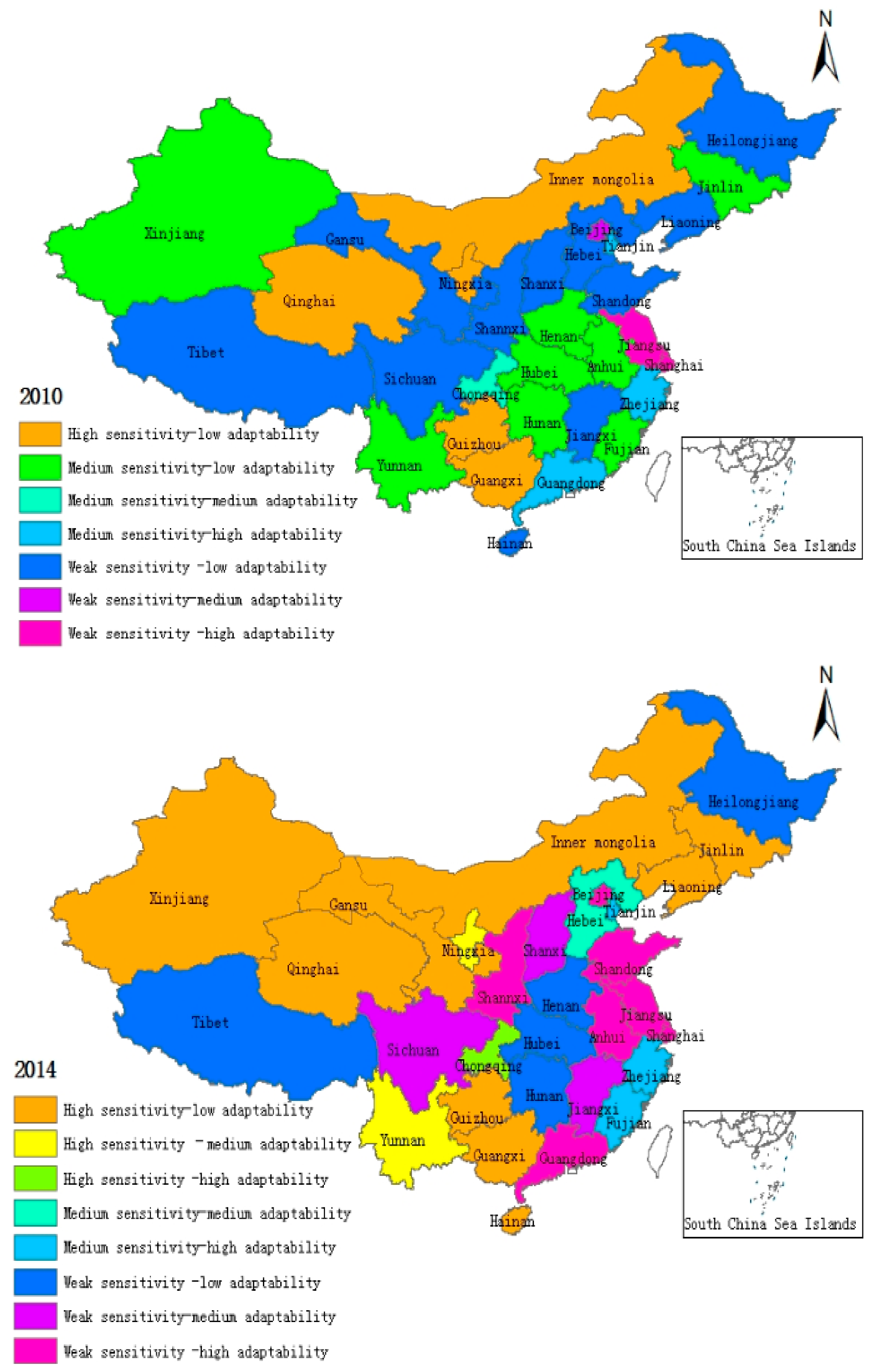
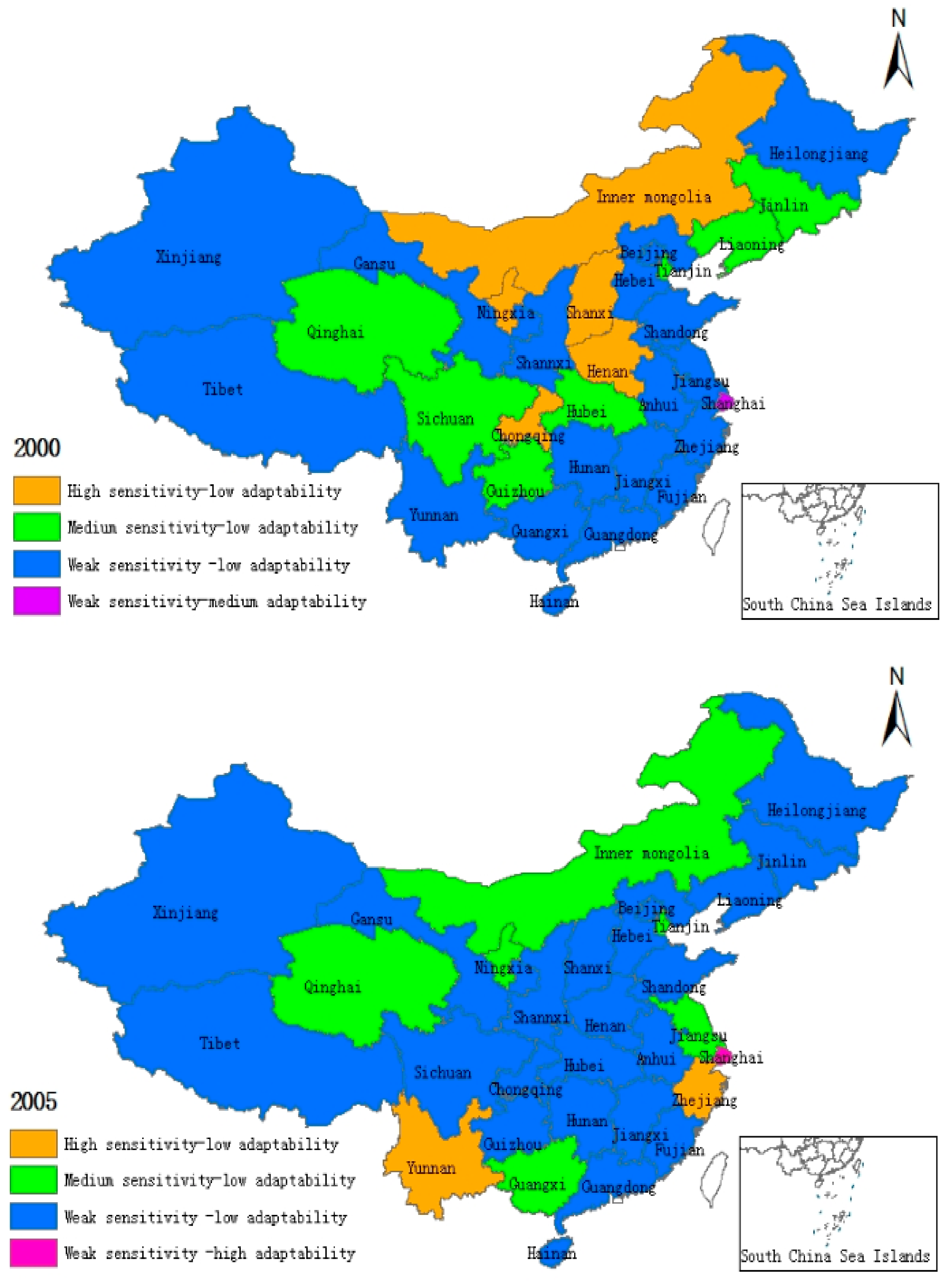
3.2. Vulnerability Types of Provincial Economies

Based on the changing spatial distribution of vulnerability types of provincial economies, economic vulnerability is characterized by the obvious spatial differentiation features, and economic vulnerability of the same type is in a state of aggregation (Figure 2). There are five types of economic vulnerability from 2000 to 2005, seven types in 2010, and eight types in 2014. Only the medium sensitivity–low adaptability type is absent. From 2000 to 2014, an apparent increase in economic vulnerability types and a diversified tendency can be seen. According to the change of economic vulnerability types, in 2000, most provinces in China belonged to the weak sensitivity–low adaptability type. Only five provinces belonged to the high sensitivity–low adaptability type: Chongqing, Henan, Shanxi, Inner Mongolia, and Ningxia. In 2014, nine provinces belonged to the high sensitivity–low adaptability type: Hainan, Guizhou, Guangxi, Xinjiang, Qinghai, Gansu, Inner Mongolia, Jilin, and Liaoning. High economic sensitivity and lack of higher economic adaptability lead to an increase in economic vulnerability, which will greatly affect the economic growth of these provinces. After 2010, there is a significant increase in the weak sensitivity–high adaptability type that only Jiangsu and Shanghai belonged to in 2010, but more provinces—that is, Guangdong, Shanghai, Beijing, Jiangsu, Anhui, Shandong, and Shaanxi—belonged to this type in 2014. The economic adaptability of some provinces has been observed to have improved, and, in the meantime, increased intervention and control imposed on economic sensitivity will lead to lower economic sensitivity. Overall, every province is characterized by the localization features of different economic sensitivity types during different time periods, which is a reflection of the complexity introduced by the economic vulnerability of a province.

4. Spatial Analysis of Economic Vulnerability

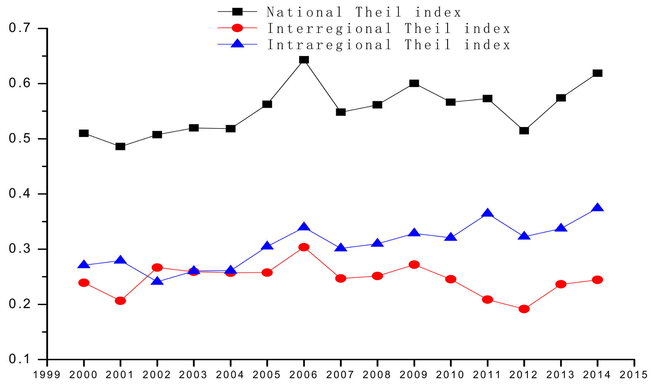
4.1. Analysis of Regional Differences of Economic Vulnerability

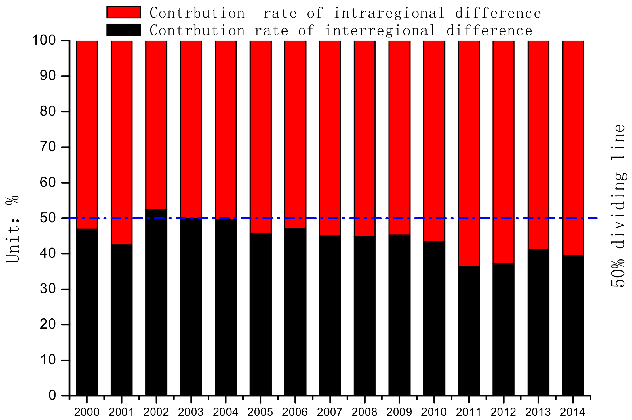
4.1.1. Interregional Difference in Economic Vulnerability

The regional difference in economic vulnerability shows an overall increasing trend, although regional differences vary in terms of range and tendency in different periods (Figure 3). From 2000 to 2006, the regional difference in economic vulnerability in China saw an obvious rising trend, especially from 2004 to 2006 when the rising range was significant, and the difference was maximum (0.6431) in 2006. The regional difference in economic vulnerability in China saw mild fluctuations from 2007 to 2012 and an obvious rising trend from 2012 to 2014.

The difference in intraregional economic vulnerability saw an obvious rising trend, while the interregional difference in economic vulnerability saw a slightly decreasing trend (Figure 4). After 2002, the difference in intraregional economic vulnerability gradually expanded, and in 2003 the difference value of intraregional economic vulnerability began to exceed the interregional difference value. After 2006, the interregional difference in economic vulnerability began to weaken significantly. From 2006 to 2014, the differences in economic vulnerability within and outside the region saw a significant rising trend.

After 2003, the contribution rates of the difference in intraregional economic vulnerability are constantly higher than those within the region. The difference values within the region are also constantly higher than those among regions, indicating that the difference in intraregional economic vulnerability is the primary cause for the generation of difference. Overall, the regional difference in economic vulnerability has gradually increased, especially from 2012 to 2014. The national Theil index has expanded and so has the intraregional difference, which is the main reason for the expansion of economic vulnerability difference.

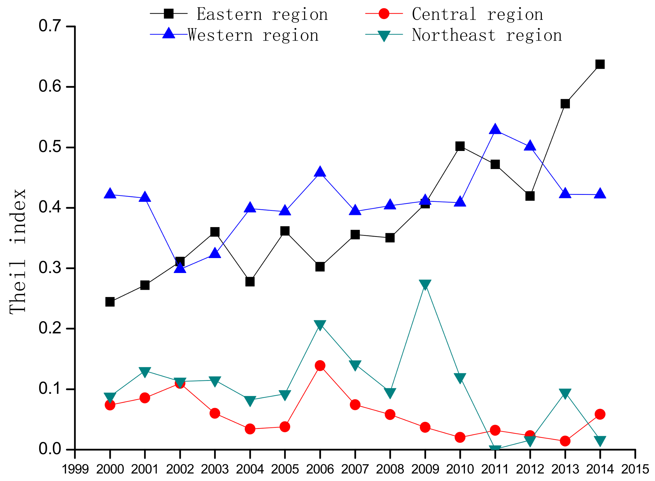
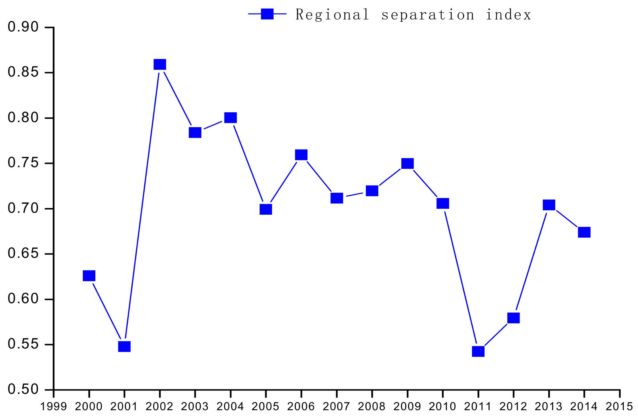
4.1.2. Characteristics of Regional Difference

According to the value and trend change of the Theil index of interregional differences in economic vulnerability of the four economic regions in China (Figure 5) from 2000 to 2014, the Theil indexes of the regional difference in economic vulnerability between the Eastern and Western regions are higher, and an overall trend of increasing differences through fluctuations can be seen. The Theil indexes of the regional difference in economic vulnerability between the Central and Northeast regions in China are lower, and an overall trend of decreasing differences through fluctuations can be seen. Different economic regions are characterized by different spatial structure features, even though there is some similarity between the Eastern and Western regions as well as between the Central and Northeast regions. Because different economic regions involve the economic growth of different provinces, the difference in economic vulnerability has shown regional characteristics of imbalance as follows: (1) In the Eastern region, from 2000 to 2003, a gradual expansion of difference can be seen; from 2004 to 2010, there is an overall trend of expanding difference through fluctuations; from 2011 to 2012, a slight decrease in the difference can be seen as well; from 2012 to 2014, the regional difference witnesses rapid expansion. Overall, the Theil index in the Eastern region is higher and the difference is larger. After 2012, the regional difference rapidly expanded, indicating that the spatial distribution pattern of 10 provinces in the eastern region is unbalanced and the provincial difference is huge; (2) In the Central region, from 2000 to 2005, a trend of steady decrease can be seen; the difference is maximum in 2006; after 2006, the regional difference gradually decreases. Taken as a whole, the Theil index in the central region is relatively smaller and the regional difference is little, indicating that economic vulnerability of the six provinces in this area is spatially characterized by a relative balance; (3) In the Western region, from 2000 to 2002, a trend of gradual decrease can be seen; from 2003 to 2006, there is a trend of gradual expansion; from 2007 to 2010, the difference is relatively stable; from 2011 to 2014, an obvious trend of decrease can be seen. Taken as whole, the Theil index in the Western region is relatively larger, which indicates that the regional difference is larger and characteristics of spatial distribution imbalance are prominent; after 2011, the regional imbalance shows a decreasing trend; (4) In the Northeastern region, from 2000 to 2005, a trend of steady decrease can be seen; the difference is maximum in 2006; in 2007 and 2008, the regional difference decreases; the difference value is maximum in 2009; in 2010 and 2011, it decreases to its minimum value; after 2011, the fluctuation is slight and the difference is little. Taken as whole, the Theil index in the Northeastern region is relatively smaller and the regional difference is little, which indicates that the economic vulnerability of the three provinces in this area is spatially characterized by a relative balance.

4.1.3. Complexity and Spatial Heterogeneity

Considering that economic regions are spatially separate from each other, the regional separation index will reflect the trend of the spatial structure evolvement of economic vulnerability differences. According to the formula of regional separation index, we take Tibet—whose economic aggregate is the lowest in China—as an example and calculate the regional separation index among the four economic regions in China from 2000 to 2014 (Figure 6). From 2001 to 2014, the regional separation index of economic vulnerability is characterized by a volatility curve; that is, a significant increase is followed by a gradual decrease, which indicates that economic vulnerability has gone through divergence and finally evolved towards convergence in terms of spatial structure in this period. In 2011, the regional separation index saw a significant change in inflection points, and the divergence of regional separation was strengthened, indicating that economic vulnerability has shown apparent complexity and spatial heterogeneity in terms of spatial structure.

4.2. Spatial Econometric Analysis of Eeconomic Growth and Economic Vulnerability

4.2.1. Taken as a Whole, Economic Growth and Economic Vulnerability Have a Negative Effect on Each Other, and Economic Vulnerability Has an Obvious Negative Spillover Effect on the Economic Growth of Neighbouring Provinces

The spatial econometric models, SLM, SEM, and SDM, all pass relevant tests and meet the requirements of the Akaike information criterion (AIC) and Schwarz information Criterion (SIC) for optimized model variables (AIC < SC). Based on the maximum log likelihood, the heightened SDM is an optimized model. The R-squared of the models are, respectively, 0.9926, 0.9910, and 0.9995, indicating that R-squared is higher, and the enactment of spatial econometric models basically meets the conditions for variable estimation.

The three models, SLM, SEM and SDM, show that production factors and technological levels have obvious positive effects on provincial economic growth, while economic vulnerability has obvious negative effects on provincial economic growth (

Table 5. Results of the spatial econometric models of economic growth and economic vulnerability.

Variable	Spatial Econometric Model
	SLM	SEM	SDM
$\ln A$	0.2498 *	0.2823 *	0.1071 ***
$\ln K$	0.5830 *	0.5593 *	0.5184 ***
$\ln L$	0.5395 *	0.5765 *	0.1323 ***
$V$	−0.2069 ***	−0.8171 ***	−0.0230 ***
$W\overline{\ln A}$	-	-	0.4907 *
$W\overline{\ln K}$	-	-	0.4590 *
$W\overline{\ln L}$	-	-	0.3266 *
$W\overline{V}$	-	-	-0.2605
$\rho W\ln Y$	0.065 **	-	0.032 ***
$\gamma W\epsilon$	-	0.1347 ***	0.590 ***
R-squared	0.9926	0.9910	0.9995
Sigma-square	0.0066	0.0081	0.0041
Log likelihood	33.7614	30.5272	75.3871
Akaike info criterion (AIC)	−55.5228	−51.0544	−138.774
Schwarz criterion (SC)	−46.9188	−43.8844	−130.17

Note: *, ** and *** respectively represent the significance levels of 1%, 5%, and 10%.

). SLM shows that the spatial lagged variable $\rho W\ln Y$ is 0.065 under a significance level of 5%, indicating that economic growth has a positive spillover effect on the economic growth of neighbouring provinces. SEM shows that the spatial disturbance variable $\gamma W\epsilon$ is 0.1347 under a significance level of 10%, indicating that production factors, technological levels, and economic vulnerability have obvious disturbing effects on economic growth. SDM shows that the spatial disturbance variable $\gamma W\epsilon$ is 0.590 under a significance level of 10%, indicating that the disturbing effect of production factors, technological levels, and economic vulnerability on economic growth has become stronger, and production factors and technological levels have a positive spillover effect on the economic growth of neighbouring provinces. The spatial interaction variable of economic vulnerability $W\overline{V}$ is −0.2605, which indicates that economic vulnerability has an obvious negative spillover effect on the economic growth of neighbouring provinces. Economic vulnerability not only hinders provincial economic growth but also greatly hinders the economic growth of neighbouring provinces.

4.2.2. Vulnerability and Spillover Effect on Neighbouring Provinces’ Economic Growth

Based on the spatial econometrics results of the Eastern, Central, Western, and Northeastern regions, the spatial econometric models, SLM, SEM, and SDM, all pass the relevant tests, and the R-squared is relatively high. The SLM, SEM, and SDM models of the Eastern, Central, and Northeastern regions all indicate that the economic vulnerability of these three regions has an obvious negative effect on economic growth, which in turn has a positive spillover effect on the economic growth of neighbouring provinces (

Table 6. Results of the spatial econometric models of economic growth and economic vulnerability in the Eastern, Central, Western, and Northeastern regions of China.

Variable	Eastern Region			Central Region			Western Region			Northeast Region
	SLM	SEM	SDM	SLM	SEM	SDM	SLM	SEM	SDM	SLM	SEM	SDM
$\ln A$	0.4527 *	0.4617 *	0.4509 ***	0.2310 *	0.2219 *	0.1737 ***	0.1345 *	0.1384 *	0.0934 ***	0.4402 *	0.4204 *	0.3924 ***
$\ln K$	0.7282 *	0.7138 *	0.7057 ***	0.5030 *	0.4929 *	0.4329 ***	0.2733 *	0.2844 *	0.2644 ***	0.6920 *	0.6242 *	0.6307 ***
$\ln L$	0.3723 *	0.4021 *	0.3976 ***	0.5798 *	0.5957 *	0.5639 ***	0.4927 *	0.5293 *	0.5264 ***	0.4024 *	0.4974 *	0.4229 ***
$V$	−0.1302 **	−0.5508 ***	−0.0103 ***	−0.3248 ***	−0.6242 ***	−0.1394 ***	−0.4023 ***	−0.8333 ***	−0.0923 ***	−0.1934 ***	−0.7134 ***	−0.1283 ***
$W\overline{\ln A}$	-	-	0.5739 *	-	-	0.5328 *	-	-	0.3293 *	-	-	0.4320 *
$W\overline{\ln K}$	-	-	0.6034 *	-	-	0.3843 *	-	-	0.0934 *	-	-	0.2193 *
$W\overline{\ln L}$	-	-	0.2684 *	-	-	0.3648 *	-	-	0.4284 *	-	-	0.2844 *
$W\overline{V}$	-	-	−0.1034	-	-	−0.2145	-	-	0.0528	-	-	−0.2605
$\rho W\ln Y$	0.1386 **	-	0.1023 ***	0.1118 **	-	0.0947 ***	0.0103 **	-	0.0072 ***	0.8013 **	-	0.0331 ***
$\gamma W\epsilon$	-	0.1384 ***	0.3720 ***	-	0.1634 ***	0.4632 ***	-	0.2743 **	0.7342 ***	-	0.1934 ***	0.4903 ***
R-squared	0.9304	0.9365	0.9936	0.9985	0.9962	0.9354	0.9926	0.9991	0.9923	0.9912	0.9945	0.9956
Sigma-square	0.0021	0.0074	0.0083	0.0073	0.0081	0.0053	0.0073	0.0078	0.0053	0.0067	0.0079	0.0056
Log likelihood	44.8465	40.8463	89.8343	39.3957	24.3947	103.9347	67.3552	70.3846	132.3745	56.2573	63.3856	118.322
Akaike info criterion (AIC)	−74.3956	−70.0544	−142.8446	−61.3957	−55.2947	−173.243	−89.3957	−101.3863	−193.3058	−80.993	−89.0375	−139.9304
Schwarz criterion (SC)	−70.9394	−68.4954	−138.3946	−56.3745	−54.3744	−167.234	−86.3856	−90.8353	−185.0358	−76.3346	−83.8574	−133.8322

Note: *, ** and *** respectively represent the significance levels of 1%, 5%, and 10%.

). Economic vulnerability has an obvious disturbing effect on economic growth, and it also has an obvious negative spillover effect on the economic growth of neighbouring provinces. Thus, within these three regions, economic vulnerability not only hinders provincial economic growth, but also greatly hinders the economic growth of neighbouring provinces. The SLM and SEM of the Western region show that economic vulnerability has an obvious negative effect on economic growth, which in turn has a positive spillover effect on the economic growth of neighbouring provinces. The SDM model of the Western region shows that the spatial interaction variable of economic vulnerability $W\overline{V}$ is 0.052, indicating that economic vulnerability has a slight positive spillover effect on the economic growth of neighbouring provinces. Therefore, while the economic vulnerability of provinces in the Western region has a disturbing effect on provincial economic growth, it somehow facilitates the economic growth of neighbouring provinces. The reason is that the economic vulnerability of some provinces in the Western region is higher, and the strength of their economic growth is weaker than that of other places; moreover, to realize economic growth targets, the Chinese government provides financial and policy support, which benefits neighbouring provinces in similar situations and promotes their economic growth as well.

5. Conclusions and Discussion

5.1. Conclusions

There are great differences in the economic vulnerability among provinces. The economic vulnerability of the Western provinces of China is higher, and the fluctuation range is large. The provincial economic vulnerability is characterized by obvious spatial difference, and economic vulnerability of the same type is spatially aggregated. The types of economic vulnerability have significantly increased, and their characteristics of localization are evident. Thus, a complicated state of economic vulnerability can be seen.

Interregional economic vulnerability has gradually increased, and intraregional difference is the main cause of economic vulnerability differences. The difference in economic vulnerability between Eastern and Western China is higher, showing spatial pattern characteristics of prominent and reinforcing regional imbalance. The difference in economic vulnerability between Central and Northeast China is lower, showing spatial pattern characteristics of declining regional imbalance. The trend of spatial structure evolution of economic vulnerability is characterized by a volatility curve. Regional separation and divergence have been strengthened, and complexity and spatial heterogeneity can be seen in terms of spatial structure.

The growth of China’s provincial economies and economic vulnerability are negatively related. In Eastern, Central, and Northeast China, the vulnerability of provincial economies has an obvious negative spillover effect on the economic growth of neighbouring provinces. In Western China, the vulnerability of provincial economies has a slight positive spillover effect on the economic growth of neighbouring provinces.

5.2. Discussion

The vulnerability of China’s provincial economies is essentially a consequence of the combined effects of sensitivity and adaptability in economic subsystems, social subsystems, and nature–resource–environmental subsystems. Economic growth at a provincial spatial scale is characterized by different localization features in terms of economic growth factors, such as population, geographic location, environment, resource endowment, economic development level, and economic stage; thus, economic vulnerability at different regional spatial scales show different representations and there is significant regional difference in spatial distribution. It is an urgent need for us to adopt regulatory measures according to localization features of the vulnerability of China’s provincial economies to further promote sustainable growth of China’s provincial economies.

With regard to the vulnerability of China’s provincial economies, a clear sense of regulation direction and regulation measures of economic vulnerability will contribute to the reduction of economic vulnerability. The main measures taken to reduce the vulnerability of China’s provincial economies include the establishment of an industry security prewarning system, the establishment and implemention of a scientific industrial security development plan, and finance-based supply-side structural reforms aiming to serve the real economy and strengthen financial regulation. Furthermore, we should also intensify our efforts to fight poverty and redouble our efforts to build a healthy China. We should adopt diversified methods of environmental governance, increase investment in environmental governance, and strengthen the construction of an environmental legal system. We should change the mode of urbanization development, promote city agglomeration construction with a focus on the construction of characteristic towns, and put economic vulnerability in the context of the implementation of urban planning and construction to build a new type of urbanization. We should aim to set up a good institutional environment for scientific and technological innovations, and implement a system construction that promotes development through innovation to make China an innovative nation. We should also aim to form the factor -price -oriented market mechanism, encourage supply-side structural reforms, and allocate resources according to market prices. In addition, economic vulnerability should be seen in the context of regional economic planning.

Current studies of regional economic growth have been mostly carried out in terms of the theory, model, and structure of economic growth from a positive perspective, and there are few economic vulnerability studies that examine the potential negative effects on sustainable economic growth. Using the VSD model, this study adopts the multilevel extension assessment method to conduct a comprehensive assessment of provincial economic vulnerability in China. Although previous research on the essential attributes of economic vulnerability is adequate, economic vulnerability theory needs further attention.

Economic vulnerability assessment is an important part of economic vulnerability studies. There are many quantitative assessment methods, and abundant research results have been achieved. Due to the complexity of the economic system and different perspectives for interpreting the concept of economic vulnerability, there is some controversy about the assessment model, assessment index, and assessment result of economic vulnerability. Therefore, this study uses a multilevel extension assessment method to conduct a comprehensive assessment of provincial economic vulnerability in China, and scientific conclusions have been drawn. However, comprehensive assessments from the perspective of economic growth are few, thus there is lack of result comparisons using different assessment methods. In further research, we will compare this with other assessment methods to optimize and adjust the multilevel extension assessment method, while a contrasting quantitative with qualitative case-study research will be included.

Nevertheless, the multilevel extension assessment method has its limitations. In the assessment process, the setting of grade theory domains has a certain degree of subjectivity. Index selection of an assessment factor set should be more scientific, and classical domains and joint domains should be determined by strict standards. Moreover, this assessment method only focuses on the degree and trend of economic vulnerability, and does not pay enough attention to the early warning assessment of economic vulnerability in the future.

This article analyses the interactive relation between economic growth and economic vulnerability from a spatial perspective. In the future, study of the spatial generation mechanism, influence factor, and spatial evolution process will help clarify the spatiotemporal pattern change of economic vulnerability and determine vulnerability factors in economic growth so that we can exert effective regulation and forewarning, and reduce economic vulnerability to achieve economic growth sustainability.

References

1. Birkmannn, J. Measuring Vulnerability to Natural Hazards: Towards Disaster Resilient Societies; United Nations University Press: Tokyo, Japan, 2006. [Google Scholar]
2. Fang, C.; Wang, Y. A comprehensive assessment of urban vulnerability and its spatial differentiation in China. Acta Geogr. Sin. 2015, 70, 234–247. (In Chinese) [Google Scholar] [CrossRef]
3. Kates, R.W.; Clark, W.C.; Corell, R.; Hall, J.M.; Jaeger, C.C.; Lowe, I.; McCarthy, J.J.; Schellnhuber, H.J.; Bolin, B.; Dickson, N.M.; et al. Environment and development: Sustainability science. Science 2001, 292, 641–642. [Google Scholar] [CrossRef] [PubMed]
4. Shi, P.; Wang, J.; Chen, J.; Ye, T.; Zhou, H. The future of human-environment interaction research in geography: lessons from the 6th open Meeting of IHDP. Acta Geogr. Sin. 2006, 61, 115–126. (In Chinese) [Google Scholar]
5. Li, H.; Zhang, P.; Chen, Y. Concepts and assessment methods of vulnerability. Progr. Geogr. 2008, 27, 18–25. (In Chinese) [Google Scholar]
6. Cutter, S.L. The vulnerability of science and the science of vulnerability. Ann. Assoc. Am. Geogr. 2003, 93, 1–12. [Google Scholar] [CrossRef]
7. Cutter, S.L. Vulnerability to environmental hazards. Progr. Hum. Geogr. 1996, 20, 529–539. [Google Scholar] [CrossRef]
8. Birkmann, J.; Cardona, O.D.; Carreño, M.L.; Barbat, A.H.; Pelling, M.; Schneiderbauer, S.; Kienberger, S.; Keiler, M.; Alexander, D.; Zeil, P.; et al. Framing vulnerability, risk and societal responses: The MOVE framework. Nat. Hazards 2013, 67, 193–211. [Google Scholar] [CrossRef]
9. Briguglio, L. Preliminary Study on the Construction of an Index for Ranking Countries According to their Economic Vulnerability; UNCTAD: Geneva, Switzerland, 1992. [Google Scholar]
10. Saldaña-Zorrilla, S.O. Reducing Economic Vulnerability in Mexico. Natural Disasters, Foreign Trade and Agriculture. Ph.D. Thesis, WU Vienna University of Economics and Business, Vienna, Austria, 2006. [Google Scholar]
11. Guillaumont, P. On the Economic Vulnerability of Low Income Countries; Mimeo, CERDI-CNRS, Université d’Auvergne: Auvergne, France, 1999. [Google Scholar]
12. Briguglio, L.G.; Farrugia Cordina, N.; Vella, S. Economic vulnerability and resilience: Concepts and measurements. Oxf. Dev. Stud. 2009, 37, 229–247. [Google Scholar] [CrossRef]
13. Kienberger, S.; Hagenlocher, M. Spatial-explicit modeling of social vulnerability to malaria in East Africa. Int. J. Health Geogr. 2014, 13, 29. [Google Scholar] [CrossRef] [PubMed]
14. Briguglio, L.; Kisanga, E.J. Economic Vulnerability and Resilience of Small S Vulnerability and Spillover Effect on Neighbouring Provinces’ Economic Growth States; Islands and Small States Institute of the University of Malta and Commonwealth Secretariat: Msida, Malta, 2004. [Google Scholar]
15. Hallegatte, S. Economic Resilience: Definition and Measurement. Soc. Sci. Electron. Publ. 2014, a2, 291–299. [Google Scholar]
16. Rose, A.; Krausmann, E. An economic framework for the development of a resilience index for business recovery. Int. J. Disaster Risk Reduct. 2013, 5, 73–83. [Google Scholar] [CrossRef]
17. Gong, H.; Hassink, R. Regional Resilience: The Critique Revisited. In Creating Resilient Economies: Entrepreneurship, Growth and Development in Uncertain Times; Williams, N., Vorley, T., Eds.; Edward Elgar: Cheltenham, UK, 2017; pp. 206–216. [Google Scholar]
18. Hu, X.; Hassink, R. Exploring adaptation and adaptability in uneven economic resilience: A tale of two Chinese mining regions. Camb. J. Reg. Econ. Soc. 2017, 10, 527–541. [Google Scholar] [CrossRef]
19. Martin, R.; Sunley, P. On the notion of regional economic resilience: Conceptualization and explanation. J. Econ. Geogr. 2015, 15, 1–42. [Google Scholar] [CrossRef]
20. Su, F.; Zhang, P.Y. Vulnerability assessment of petroleum city’s economic system based on set pair analysis: A case study of Daqing city. Acta Geogr. Sin. 2010, 65, 454–464. (In Chinese) [Google Scholar]
21. Yang, A.; Wu, J. The relationship between Chinese economic system vulnerability and sustainable development: 15 years sample. Reform 2012, 2, 25–33. (In Chinese) [Google Scholar]
22. Sun, P.; Xiu, C. Study on the vulnerability of economic development in mining cities based on the PSE Model. Geogr. Res. 2011, 30, 301–309. (In Chinese) [Google Scholar]
23. Feng, Z. Study of Vulnerability and Optimization Control of Economic Development in West China; Tianjin University: Tianjin, China, 2003. (In Chinese) [Google Scholar]
24. Zhao, G.; Zhang, W. A study on vulnerability of the region economies and society: Hebei. Shanghai Econ. Res. 2006, 1, 65–69, 96. (In Chinese) [Google Scholar]
25. Ren, C.; Zhai, G.; Li, S.; Wu, Y. Regional differences of Chinese economic growth system vulnerabilities from the perspective institutional factors. Chin. J. Agric. Resour. Reg. Plan. 2017, 38, 10–19. (In Chinese) [Google Scholar]
26. Wang, Y.; Fang, C. Urban vulnerability: Progress and prospect. Progr. Geogr. 2013, 32, 755–768. (In Chinese) [Google Scholar]
27. Min, T. China’s Economy: Alert to Black Swans; Publishing House of Electronics Industry: Beijing, China, 2013. (In Chinese) [Google Scholar]
28. Li, L.; Zhang, M. The institutional reform and development transformation of economic growth rate change period—The eighth China economic growth and cycle BBS review. Econ. Res. J. 2014, 10, 79–183. (In Chinese) [Google Scholar]
29. Bootle, R. How Much is the Financial Sector Contributing to the Real Economy? Take 15 Series; Webcasts & Podcasts: London, UK, 2016. [Google Scholar]
30. He, L.; Zhang, P.Y. The evolution and coping timing of economic vulnerability of mining cities: A case study in northeast China. Econ. Geogr. 2014, 34, 82–88. (In Chinese) [Google Scholar]
31. He, L.; Zhang, P.Y. Economic system vulnerability of mining cities in Northeast China. J. China Coal Soc. 2008, 33, 116–120. (In Chinese) [Google Scholar]
32. He, L.; Zhang, P.Y. Vulnerability of urban employment of mining cities in northeast China. Geogr. Res. 2009, 28, 751–760. (In Chinese) [Google Scholar]
33. Zhao, X.; Xiao, F. Evaluation research about the Marine disaster vulnerability of coastal areas-in the case of the typhoon disasters in Shandong province. Mar. Econ. 2013, 3, 21–25. (In Chinese) [Google Scholar]
34. Li, B.; Han, Z. Regional system vulnerability of man-land relationship in coastal cities—A case Dalin city. Econ. Geogr. 2010, 30, 1722–1728. (In Chinese) [Google Scholar]
35. Li, B.; Han, Z. Application of Markov Chain Model in study on periodicity of climate change in Daihai region. Geogr. Geo-Inf. Sci. 2010, 26, 78–81, 86. (In Chinese) [Google Scholar]
36. Li, B.; Yang, Z.; Su, F. Measurement of vulnerability in human-sea economic system based on set pair analysis: A case study of Dalian city. Geogr. Res. 2015, 34, 967–976. (In Chinese) [Google Scholar]
37. Li, F. Study of vulnerability measurement of Chinese tourism economic: Based on SPA. Tour. Sci. 2013, 27, 15–28. (In Chinese) [Google Scholar]
38. Liang, Z.; Xie, L. On the vulnerability of economic system of traditional tourism cities—A case from Guilin. Tour. Tribe 2011, 26, 40–46. (In Chinese) [Google Scholar]
39. Liu, Y.; An, L.; Jin, T. Quality of economic growth of China under the background of imbalanced economic structure. J. Quant. Tech. Econ. 2014, 2, 20–35. (In Chinese) [Google Scholar]
40. Wang, X. The fundamental reason for the slowdown in economic growth is the structural imbalances. Henan Soc. Sci. 2015, 4, 23–35. (In Chinese) [Google Scholar]
41. Adger, W.N. Vulnerability. Glob. Environ. Chang. 2006, 16, 268–281. [Google Scholar] [CrossRef]
42. Fang, X.; Yuan, P. Review on the Three Key Concepts of Resilience, Vulnerability and Adaptation in the Research of Global Environmental Change. Prog. Geogr. 2007, 26, 11–22. (In Chinese) [Google Scholar]
43. Gao, C.; Jin, F.; Li, J. Vulnerability assessment of economic system of Oasis cities in arid area. Econ. Geogr. 2012, 32, 43–49. (In Chinese) [Google Scholar]
44. Gallopin, G.C. A Systemic Synthesis of the Relations between Vulnerability, Hazard, Exposure and Impact, Aimed at Policy Identification. In Economic Commission for Latin American and the Caribbean (ECLAC) Handbook for Estimating the Socio-Economic and Environmental Effects of Disasters; ECLAC: Mexico City, Mexico, 2003; pp. 2–5. [Google Scholar]
45. Gallopin, G.C. Linkages between vulnerability, resilience, and adaptive capacity. Glob. Environ. Chang. 2006, 16, 293–303. [Google Scholar] [CrossRef]
46. Polsky, C.; Neff, R.; Yarnal, B. Building comparable global change vulnerability assessments: The vulnerability scoping diagram. Glob. Environ. Chang. 2007, 17, 472–485. [Google Scholar] [CrossRef]
47. Luers, A.L.; Lobell, D.B.; Sklar, L.S.; Addams, L.C.; Matson, P.A. A method for quantifying vulnerability, applied to the agricultural system of the Yaqui V alley, Mexico. Glob. Environ. Chang. 2003, 13, 255–267. [Google Scholar] [CrossRef]
48. Luers, A.L. The surface of vulnerability: An analytical framework for examining environmental change. Glob. Environ. Chang. 2005, 15, 214–223. [Google Scholar] [CrossRef]
49. Acosta-Michlik, L.; Mark, R. From Generic Indices to Adaptive Agents: Shift Foci in Assessing Vulnerability to the Combined Impacts of Climate Change and Globalization. IHDP Newsl. 2005, 1, 14–16. [Google Scholar]
50. Adger, W.N.; Brooks, N.; Bentham, G.; Eriksen, S.H. New Indicators of Vulnerability and Adaptive Capacity; Technical Report No.7; Tyndall Centre for Climate Change Research: Norwich, UK, 2004. [Google Scholar]
51. Smit, B.; Burton, I.; Klein, R.J.T.; Wandel, J. An Anatomy of Adaptation to Climate Change and Variability. Clim. Chang. 2000, 45, 223–251. [Google Scholar] [CrossRef]
52. Smit, B.J.; Wandel, J. Adaptation, adaptive capacity and vulnerability. Glob. Environ. Chang. 2006, 16, 282–292. [Google Scholar] [CrossRef]
53. Briguglio, L. Small island states and their economic vulnerabilities. World Dev. 1995, 23, 1615–1632. [Google Scholar] [CrossRef]
54. Crowards, T. An Economic Vulnerability Index for Developing Countries with Special Reference to Caribbean (Alternative Methodologies and Provisional Results): A Summary of the Draft for Consultation; Caribbean Development Bank: St. Michael, Barbados, 1999. [Google Scholar]
55. Wang, C. Reconsidering the economic vulnerability index of the United Nations. Can. J. Dev. Stud. 2013, 34, 553–568. [Google Scholar] [CrossRef]
56. He, Y.; Huang, X.; Zhai, L. Assessment and influencing factors of social vulnerability to rapid urbanization in urban fringe: A case study of Xi’an. Acta Geogr. Sin. 2016, 71, 1315–1328. (In Chinese) [Google Scholar]
57. Yuan, H.; Niu, F.; Gao, X. Establishment and application of an urban economic vulnerability evaluation system. Acta Geogr. Sin. 2015, 70, 271–282. (In Chinese) [Google Scholar]
58. Shannon, C.E.; Weaver, W. The Mathematical Theory of Communication; The University of Illinois Press: Champaign, IL, USA; Urbana: St. Louis, MI, USA, 1947. [Google Scholar]
59. Rubinstein, R.Y.; Kroese, D.P. The Cross-Entropy Method; Springer: New York, NY, USA, 2004. [Google Scholar]
60. Wen, C. Matter-Element Model and Its Application; Scientific and Technological Literature Publishing House: Beijing, China, 1994. (In Chinese) [Google Scholar]
61. Cai, W.; Yang, C.; Wang, G. A new interdisciplinary subject—Extenics. Bull. Natl. Nat. Sci. Found Chin. 2004, 18, 268–272. (In Chinese) [Google Scholar]
62. Cai, W.; Yang, C. The basic theory and method system of Extenics. Chin. Sci. Bull. 2013, 58, 1190–1199. (In Chinese) [Google Scholar] [CrossRef]
63. Zheng, G.; Jing, Y.; Huang, H.; Zhang, X.; Gao, Y. Application of life cycle assessment (LCA) and extenics theory for building energy conservation assessment. Energy 2009, 34, 1870–1879. [Google Scholar] [CrossRef]
64. Wang, M.; Xu, X.; Li, J.; Jin, J.; Shen, F. A novel model of set pair analysis coupled with extenics for evaluation of surrounding rock stability. Math. Probl. Eng. 2015, 2015, 1–9. [Google Scholar] [CrossRef]
65. Theil, H. Economics and Information Theory; North-Holland Publishing Company: Amsterdam, The Netherlands, 1967. [Google Scholar]
66. O’Kelly, G.S.; Pakes, A. The Dynamics of Productivity in the Telecommunications Equipment Industry. NBER Work. Pap. 1992, 64, 1263–1297. [Google Scholar]
67. Ming, L.; Zhao, C. Fragmented growth: Why economic opening may worsen domestic market segmentation? Econ. Res. J. 2009, 3, 42–52. (In Chinese) [Google Scholar]
68. Yao, L.; Gu, G. The evolution of ecology and environmental response to the regional economic integration and the influence factors in Jilin province. Sci. Geogr. Sin. 2014, 34, 464–471. (In Chinese) [Google Scholar]
69. Hu, X. The Spatial Neighbor Effect of Institutional Change; Shanghai Academy of Social Sciences: Shanghai, China, 2016. (In Chinese) [Google Scholar]
70. Anselin, L.; Bera, A. Spatial dependence in linear regression models with an introduction to spatial Econometrics. In Handbook of Applied Economic Statistics; Marcel Dekker: New York, NY, USA, 1998; pp. 19–44. [Google Scholar]
71. Lesage, J.P.; Pace, R.K. Interpreting Spatial Econometric Models; Springer: Berlin, Germany, 2014. [Google Scholar]
Figure 1. Fluctuation map of the economic vulnerability of several provinces in China from 2000 to 2014.
Sustainability 10 01261 g001
Figure 2. Spatial distribution map of economic vulnerability types of China’s provinces (2000, 2005, 2010, and 2014).
Sustainability 10 01261 g002aSustainability 10 01261 g002b
Figure 3. Trend change of the Theil Index of economic vulnerability from 2000 to 2014.
Sustainability 10 01261 g003
Figure 4. Contribution rates of intraregional and interregional differences of economic vulnerability from 2000 to 2014.
Sustainability 10 01261 g004
Figure 5. Trend of the Theil Index of the regional difference in economic vulnerability between the four regions from 2000 to 2014.
Sustainability 10 01261 g005
Figure 6. Trend of regional separation index of economic vulnerability from 2000 to 2014.
Sustainability 10 01261 g006