Abstract
This paper focuses on alternatives to the CAFC-NEV credits policy in the automotive industry of China. It considers a dual-channel supply chain consisting of a manufacturer and a retailer that can simultaneously produce and sell new energy vehicles (NEVs) and internal combustion engine vehicles (ICEVs). Differential game theory is employed to explore dynamic optimal decisions under CAFC-NEV credits and carbon credit policies. The results suggest that the strategies combining CAFC-NEV credits and carbon credit policies are equivalent to a single CAFC-NEV credits policy. Therefore, implementing the carbon credit policy on the basis of the CAFC-NEV credits policy does not affect the increase in NEV range. If the NEV credit score is below a certain threshold, the carbon credit policy will result in a higher range increase and brand goodwill of NEV. In the transition process of implementing the carbon credit policy based on CAFC-NEV credits and subsequently canceling the CAFC-NEV credit policy, the profits of supply chain members change slightly. The findings provide a theoretical basis for the timely exit of the CAFC-NEV credits policy.
1. Introduction
The transportation industry is an important sector of energy consumption and carbon dioxide emissions. The carbon emission in China from the transportation sector accounts for about 10% to 12% of the national total, making it the third-largest emission source after electricity and industry (Wu et al., 2025) [1]. To reduce carbon emissions from the transportation sector and strive to reach the carbon peak as soon as possible, China is actively promoting low-carbon transportation methods and accelerating the NEV popularization. The production and sales of NEVs have exceeded 12 million in 2024 and 16 million in 2025, making it the first country in the world to reach 10 million, and the market penetration rate of NEVs reached 50.8%, achieving the 2035 Nationally Determined Contributions, that is, NEVs are the main type of new vehicle sales. With the vigorous development of the NEV industry and the introduction of carbon emission control measures, the adjustment of CAFC-NEV credits in the automotive industry is necessary, and alternatives are available.
Therefore, this paper focuses on three aspects of the automotive supply chain: the decision of the automotive supply chain, dual-channel, and alternatives to the CAFC-NEV credits policy. It introduces a review of relevant literature in these three research areas.
- (1)
- Decisions of automotive supply chain members
The decisions of automotive supply chain members include emissions reduction, R&D, price strategy, quality strategy, marketing strategy, services, and other aspects (Zhou et al., 2023; Yi et al., 2024; Xing and Wang, 2025; Adnan et al., 2025) [2,3,4,5], among which price strategy is the main focus of scholars. For example, Gong et al. (2022) [6] established the game model of centralized and decentralized decisions in the NEV supply chain to study the impact of consumers’ low-carbon preferences on supply chain price and member profits. Zhao et al. (2022) [7] constructed a supply chain model of NEVs and ICEVs composed of automaker and retailer, compared the price, demand, and supply chain profits under different decision models, and designed a joint mechanism of revenue sharing and ex-factory price negotiation contract. Overall, research on price strategy for the automotive supply chain is relatively mature.
- (2)
- Dual-channel supply chain
The dual-channel supply chain has received widespread attention from academia because studies on the single-channel supply chain neglected the direct sales channel. A manufacturer may sell products through both retail and direct sales channels (Ji et al., 2017) [8]. Chiang et al. (2003) [9] argued that manufacturers could stimulate demand in the retail channel by prompting retailers to lower prices after introducing a direct sales channel. Zhou and Ye (2018) [10] introduced joint emission reduction into a dual-channel supply chain framework to address the environmental and economic benefits of recycling retired batteries from NEVs. Recent studies explore some emerging forms of direct sales. For example, Liu et al. (2021) [11] constructed a dual-channel supply chain in which manufacturers sell new products through retail channels and their own online channel, which shows that manufacturers’ production and optimal price strategies depend on production cost and channel sales cost. Yu et al. (2025) [12] examined whether a manufacturer decides to introduce a livestream channel based on a traditional resale channel. The results reveal that the competitor does not adopt livestream, and the manufacturer’s choice to adopt livestream depends on product substitutability. Our study expands upon the above research by constructing a dual-channel supply chain model for NEVs and ICEVs, consisting of automaker and retailer, and comparing the impact of key policy parameters on equilibrium solutions under decentralized and centralized decisions.
- (3)
- Carbon emission management policies to replace CAFC-NEV credits
The Ministry of Industry and Information Technology has proposed transforming existing CAFC-NEV credits into a carbon emission management policy. Related research has paid considerable attention to this issue, with some scholars examining automobile carbon tax, carbon allowance, and carbon credit, and demonstrating the effectiveness of these emission reduction pathways. The carbon tax is a fiscal measure that taxes carbon emissions from automobiles. China has not yet established a corresponding carbon tax system for carbon emission, mainly because it is difficult to set a reasonable tax rate and there are controversies (Ning et al., 2024; Du et al., 2024) [13,14]. Therefore, the possibility of imposing a carbon tax on automobiles is relatively low. Compared to the carbon tax, carbon allowance and carbon credit are market-based measures. Carbon allowance refers to the emission allowance allocated by the government to key emitting entities for a specified period (Shojaei and Mokhtar, 2022) [15]. Some scholars examined the promotion strategies of NEV from a static perspective using game theory models and system dynamics models under carbon allowance constraints (Yin and Liu, 2021; Wang et al., 2025; Wang et al., 2025) [16,17,18]. Other studies explored the optimal production decision of NEVs under CAFC-NEV credits and carbon allowance from a dynamic perspective (He et al., 2023) [19]. However, CAFC-NEV credits and carbon allowance are both market-based instruments, and it is almost impossible for them to appear in the production process at the same time in reality. Existing research on carbon credit is relatively limited, with Sun (2021) being the first to propose this concept [20]. Liu and Kong (2024) pointed out that carbon credit is an effective policy tool that compensates for the shortcomings of CAFC-NEV credits, which are only applied to the production stage by providing low-carbon travel incentives at the usage stage [21].
The central topic of the above literature is the production decision of ordinary supply chains without policy constraints. Therefore, this paper establishes a differential game model for a supply chain capable of simultaneously producing and selling both NEV and ICEV to analyze the impact of CAFC-NEV credits and carbon credit policies on the demand for these two types of vehicles. Compared to previous research, it may offer the following marginal contributions:
- (1)
- This paper is one of the few quantitative studies that explores carbon credit for NEV, and it is one of the earliest studies to analyze the optimal decision-making of the automotive supply chain from a dynamic perspective under the constraint of carbon credit policy.
- (2)
- Considering the retail channel of the retailer and the direct sales channel of the manufacturer, CAFC-NEV credits and carbon credits are incorporated into the dual-channel supply chain framework to examine the optimal strategies of the manufacturer and retailer in the dual-channel supply chain.
- (3)
- The potential impact of the cancellation for the CAFC-NEV credits is explored through model derivation and numerical examples. The incentive effect of the carbon credit on the development of NEVs is evaluated, which provides a reference for the withdrawal of the CAFC-NEV credits policy.
2. Hypothesis of the Study and Basic Model
Assumption 1.
Range anxiety and battery performance degradation are significant factors restricting the widespread adoption of NEV (Wu et al., 2024; Hu et al., 2024) [22,23]. Automakers are investing in innovative technologies such as Cell to Pack (CTP) and Cell to Chassis (CTC) to achieve large-scale applications, which significantly improve the energy density of battery packs, further reducing consumers’ range anxiety. In addition, battery degradation cannot be ignored. As the number of charge–discharge cycles increases, the battery capacity gradually decreases, leading to a reduction in driving range. Therefore, we construct the following difference model to describe the dynamics of NEV range increase.
where R(t) represents the NEV range increase at time t, we assume that the initial range R(0) = 0, I(t) is the manufacturer’s endurance effort, η > 0 denotes the range sensitivity of the endurance effort, and δR > 0 indicates the endurance depreciation.
Assumption 2.
Goodwill is formed from brand awareness, and marketing activities contribute to consumers’ clearer awareness, thereby promoting the improvement in brand goodwill. Brand goodwill is memory-dependent; market competition, consumer forgetting, and negative events can lead to the natural depreciation of goodwill (Li, 2026) [24]. Moreover, manufacturers’ endurance effort can improve product performance and promote goodwill accumulation (Hemmelder et al., 2025; Lin and Zhang, 2026) [25,26]. We thus assume that the brand goodwill of NEVs is positively impacted by the NEV range increase. By introducing the impact of NEV range increase on goodwill, we modify the Nerlove-Arrow model as follows.
where G(t) represents NEV brand goodwill, and the initial goodwill is assumed to be G(0) = 0. A(t) represents the marketing effort of the retailer, with φ > 0 and θ > 0 representing the goodwill sensitivity of endurance and marketing efforts, respectively, and η > 0 reflecting the goodwill depreciation.
Our model differs from the Nerlove-Arrow model in that the NEV range increase is one of the factors in establishing the NEV brand goodwill and positively affects it.
Assumption 3.
Zhang et al. (2016) and Yi et al. (2022) [27,28] argue that market demand is a linear expression of price and non-price factors. This paper assumes that the NEV market demand is influenced by price, NEV range increase, and brand goodwill. Based on observations of reality, range anxiety is a major concern for NEV users or potential users (Wang et al., 2023; Huang et al., 2024) [29,30]. Range improvement contributes to enhancing confidence among consumers and promoting NEV consumption. Some scholars, such as Li (2026) [24], Yi et al. (2024) [3], and Long et al. (2022) [31], also pay attention to consumers’ brand preference, and goodwill positively influences consumers’ purchasing decisions for NEVs. Meanwhile, considering the competition between NEVs and ICEVs, the improvement in NEV range and the accumulation of brand goodwill will reduce the consumer demand for ICEVs.
In a single-channel supply chain, the manufacturer sells products solely through the retail channel, and the market demand functions for NEV and ICEV are characterized as follows.
where M represents the market capacity, k represents the market share of NEVs, β1 and β2 represent the price sensitivity of NEVs and ICEVs, respectively, and χ1, χ2, and ϕ1, ϕ2 represent the marginal impact of NEVs’ brand goodwill and range increase on the demand for the two types of vehicles, respectively.
In a dual-channel supply chain, the manufacturer sells products through both retail and direct sales channels. The demand functions for NEV and ICEV through retail and direct sales channels are expressed as follows.
where the subscripts i and d represent retail and direct sales channels, respectively, 0 ≤ μ1 ≤ 1 and 0 ≤ μ2 ≤ 1 represent consumer loyalty to the retail channel, p1i and p2i represent the prices of NEVs and ICEVs in the retail channel, p1d and p2d represent the prices in the direct sales channel, and ξ1 and ξ2 represent cross-price sensitivity.
For ease of comparison with a single channel, following Yi et al. (2024) [3], we define β1i − ξ1 + β1d − ξ1 = β1, β2i − ξ2 + β2d − ξ2 = β2. The above demand function can be rewritten as follows.
According to relevant research (Li et al., 2016; Zhou and Ye, 2018; Yi et al., 2022) [10,28,32], in order to reduce channel conflict, it is assumed that a unified price strategy is adopted, i.e., p1i = p1d, p2i = p2d. Therefore, the final demand functions are as follows.
where θ1 = (β1i − ξ1)/β1, (1 − θ1) = (β1d − ξ1)/β1, θ2 = (β2i − ξ2)/β2, (1 − θ2) = (β2d − ξ2)/β2, representing the relative proportions of price sensitivity of NEVs and ICEVs in retail channel and direct sales channel, respectively, 0 < θ1 <1, 0 < θ2 <1.
Assumption 4.
Based on relevant research (Lambertini, 2018; Kazancoglu et al., 2022; Sun et al., 2025) [33,34,35], we assume that the range and marketing cost functions are quadratic functions of range effort and marketing effort, respectively, in the following form.
where km > 0, kr > 0, represent the cost coefficients of the corresponding variables.
Assumption 5.
CAFC-NEV credits consist of two parts: corporate average fuel consumption (CAFC) credit and new energy vehicle (NEV) credit. CAFC credit requires automakers to ensure that the average fuel consumption of passenger vehicles meets national standards. Failure to meet these standards results in negative credit, which companies must purchase to make up for. Meanwhile, to encourage automakers to produce NEVs, companies can earn positive credits (NEV), which can be used to offset negative CAFC credits or sold to other manufacturers. The calculation formulas are as follows.
where b is the CAFC compliance value, a is the actual CAFC value, α1 is the NEV credit score, and α2 is the required proportion of NEV credit.
Assumption 6.
A carbon credit is an emission reduction reward that encourages users to use NEVs. It quantifies the contribution of NEV travel to carbon emission reduction compared to ICEV, and registers it as a carbon credit. NEV owners can benefit by trading carbon credits (Liu and Kong, 2024) [21].
Carbon credit essentially reduces the net price and total cost of ownership of NEVs, widening the price advantage over ICEVs, stimulating consumers to switch to NEVs, driving up the NEV demand, and shrinking the ICEV demand.
Therefore, in a dual-channel supply chain under the carbon credit policy, the demand functions for NEVs and ICEVs are expressed as follows.
where E represents carbon credit gain, and γ1 and γ2 represent the marginal impact of carbon credit gain on the demand for NEVs and ICEVs, respectively.
Assumption 7.
We assume that the manufacturer and retailer make rational decisions and that they have the same positive discount rate over an infinite time horizon. The following two scenarios are considered. Scenario 1: Centralized decision-making model, where manufacturer and retailer cooperate, share resources, and make joint decisions, forming a unified whole, with the principle of maximizing overall system benefits. Scenario 2: Decentralized decision-making model, where the manufacturer and retailer each make rational decisions based on maximizing their own interests. For ease of writing, t is omitted in the model part. Following the method of Zhou and Ye (2018) [10] and Yi et al. (2022) [28] to construct the objective function of the differential game model, the decision problems of the manufacturer and retailer in the two scenarios are determined as follows.
Scenario 1: Centralized strategies (represented by the subscript ce). The decision problem of the supply chain system under the constraints of Equations (1) and (2) under the three policy scenarios (subscripts D, C, and CD represent only CAFC-NEV credits policy, only carbon credit policy, and combination of CAFC-NEV credits and carbon credit policies, respectively) is as follows.
- (1)
- The optimization problem under the CAFC-NEV credits policy is expressed as follows:
- (2)
- The optimization problem under the carbon credit policy is expressed as follows:
- (3)
- The optimization problem under the combination of CAFC-NEV credits and carbon credit policies is expressed as follows:
Scenario 2: Decentralized strategies (denoted by the subscript de). The decision problems of the manufacturer and retailer under the constraints of Equations (1) and (2) in the three policy scenarios are as follows.
- (1)
- The optimization problem under the CAFC-NEV credits policy is expressed as follows:
- (2)
- The optimization problem under the carbon credit policy is expressed as follows:
- (3)
- The optimization problem under the combination of CAFC-NEV credits and carbon credit policies is expressed as follows:
We can apply the optimal control theory to construct the Hamilton–Jacobi–Bellman equation (HJB), and obtain the feedback Nash equilibrium strategy that depends on the current state by solving the first-order optimal conditions of the control variables simultaneously, so as to realize the dynamic optimal decision. The steady-state solution of the feedback Nash equilibrium is not affected by initial conditions and is only determined by structural factors such as policy parameters and cost coefficients, so it is more suitable as a benchmark for long-term policy evaluation.
3. Equilibrium Analysis Under Centralized and Decentralized Decision-Making Models
3.1. Feedback Nash Equilibrium Analysis Under Centralized Decision-Making Model
Proposition 1.
In the centralized decision-making model under the CAFC-NEV credits policy scenario, the optimal equilibrium strategies for endurance and marketing effort are as follows:
Table 1 shows the static analysis results of key parameters under the CAFC-NEV credits scenario. It can be seen that if α1 > (b – a − α2), when the CAFC-NEV credits price, NEV credit score, and ratio requirement are higher (i.e., for higher ψ, α1, α2), the system invests more in endurance and marketing efforts. If α1 falls below an appropriate range, it will lead to a degradation of the NEV endurance effort strategy, thereby weakening the incentive effect. In reality, the upper limit of the NEV standard vehicle credit has decreased from 2.3 in 2024–2025 to 1.2 in 2026–2027, and is expected to approach or even fall below the threshold by 2028, significantly reducing the incentive effect of CAFC-NEV credits. Meanwhile, the marginal impact of endurance effort on the NEV range increase (η) and NEV range increase on brand goodwill (μ) have a positive impact on range, while marketing effort does not depend on these factors. The corresponding efforts to mitigate the negative impacts of NEV range increase (δR) and brand goodwill (δG), as well as cost parameters km and kr. Furthermore, the brand goodwill coefficient of NEV demand positively impacts endurance and marketing efforts. However, since the competition between ICEVs and NEVs continues, the influence coefficient of NEV brand goodwill on ICEV demand will have a negative impact on corresponding efforts.

Table 1.
Comparative static analysis results of key parameters under the CAFC-NEV credits policy.
Substituting the optimal strategies (34) and (35) into the state equations, Equations (1) and (2), yields the optimal trajectory for the increase in NEV range and goodwill.
where and are the stable values of NEV range increase and brand goodwill under the CAFC-NEV credits policy, i.e., t → +∞.
The optimal profit function for the entire supply chain is as follows.
where
Proposition 2.
In the centralized decision-making model within a dual-channel supply chain, implementing a carbon credit policy leads to the following results.
- (1)
- The optimal strategies for the supply chain are as follows:
The static analysis results of the key parameters under the carbon credit policy are shown in Table 2. As shown in Equation (44), the key parameter (E) of carbon credit is not included in the optimal strategy expression, so the carbon credit gain has no direct impact on endurance and marketing efforts, which is a limitation of the model-driven approach. Carbon credit gain is treated as an additive term in the demand function. In the process of finding the optimal first-order conditions through differentiation, these constant terms that are not directly multiplied by the state variables or control variables will disappear, and therefore do not appear in solutions of the optimal control strategies. The comparative static analysis of other parameters is consistent with the CAFC-NEV credits scenario.
Table 2.
Comparative static analysis results of key parameters under the carbon credit policy.
The optimal trajectories for NEV range increase and brand goodwill are, respectively:
where and are the stable values of NEV range increase and brand goodwill under the carbon credit policy, respectively, i.e., t → +∞.
The optimal profit function for the entire supply chain is as follows.
where
Proposition 3.
In a centralized decision-making scenario within a dual-channel supply chain, the combination of CAFC-NEV credits and carbon credit policies leads to the following results.
- (1)
- The optimal strategies for the supply chain are as follows:
According to Equations (34), (35), (54), and (55), the endurance and marketing efforts of the manufacturer and retailer under the combination scenario are the same as those under the CAFC-NEV credits policy scenario. Therefore, the results of the comparative static analysis are consistent and will not be repeated here.
- (2)
- The optimal trajectories for NEV range increase and brand goodwill are, respectively:
- (3)
- The optimal profit function for the entire supply chain is as follows.
3.2. Feedback Nash Equilibrium Analysis Under Decentralized Decision-Making Model
Proposition 4.
In the decentralized decision-making scenario within a dual-channel supply chain, implementing the CAFC-NEV credits policy leads to the following results.
- (1)
- The optimal strategies for the manufacturer and retailer are as follows:
Table 3 shows the comparative static analysis results of the key parameters under the CAFC-NEV credits policy. Inconsistent with the centralized decision-making model, under decentralized decision-making, the retailer’s marketing effort level is independent of the CAFC-NEV credits price (ψ), NEV credit score (α1), and required proportion of NEV credit (α2), meaning that the CAFC-NEV credits policy does not affect marketing effort. Because in decentralized decision-making, the marketing investment decision of a retailer as an independent entity is based on their marginal revenue. In this paper, the retailer sells both NEVs and ICEVs. Regardless of which type of vehicles consumers purchase, the retailer will still generate profits.
Table 3.
Comparative static analysis results of key parameters under the CAFC-NEV credits policy.
- (2)
- The optimal trajectories for NEV range increase and brand goodwill are, respectively:
- (3)
- The optimal profit functions for the manufacturer and retailer are as follows:
Proposition 5.
In a decentralized decision-making scenario within a dual-channel supply chain, implementing a carbon credit policy leads to the following results:
- (1)
- The optimal strategies for the manufacturer and retailer are as follows:
Table 4 shows the comparative static analysis results of the key parameters under the carbon credit policy scenario. It can be seen that the comparative static analysis results under the decentralized decision-making model are consistent with those under the centralized decision-making model. As carbon credits primarily stimulate the NEV market demand by reducing consumers’ ownership cost, rather than directly influencing production decisions, neither centralized nor decentralized decision-making affects endurance or marketing efforts.
Table 4.
Comparative static analysis results of key parameters under the carbon credit policy.
- (2)
- The optimal trajectories for NEV range increase and brand goodwill are, respectively:
- (3)
- The optimal profit functions for the manufacturer and retailer are as follows:
Proposition 6.
In a decentralized decision-making scenario within a dual-channel supply chain, the combination of CAFC-NEV credits and carbon credit policies leads to the following results:
- (1)
- The optimal strategies for the manufacturer and retailer are as follows:
According to Equations (64), (65), (92), and (93), the endurance and marketing efforts of the manufacturer and retailer under the policy combination scenario are the same as those under the CAFC-NEV credits policy scenario. Therefore, the results of the comparative static analysis are consistent and will not be repeated here.
- (2)
- The optimal trajectories for NEV range increase and brand goodwill are, respectively:
- (3)
- The optimal profit functions for the manufacturer and retailer are as follows:
The proofs for Proposition 1–Proposition 6 are in the Appendix A.
3.3. Comparative Analysis of Equilibrium Results
By comparing endurance effort and marketing effort under the centralized and decentralized decision-making models, we can derive Corollary 1–Corollary 4.
Corollary 1.
Under the CAFC-NEV credits policy,
if , , i.e., endurance effort is equal in both decision-making models.
if , , i.e., endurance effort is greater under centralized decision-making than under decentralized decision-making.
if , , i.e., endurance effort is less under centralized decision-making than under decentralized decision-making.
Corollary 2.
Under the CAFC-NEV credits policy,
if , , i.e., marketing effort is equal in both decision-making models.
if , , i.e., marketing effort is greater under centralized decision-making than under decentralized decision-making.
if , , i.e., marketing effort is less under centralized decision-making than under decentralized decision-making.
Corollary 3.
Under the carbon credit policy,
if , , i.e., endurance effort is equal in both decision-making models.
if , , i.e., endurance effort is greater under centralized decision-making than under decentralized decision-making.
if , , i.e., endurance effort is less under centralized decision-making than under decentralized decision-making.
Corollary 4.
Under the carbon credit policy,
if , , i.e., marketing effort is equal in both decision-making models.
if , , i.e., marketing effort is greater under centralized decision-making than under decentralized decision-making.
if , , i.e., marketing effort is less under centralized decision-making than under decentralized decision-making.
Under the centralized decision-making model, comparing the endurance effort and marketing effort under the CAFC-NEV credits and carbon credit policy scenarios yields Corollarys 5–6. The comparison of optimal trajectories, NEV and ICEV demand of CAFC-NEV credits and carbon credit policies scenarios is highly complex and cannot be explained by analytical formulations.
Corollary 5.
Under the centralized decision-making model,
when , , i.e., the manufacturer’s endurance effort is equal under the carbon credit and CAFC-NEV credits policy.
when , , i.e., the endurance effort under the carbon credit policy is higher than that under the CAFC-NEV credits policy.
when , , i.e., the endurance effort under the CAFC-NEV credits policy is higher than that under the carbon credit policy.
Corollary 6.
Under the centralized decision-making model,
when , , i.e., the retailer’s marketing effort is equal under the carbon credit and CAFC-NEV credits policy.
when , , i.e., the marketing effort under the carbon credit policy is higher than that under the CAFC-NEV credits policy.
when , , i.e., the marketing effort under the CAFC-NEV credits policy is higher than that under the carbon credit policy.
Under the decentralized decision-making model, by comparing the optimal decision, optimal trajectory, and NEV and ICEV demand under the CAFC-NEV credits and carbon credit policy scenarios, we can derive Corollary 7–Corollary 12.
Corollary 7.
Under the decentralized decision-making model,
when , , i.e., the manufacturer’s endurance effort is equal under the carbon credit and CAFC-NEV credits policy.
when , , i.e., the endurance effort under the carbon credit policy is higher than that under the CAFC-NEV credits policy.
when , , i.e., the endurance effort under the CAFC-NEV credits policy is higher than that under the carbon credit policy.
Corollary 8.
Under the decentralized decision-making model,
, i.e., retailer’s marketing efforts are equivalent under both carbon credit and CAFC-NEV credits policies.
Corollary 9.
Under the decentralized decision-making model,
when , , i.e., the NEV range increase under the carbon credit policy scenario is higher than that under the CAFC-NEV credits policy.
Corollary 10.
Under the decentralized decision-making model,
when , , i.e., the NEV brand goodwill under the carbon credit policy scenario is higher than that under the CAFC-NEV credits policy.
Corollary 11.
Under the decentralized decision-making model,
when , , , i.e., the NEV demand under the carbon credit policy through retail or direct sales channels is higher than under the CAFC-NEV credits policy.
Corollary 12.
Under the decentralized decision-making model,
when , , , i.e., the ICEV demand under the carbon credit policy through retail or direct sales channels is lower than under the CAFC-NEV credits policy.
Corollary 1–Corollary 4 demonstrate that centralized decision-making is not always superior to decentralized decision-making, depending on multiple factors such as the discount rate, goodwill depreciation, the impact coefficient of NEV range increase on NEV and ICEV demand, brand goodwill on NEV and ICEV demand, NEV range increase on brand goodwill, the retail ratio of NEVs and ICEVs, retail price, and wholesale price. Under specific parameter conditions, the endurance and marketing efforts of a centralized decision-making model exceed those of a decentralized decision-making model, reflecting the “double marginalization” of the supply chain. Centralized decision-making emphasizes resource sharing and collaboration, which can effectively improve input efficiency and achieve optimal systemic output. The decision-making patterns of endurance effort and marketing effort under the carbon credit policy are similar to those under the CAFC-NEV credits policy, i.e., they are also constrained by parameter thresholds.
Corollarys 5 and 7 reveal that, regardless of whether the decision-making is centralized or decentralized, when the NEV credit score is below a certain level, the NEV endurance effort is higher under the carbon credit policy compared to the CAFC-NEV credits policy.
Corollary 6 and Corollary 8 suggest that under centralized decision-making, policy difference affects marketing effort. However, under decentralized decision-making, marketing effort is equal in both policy scenarios. Since the impact of CAFC-NEV credits and carbon credit policies on the retailer’s profit function ultimately reflects the same marketing incentive structure under the model specification, the retailer’s marketing effort remains consistent.
Corollarys 9–12 show that, under decentralized decision-making, when the NEV credit score is below a certain threshold, the NEV range increase and brand goodwill under the carbon credit policy is higher than under the CAFC-NEV credits policy, and the combined effect of these two factors increases channel demand. Furthermore, the low-carbon orientation of the carbon credit policy strengthens consumers’ preference for low-carbon vehicles, further suppressing ICEV demand. These corollaries demonstrate that implementing the carbon credit policy will not reduce manufacturers’ enthusiasm for NEV range increase and can completely offset the impact of the cancellation of CAFC-NEV credits on NEV demand. Therefore, the CAFC-NEV credits policy can be repealed in due course.
4. Example Analysis
This section analyzes the impact of key parameters on theoretical results under different models and policy scenarios through numerical examples (Zhou and Ye, 2018; Yi et al., 2024; Li et al., 2024; Sun et al., 2025) [3,10,32,35]. The parameter values are selected based on previous research on automotive supply chain decision-making issues. To ensure that the results are economically meaningful, for example, the investment in battery technology should not be less than 0; we first assign initial values to the parameters and conduct tests. Based on the test cases, we adjust the initial values to ensure that all variables are economically meaningful.
Table 5 shows the final parameter assignments. It is particularly important to emphasize that the units for potential automotive market demand, NEV or ICEV retail, direct sales, and wholesale, and production prices, are all in ten thousand. The China Association of Automobile Manufacturers (CAAM) has previously estimated that the peak of domestic automobile consumption in China would be around 40 million vehicles, so the potential demand (M) in the automobile market is assumed to be 40 million vehicles. The prices of NEVs or ICEVs are based on the average price at the end of 2025, and the production costs are calculated according to the industry profit margin of 4.1% published by the National Bureau of Statistics of China. The NEV market share is based on the NEV market penetration data published by CAAM in 2025. The NEV (β1) and ICEV price sensitivity (β2) are assigned values of 6 and 30, respectively, which are derived from the linear fitting results of sample data of the NEV and ICEV average prices and sales volume in recent years. This is similar to that of Yi et al. (2026) [36], if it is scaled up according to the market capacity. Furthermore, considering the symmetry of the substitution effect, we assign a value of 1 to all marginal impact coefficients except for price. Regarding the setting of carbon credit policy parameters, we calculate that the range of carbon credit gain is from 0.18 to 0.87 (ten thousand) according to the research by Liu and Kong (2024) [21], and E is assumed to be 0.6. As for the CAFC-NEV credits policy, based on the NEV credit score cap and ratio requirement required by the Ministry of Industry and Information Technology in 2026, α1 is assumed to be 1 and α2 is assumed to be 0.48. Furthermore, according to the disclosure by the Ministry of Industry and Information Technology, the average fuel consumption value (WLTC) of 117 domestic passenger vehicle manufacturers in China is 3.31 L/100 km. We keep the difference between b and a within 0.6. The Appendix B includes a systematic sensitivity analysis of the coefficients for the price, range, goodwill, and carbon credit gain of demand. The values of some parameters used in the numerical simulation do not affect the accuracy of the conclusions.
Table 5.
Parameter assignment (all monetary values are scaled by 10,000 RMB).
Substituting the parameter values into the optimal equilibrium results, and using MATLAB R2025b to perform instance analysis, the following simulation analysis Figure 1, Figure 2, Figure 3, Figure 4, Figure 5, Figure 6, Figure 7, Figure 8 and Figure 9 are obtained.
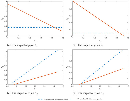
Figure 1.
The impact of μ1 on endurance effort and χ1 on marketing effort under centralized and decentralized decision-making.
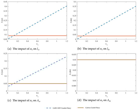
Figure 2.
The impact of α1 on endurance effort and marketing effort under centralized and decentralized decision-making.
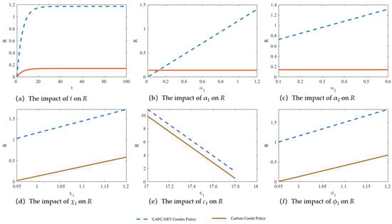
Figure 3.
The impact of t, α1, α2, χ1, c1, and ϕ1 on NEV range increase under decentralized decision-making.
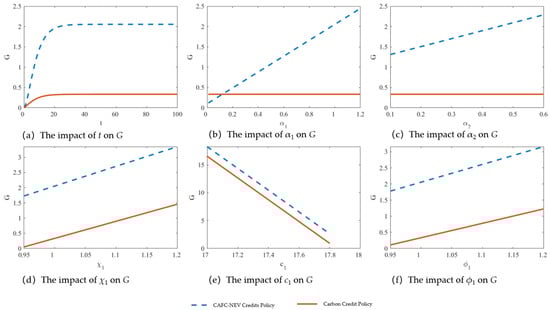
Figure 4.
The impact of t, α1, α2, χ1, c1, and ϕ1 on NEV brand goodwill under decentralized decision-making.
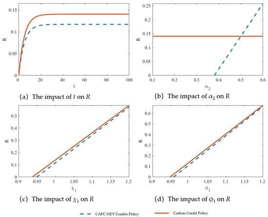
Figure 5.
The impact of t, α2, χ1, and ϕ1 on NEV range increase under decentralized decision-making (α1 = 0.1).
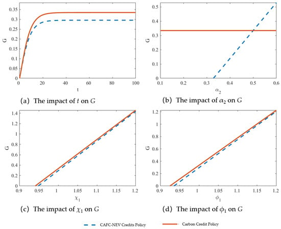
Figure 6.
The impact of t, α2, χ1, and ϕ1 on NEV brand goodwill under decentralized decision-making (α1 = 0.1).
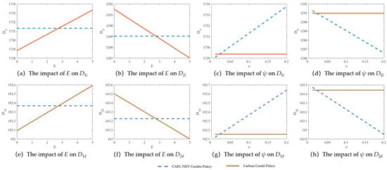
Figure 7.
The impact of E and ψ on the NEV and ICEV demand for dual-channel under decentralized decision-making.
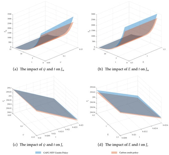
Figure 8.
The impact of ψ, E, and t on the profits of the manufacturer and retailer under CAFC-NEV credits and carbon credits.
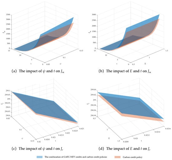
Figure 9.
The impact of ψ, E, and t on the profits of manufacturer and retailer under the combination of CAFC-NEV credits and carbon credit policies and the carbon credit policy.
As shown in Figure 1, when the NEV retail ratio exceeds a certain threshold, regardless of whether it is the CAFC-NEV credits policy or the carbon credit policy, the endurance and marketing efforts under centralized decision-making are higher than those under decentralized decision-making. It may be that the manufacturer and the retailer are independent decision-making subjects in decentralized decision-making, and the manufacturer sets a higher wholesale price for the retail channel in order to maximize its own profit. Retailers then add another markup to form the final retail price, resulting in double marginalization, which makes the final price of the retail channel higher and the sales volume lower, reducing the overall profit of the supply chain and consequently limiting funds available for endurance or marketing. Under centralized decision-making, the system can coordinate the price, endurance and marketing strategies of the dual channel to eliminate the double marginalization. Corollarys 1–4 are verified. Furthermore, Figure 1 also shows that, regardless of whether it is the CAFC-NEV credits policy or the carbon credit policy, the endurance effort decreases as the NEV retail ratio gradually increases, while the marketing effort increases as the impact coefficient of NEV brand goodwill on NEV demand increases.
Figure 2 shows that under the CAFC-NEV credits policy scenario, endurance effort is positively correlated with NEV credit score, while marketing effort is positively correlated with the NEV credit score in the centralized decision-making model but not with NEV credit score in the decentralized decision-making model, consistent with the results of the comparative static analysis. Furthermore, when the NEV credit score is below a certain threshold, the endurance effort under the carbon credit policy is higher than that under the CAFC-NEV credits policy, further validating Corollarys 5–8. Figure 2 demonstrates that as the NEV credit score gradually decreases, implementing a carbon credit policy is more effective for manufacturers’ endurance effort and retailers’ marketing effort.
Figure 3 and Figure 4 illustrate the changes in NEV range increase and brand goodwill with various parameters, respectively. Under the current parameter settings, the range technology will gradually mature and stabilize over time, thus improving the range increase. As shown in Figure 3a, the NEV range increase tends to plateau at t = 30 and beyond. With parameter variations, the NEV range increase and brand goodwill trajectory have some effects consistent with expectations. For example, increases in NEV credit score, required proportion, and the demand coefficient of NEV brand goodwill and range lead to increased range. The change rule of NEV brand goodwill is similar to that of NEV range increase.
From a steady-state perspective, the NEV range increase and brand goodwill under the CAFC-NEV credits policy scenario are higher than those under the carbon credit policy scenario. However, when the NEV credit score is below the threshold, the NEV range increase and brand goodwill under the carbon credit policy scenario will be higher than those under the CAFC-NEV credits policy scenario, as shown in Figure 5 and Figure 6. Corollary 9–Corollary 10 are verified.
Figure 7 illustrates the variation in NEV and ICEV demand with respect to various parameters. It can be seen that, firstly, both CAFC-NEV credits and carbon credit policies can promote NEV consumption demand. As the gains from CAFC-NEV credits or carbon credits increase, the NEV demand rises, while the ICEV demand decreases. Second, if the price of CAFC-NEV credits is lower than or the carbon credit gain is higher than a certain threshold, the implementation of the carbon credit policy is more effective in promoting NEV consumption than the CAFC-NEV credits policy. When the CAFC-NEV credit price is above, or the carbon credit gain is below a specific threshold, the implementation of the carbon credit policy reduces ICEV consumption more than the CAFC-NEV credit policy. Corollarys 11–12 are verified.
Figure 8 shows the difference in manufacturer or retailer profits under the CAFC-NEV credits and carbon credit policy scenarios. Under the parameter configuration plane of Figure 8, the average difference rates of manufacturer profit under the two policy scenarios are 13.130% and 13.129%, respectively, while the average difference rates of retailer profit under the two policy scenarios are 0.003% and 0.002%, respectively. Changes in CAFC-NEV credit price or carbon credit gain will alter the profitability among members under different policies. Therefore, manufacturers and retailers need to consider their own circumstances and the policies to find the optimal way to maximize their profits.
Figure 9 considers the new and old policy transition, that is, the carbon credit policy based on the CAFC-NEV credits policy is implemented for a period of time, and then the CAFC-NEV credits policy is removed. On the parameter configuration plane in Figure 9, if the CAFC-NEV credits policy is canceled after the implementation of the CAFC-NEV credits plus carbon credit policy, the profits of all members in the supply chain change slightly. The profits of the manufacturer decrease by 13.133% and 13.135%, and the profits of the retailer decrease by 0.004% and 0.003%, respectively.
Table 6, Table 7 and Table 8 present the results of the system sensitivity analysis of the NEV credit score (α1), CAFC-NEV credit price (ψ), and carbon credit gain (E), respectively. The results show that the research conclusions are robust across multiple intervals.
Table 6.
Sensitivity analysis of α1 under decentralized decision-making.
Table 7.
Sensitivity analysis of ψ under decentralized decision-making.
Table 8.
Sensitivity analysis of E under decentralized decision-making.
In reality, as a market-based tool to replace the CAFC-NEV credits policy, the carbon credit policy has not yet formed a complete institutional system for its implementation. First, China has not yet established a carbon trading system for the transportation sector at the institutional level, which means that the carbon credit policy lacks the support of higher-level laws and a unified implementation framework, resulting in institutional gaps when the policy is transformed from theoretical conception to actual operation. Second, implementing carbon credit requires accurate statistics and monitoring of actual carbon emissions from NEVs, but current efforts in the statistics, monitoring, and accounting of carbon emissions data still need to be strengthened. Quantifying the contribution of NEV travel to carbon emission reduction and registering them as tradable carbon credits involves complex technical standards and administrative procedures. Third, promoting the marketization of carbon credit trading is a prerequisite for the policy to take effect, but at present, there is a lack of a mature trading platform and price discovery mechanism, making it difficult to guarantee that NEV owners can obtain carbon credit gains in a stable and reasonable manner. In conclusion, the practical application of the carbon credit policy is not simply a technical issue, but rather a systemic institutional problem involving top-level design, accounting, right confirmation, and trading mechanisms. To promote the implementation of the carbon credit policy, it is necessary to address the aforementioned obstacles institutionally, based on the quantitative conclusions of the research.
5. Conclusions and Policy Recommendations
5.1. Conclusions
This paper considers a dual-channel supply chain consisting of a manufacturer and a retailer, capable of simultaneously producing and selling NEVs and ICEVs. The manufacturer is responsible for the production of two types of vehicles and the investment in NEV range technology. The retailer is responsible for marketing and sales. The manufacturer can sell vehicles through retail channels (retailers) and direct sales channels (manufacturer). This paper analyzes the centralized and decentralized decision-making under a dual-channel approach, and further discusses the performance of members under the scenarios of CAFC-NEV credits, carbon credits, and the combination of CAFC-NEV credits and carbon credits. From the analysis and comparison, we draw the following conclusions.
First, some general conclusions are as follows: (1) Regardless of whether the decision-making model is centralized or decentralized, carbon credit has no direct impact on the manufacturer’s endurance effort or the retailer’s marketing effort, but the CAFC-NEV credits policy affects the decisions of the supply chain. The strategies of the combination of CAFC-NEV credits and carbon credit is equivalent to the single CAFC-NEV credits policy. Therefore, implementing a carbon credit policy based on the CAFC-NEV credits policy does not affect the NEV range increase. (2) In decentralized decision-making, the marketing effort under CAFC-NEV credits and carbon credit policies is equal, and the CAFC-NEV credits policy has no incentive effect on the retailer’s marketing effort, while the CAFC-NEV credits policy under centralized decision-making positively incentivize retailer’s marketing effort. (3) Both CAFC-NEV credits and carbon credit policies can promote the NEV development while suppressing the ICEV demand. The higher the policy-related benefits (CAFC-NEV credits price, carbon credit gain), the more obvious the effect on promoting NEV demand and suppressing ICEV demand. (4) The carbon credit policy has a relatively small impact on retailers’ profits, but a larger impact on manufacturers. During the transition from implementing the carbon credit policy on the basis of the CAFC-NEV credits policy to its subsequent cancellation, the profits among supply chain members change slightly.
Second, the conclusions under certain specific conditions are as follows. (1) The superiority or inferiority of decision-making models is not absolute, and the performance difference between centralized and decentralized decision-making is constrained by multiple parameters. (2) In decentralized decision-making, when the NEV credit score is below a certain threshold, the NEV range increase and brand goodwill under the carbon credit policy is higher than that under the CAFC-NEV credits policy, which further increases the NEV demand. This rule also applies in centralized decision-making. (3) When the NEV retail ratio is greater than a certain threshold, regardless of whether it is CAFC-NEV credits or carbon credit policies, the endurance effort and marketing effort in centralized decision-making are higher than those in decentralized decision-making. Meanwhile, the negative impact of the double marginalization of decentralized decision-making on supply chain investment is more prominent. (4) In centralized decision-making, the incentive effects of CAFC-NEV credits and carbon credit policies on retailers’ marketing efforts differ. Due to parameter threshold constraints, the marketing effort under a certain policy may be higher.
5.2. Policy Recommendations
(1) At present, the road transportation sector of China has not established a standardized carbon trading system. The competent authorities should focus on the key aspects to design the NEV carbon credit program, promote pilot demonstrations, strengthen the statistics and monitoring of carbon emission data, promote the marketization of carbon credit trading, reasonably improve the carbon credit gain for NEV owners, so that consumers can effectively enjoy the benefits of the carbon credit policy. We will give full play to the leveraging role of policies on market demand.
(2) It is suggested that the competent authorities, in light of the actual development of the NEV industry, precisely quantify the threshold of NEV credit score for the attenuation of the policy incentive effect of CAFC-NEV credits. When the actual score level approaches or falls below this threshold, the CAFC-NEV credits policy should be promptly abolished, and the scope and coverage of the carbon credit policy should be expanded simultaneously to achieve a smooth transition between the old and new policies.
(3) Our research reveals that implementing carbon credits on the basis of CAFC-NEV credits results in minor fluctuations for supply chain profits, demonstrating the feasibility of policy transition. Therefore, policymakers should design a policy timetable for a smooth transition from CAFC-NEV credits to carbon credits, clarify the exit pace of the CAFC-NEV credits policy and the implementation plan of the carbon credit policy, and stabilize the business expectations of manufacturers and retailers.
5.3. Research Prospects
In summary, this paper draws several conclusions with profound management implications, but these can be extended in various ways. For example, it does not consider the carry-over of credits across years, which has certain limitations. In fact, the newly revised CAFC-NEV credits policy has added NEV credit pool management to balance the supply and demand of credits each year. The modeling treatment of the carbon credit mechanism is highly stylized. Critical institutional features are not incorporated, such as carbon price volatility, transaction costs, enforcement, and interactions with the national ETS. Without engagement with these realities, policy implications risk being overly idealized. In addition, there may be some uncertainties affecting the demand for automobiles. We expect these issues to be addressed in future research.
Author Contributions
Writing—original draft preparation, N.L.; visualization, T.Z., and X.Z.; data curation, S.C., T.Z., and X.Z.; conceptualization, S.C.; methodology, J.K.; writing—review and editing, J.K.; supervision J.K. All authors have read and agreed to the published version of the manuscript.
Funding
This research received no external funding.
Institutional Review Board Statement
Not applicable.
Informed Consent Statement
Not applicable.
Data Availability Statement
The data are contained within the paper.
Conflicts of Interest
The authors declare no conflicts of interest.
Appendix A. The Proof of Proposition 1–6
Proof of Proposition 1.
According to optimal control theory, the optimal value function of the manufacturer’s and retailer’s profits at time t is given by
For any R ≥ 0 and G ≥ 0, VD(R,G) satisfies the Hamilton–Jacobi–Bellman function as
Equation (A2) is a concave function with respect to I(t) and A(t).
The necessary conditions for the optimal strategies of Equation (A2) is given by
we obtain
By substituting Equations (A3) and (A4) into (A2), we obtain
According to Equation (A5), we assume ρVD(R,G) is a linear function of R and G.
where , , are unknown constants.
By substituting Equation (A6) into (A5), we obtain
If p1i = p1d, p2i = p2d (the same below). Substituting Equations (A7) into (A3) and (A4), respectively, yields optimal equilibrium strategies shown in (34) and (35). □
Proof of Proposition 2.
According to optimal control theory, the optimal value function of the manufacturer’s and retailer’s profits at time t is given by
For any R ≥ 0 and G ≥ 0, VC(R,G) satisfies the Hamilton–Jacobi–Bellman function as
Equation (A9) is a concave function with respect to I(t) and A(t).
The necessary conditions for the optimal strategies of Equation (A9) is given by
we obtain
By substituting Equations (A10) and (A11) into (A9), we obtain
According to Equation (A5), we assume ρVC(R,G) is a linear function of R and G.
where , , are unknown constants.
By substituting Equation (A13) into (A12), we obtain
Substituting Equations (A14) into (A10) and (A11), respectively, yields optimal equilibrium strategies shown in (44) and (45). □
Proof of Proposition 3.
According to optimal control theory, the optimal value function of the manufacturer’s and retailer’s profits at time t is given by
For any R ≥ 0 and G ≥ 0, VCD(R,G) satisfies the Hamilton–Jacobi–Bellman function as
Equation (A16) is a concave function with respect to I(t) and A(t).
The necessary conditions for the optimal strategies of Equation (A16) are given by
we obtain
By substituting Equations (A17) and (A18) into (A16), we obtain
According to Equation (A19), we assume ρVCD(R,G) is a linear function of R and G.
where , , and are unknown constants.
By substituting Equation (A20) into (A19), we obtain
Substituting Equations (A21) into (A17) and (A18), respectively, yields optimal equilibrium strategies shown in (54) and (55). □
Proof of Proposition 4.
According to optimal control theory, the optimal value function of the manufacturer and retailer’s profits at time t is given by
For any R ≥ 0 and G ≥ 0, (R,G) and (R,G) satisfy the Hamilton–Jacobi–Bellman function as
Equations (A24) and (A25) are concave functions with respect to I(t) and A(t), respectively.
The necessary conditions for the optimal strategies of Equation (A24) are given by
The necessary conditions for the optimal strategies of Equation (A25) are given by
we obtain
By substituting Equations (A26) and (A27) into (A24) and (A25), we obtain
According to Equations (A28) and (A29), we assume (R,G) and (R,G) are linear functions of R and G.
where , , , , , are unknown constants.
By substituting Equations (A9) into (A7) and (A8), we obtain
Substituting Equations (A31) and (A32) into (A26) and (A27), respectively, yields optimal equilibrium strategies shown in (64) and (65). □
Proof of Proposition 5.
According to optimal control theory, the optimal value function of the manufacturer and retailer’s profits at time t is given by
For any R ≥ 0 and G ≥ 0, (R,G) and (R,G) satisfy the Hamilton–Jacobi–Bellman function as
Equations (A35) and (A36) are concave functions with respect to I(t) and A(t), respectively.
The necessary conditions for the optimal strategies of Equation (A35) are given by
The necessary conditions for the optimal strategies of Equation (A36) are given by
we obtain
By substituting Equations (A37) and (A38) into (A35) and (A36), we obtain
According to Equations (A39) and (A40), we assume (R,G) and (R,G) are linear functions of R and G.
where , , , , , are unknown constants.
By substituting Equations (A41) into (A39) and (A40), we obtain
Substituting Equations (A42) and (A43) into (A37) and (A38), respectively, yields optimal equilibrium strategies shown in (78) and (79). □
Proof of Proposition 6.
According to optimal control theory, the optimal value function of the manufacturer and retailer’s profits at time t is given by
For any R ≥ 0 and G ≥ 0, (R,G) and (R,G) satisfy the Hamilton–Jacobi–Bellman function as
Equations (A46) and (A47) are concave functions with respect to I(t) and A(t), respectively.
The necessary conditions for the optimal strategies of Equation (A46) is given by
The necessary conditions for the optimal strategies of Equation (A47) is given by
we obtain
By substituting Equations (A48) and (A49) into (A46) and (A47), we obtain
According to Equations (A50) and (A51), we assume (R,G) and (R,G) are linear functions of R and G.
where , , , , , are unknown constants.
By substituting Equations (A52) into (A50) and (A51), we obtain
Substituting Equations (A53) and (A54) into (A48) and (A49), respectively, yields optimal equilibrium strategies shown in (92) and (93).
The state equations are given by Assumptions 1 and 2, and have the same form in all policy scenarios; therefore, the Jacobian matrix and stability conditions of the system are also the same. We can write the state equations in matrix form.
This is a linear nonhomogeneous system , where J is the Jacobian matrix of the system. For a linear system, the Jacobian matrix is simply the coefficient matrix J.
The stability of the linear system is determined by the stability of the homogeneous system, that is, by the eigenvalues of J.
The eigenvalues λ satisfy the characteristic equation: , i.e.,:
The eigenvalues are λ1 = −δR and λ2 = = −δG. According to the model assumptions, δR > 0 and δG > 0, satisfying the stability condition that the real parts of all eigenvalues are negative. Therefore, the system is globally asymptotically stable at the equilibrium point (R*, G*). □
Appendix B. Sensitivity Analysis
Table A1.
Sensitivity analysis of β1 under decentralized decision-making.
Table A1.
Sensitivity analysis of β1 under decentralized decision-making.
| β1 = 0.1 | β1 = 0.5 | β1 = 1 | β1 = 5 | β1 = 10 | β1 = 15 | β1 = 20 | β1 = 25 | β1 = 30 | β1 = 35 | |
|---|---|---|---|---|---|---|---|---|---|---|
| 0.29 | 0.29 | 0.29 | 0.29 | 0.29 | 0.29 | 0.29 | 0.29 | 0.29 | 0.29 | |
| 0.03 | 0.03 | 0.03 | 0.03 | 0.03 | 0.03 | 0.03 | 0.03 | 0.03 | 0.03 | |
| 1830.03 | 1823.34 | 1814.98 | 1748.05 | 1664.40 | 1580.74 | 1497.09 | 1413.43 | 1329.78 | 1246.12 | |
| 203.34 | 202.59 | 201.66 | 194.23 | 184.93 | 175.64 | 166.34 | 157.05 | 147.75 | 138.46 | |
| 1289.04 | 1289.04 | 1289.04 | 1289.04 | 1289.04 | 1289.04 | 1289.04 | 1289.04 | 1289.04 | 1289.04 | |
| 143.23 | 143.23 | 143.23 | 143.23 | 143.23 | 143.23 | 143.23 | 143.23 | 143.23 | 143.23 | |
| 1.17 | 1.17 | 1.17 | 1.17 | 1.17 | 1.17 | 1.17 | 1.17 | 1.17 | 1.17 | |
| 2.06 | 2.06 | 2.06 | 2.06 | 2.06 | 2.06 | 2.06 | 2.06 | 2.06 | 2.06 | |
| 5505.67 | 5492.83 | 5476.78 | 5348.38 | 5187.89 | 5027.40 | 4866.90 | 4706.41 | 4545.91 | 4385.42 | |
| 3864.75 | 3856.28 | 3845.68 | 3760.91 | 3654.95 | 3548.98 | 3443.02 | 3337.06 | 3231.10 | 3125.13 | |
| 0.04 | 0.04 | 0.04 | 0.04 | 0.04 | 0.04 | 0.04 | 0.04 | 0.04 | 0.04 | |
| 0.03 | 0.03 | 0.03 | 0.03 | 0.03 | 0.03 | 0.03 | 0.03 | 0.03 | 0.03 | |
| 1828.09 | 1821.40 | 1813.04 | 1746.11 | 1662.46 | 1578.80 | 1495.15 | 1411.49 | 1327.84 | 1244.18 | |
| 203.12 | 202.38 | 201.45 | 194.01 | 184.72 | 175.42 | 166.13 | 156.83 | 147.54 | 138.24 | |
| 1290.98 | 1290.98 | 1290.98 | 1290.98 | 1290.98 | 1290.98 | 1290.98 | 1290.98 | 1290.98 | 1290.98 | |
| 143.44 | 143.44 | 143.44 | 143.44 | 143.44 | 143.44 | 143.44 | 143.44 | 143.44 | 143.44 | |
| 0.14 | 0.14 | 0.14 | 0.14 | 0.14 | 0.14 | 0.14 | 0.14 | 0.14 | 0.14 | |
| 0.33 | 0.33 | 0.33 | 0.33 | 0.33 | 0.33 | 0.33 | 0.33 | 0.33 | 0.33 | |
| 4771.40 | 4761.04 | 4748.09 | 4644.48 | 4514.97 | 4385.46 | 4255.95 | 4126.44 | 3996.93 | 3867.42 | |
| 3864.74 | 3856.27 | 3845.67 | 3760.90 | 3654.94 | 3548.97 | 3443.01 | 3337.05 | 3231.09 | 3125.12 |
Table A2.
Sensitivity Analysis of β2 under Decentralized Decision-making.
Table A2.
Sensitivity Analysis of β2 under Decentralized Decision-making.
| β2 = 0.1 | β2 = 0.5 | β2 = 1 | β2 = 5 | β2 = 10 | β2 = 15 | β2 = 20 | β2 = 25 | β2 = 30 | β2 = 35 | |
|---|---|---|---|---|---|---|---|---|---|---|
| 0.29 | 0.29 | 0.29 | 0.29 | 0.29 | 0.29 | 0.29 | 0.29 | 0.29 | 0.29 | |
| 0.03 | 0.03 | 0.03 | 0.03 | 0.03 | 0.03 | 0.03 | 0.03 | 0.03 | 0.03 | |
| 1731.32 | 1731.32 | 1731.32 | 1731.32 | 1731.32 | 1731.32 | 1731.32 | 1731.32 | 1731.32 | 1731.32 | |
| 192.37 | 192.37 | 192.37 | 192.37 | 192.37 | 192.37 | 192.37 | 192.37 | 192.37 | 192.37 | |
| 1766.70 | 1760.31 | 1752.32 | 1688.42 | 1608.54 | 1528.67 | 1448.79 | 1368.92 | 1289.04 | 1209.17 | |
| 196.30 | 195.59 | 194.70 | 187.60 | 178.73 | 169.85 | 160.98 | 152.10 | 143.23 | 134.35 | |
| 1.17 | 1.17 | 1.17 | 1.17 | 1.17 | 1.17 | 1.17 | 1.17 | 1.17 | 1.17 | |
| 2.06 | 2.06 | 2.06 | 2.06 | 2.06 | 2.06 | 2.06 | 2.06 | 2.06 | 2.06 | |
| 6055.76 | 6045.87 | 6033.50 | 5934.58 | 5810.92 | 5687.26 | 5563.60 | 5439.94 | 5316.28 | 5192.63 | |
| 4312.90 | 4305.23 | 4295.65 | 4218.97 | 4123.12 | 4027.27 | 3931.42 | 3835.57 | 3739.72 | 3643.87 | |
| 0.04 | 0.04 | 0.04 | 0.04 | 0.04 | 0.04 | 0.04 | 0.04 | 0.04 | 0.04 | |
| 0.03 | 0.03 | 0.03 | 0.03 | 0.03 | 0.03 | 0.03 | 0.03 | 0.03 | 0.03 | |
| 1729.38 | 1729.38 | 1729.38 | 1729.38 | 1729.38 | 1729.38 | 1729.38 | 1729.38 | 1729.38 | 1729.38 | |
| 192.15 | 192.15 | 192.15 | 192.15 | 192.15 | 192.15 | 192.15 | 192.15 | 192.15 | 192.15 | |
| 1768.63 | 1762.24 | 1754.26 | 1690.36 | 1610.48 | 1530.61 | 1450.73 | 1370.86 | 1290.98 | 1211.11 | |
| 196.51 | 195.80 | 194.92 | 187.82 | 178.94 | 170.07 | 161.19 | 152.32 | 143.44 | 134.57 | |
| 0.14 | 0.14 | 0.14 | 0.14 | 0.14 | 0.14 | 0.14 | 0.14 | 0.14 | 0.14 | |
| 0.33 | 0.33 | 0.33 | 0.33 | 0.33 | 0.33 | 0.33 | 0.33 | 0.33 | 0.33 | |
| 5336.83 | 5327.22 | 5315.21 | 5219.12 | 5099.01 | 4978.90 | 4858.80 | 4738.69 | 4618.58 | 4498.47 | |
| 4312.89 | 4305.22 | 4295.64 | 4218.96 | 4123.11 | 4027.26 | 3931.41 | 3835.56 | 3739.71 | 3643.86 |
Table A3.
Sensitivity analysis of χ1 under decentralized decision-making.
Table A3.
Sensitivity analysis of χ1 under decentralized decision-making.
| χ1 = 0.1 | χ1 = 0.3 | χ1 = 0.5 | χ1 = 0.7 | χ1 = 0.9 | χ1 = 1.1 | χ1 = 1.3 | χ1 = 1.5 | χ1 = 1.7 | χ1 = 1.9 | |
|---|---|---|---|---|---|---|---|---|---|---|
| −0.33 | −0.19 | −0.05 | 0.09 | 0.22 | 0.36 | 0.50 | 0.64 | 0.78 | 0.91 | |
| −0.48 | −0.37 | −0.26 | −0.14 | −0.03 | 0.09 | 0.20 | 0.32 | 0.43 | 0.54 | |
| 1726.89 | 1727.06 | 1727.69 | 1728.79 | 1730.36 | 1732.40 | 1734.90 | 1737.88 | 1741.32 | 1745.23 | |
| 191.88 | 191.90 | 191.97 | 192.09 | 192.26 | 192.49 | 192.77 | 193.10 | 193.48 | 193.91 | |
| 1296.55 | 1294.88 | 1293.21 | 1291.55 | 1289.88 | 1288.21 | 1286.54 | 1284.87 | 1283.21 | 1281.54 | |
| 144.06 | 143.88 | 143.69 | 143.51 | 143.32 | 143.13 | 142.95 | 142.76 | 142.58 | 142.39 | |
| −1.31 | −0.76 | −0.21 | 0.34 | 0.90 | 1.45 | 2.00 | 2.55 | 3.11 | 3.66 | |
| −3.80 | −2.50 | −1.20 | 0.10 | 1.41 | 2.71 | 4.01 | 5.31 | 6.61 | 7.91 | |
| 5317.29 | 5316.72 | 5316.35 | 5316.18 | 5316.20 | 5316.42 | 5316.83 | 5317.43 | 5318.23 | 5319.23 | |
| 3740.44 | 3740.06 | 3739.80 | 3739.67 | 3739.67 | 3739.80 | 3740.05 | 3740.43 | 3740.93 | 3741.57 | |
| −0.47 | −0.35 | −0.24 | −0.13 | −0.02 | 0.09 | 0.20 | 0.31 | 0.43 | 0.54 | |
| −0.48 | −0.37 | −0.26 | −0.14 | −0.03 | 0.09 | 0.20 | 0.32 | 0.43 | 0.54 | |
| 1726.85 | 1726.71 | 1726.96 | 1727.63 | 1728.70 | 1730.17 | 1732.05 | 1734.33 | 1737.01 | 1740.10 | |
| 191.87 | 191.86 | 191.88 | 191.96 | 192.08 | 192.24 | 192.45 | 192.70 | 193.00 | 193.34 | |
| 1297.34 | 1295.92 | 1294.51 | 1293.10 | 1291.69 | 1290.28 | 1288.86 | 1287.45 | 1286.04 | 1284.63 | |
| 144.15 | 143.99 | 143.83 | 143.68 | 143.52 | 143.36 | 143.21 | 143.05 | 142.89 | 142.74 | |
| −1.87 | −1.42 | −0.97 | −0.53 | −0.08 | 0.36 | 0.81 | 1.26 | 1.70 | 2.15 | |
| −4.72 | −3.60 | −2.47 | −1.35 | −0.23 | 0.90 | 2.02 | 3.14 | 4.27 | 5.39 | |
| 4619.91 | 4619.36 | 4618.95 | 4618.69 | 4618.58 | 4618.61 | 4618.80 | 4619.13 | 4619.60 | 4620.23 | |
| 3740.65 | 3740.24 | 3739.95 | 3739.77 | 3739.70 | 3739.74 | 3739.90 | 3740.16 | 3740.53 | 3741.02 |
Table A4.
Sensitivity analysis of χ2 under decentralized decision-making.
Table A4.
Sensitivity analysis of χ2 under decentralized decision-making.
| χ2 = 0.1 | χ2 = 0.3 | χ2 = 0.5 | χ2 = 0.7 | χ2 = 0.9 | χ2 = 1.1 | χ2 = 1.3 | χ2 = 1.5 | χ2 = 1.7 | χ2 = 1.9 | |
|---|---|---|---|---|---|---|---|---|---|---|
| 0.79 | 0.68 | 0.57 | 0.46 | 0.35 | 0.24 | 0.13 | 0.01 | −0.10 | −0.21 | |
| 0.52 | 0.41 | 0.30 | 0.19 | 0.08 | −0.02 | −0.13 | −0.24 | −0.35 | −0.46 | |
| 1737.59 | 1736.20 | 1734.81 | 1733.41 | 1732.02 | 1730.62 | 1729.23 | 1727.83 | 1726.44 | 1725.05 | |
| 193.07 | 192.91 | 192.76 | 192.60 | 192.45 | 192.29 | 192.14 | 191.98 | 191.83 | 191.67 | |
| 1288.46 | 1287.89 | 1287.72 | 1287.95 | 1288.58 | 1289.61 | 1291.03 | 1292.85 | 1295.06 | 1297.67 | |
| 143.16 | 143.10 | 143.08 | 143.11 | 143.18 | 143.29 | 143.45 | 143.65 | 143.90 | 144.19 | |
| 3.18 | 2.73 | 2.29 | 1.84 | 1.40 | 0.95 | 0.50 | 0.06 | −0.39 | −0.83 | |
| 7.02 | 5.92 | 4.81 | 3.71 | 2.61 | 1.50 | 0.40 | −0.70 | −1.81 | −2.91 | |
| 5318.54 | 5317.79 | 5317.18 | 5316.72 | 5316.39 | 5316.21 | 5316.17 | 5316.27 | 5316.51 | 5316.90 | |
| 3741.28 | 3740.75 | 3740.33 | 3740.01 | 3739.79 | 3739.67 | 3739.66 | 3739.75 | 3739.95 | 3740.24 | |
| 0.52 | 0.41 | 0.31 | 0.20 | 0.09 | −0.02 | −0.13 | −0.24 | −0.34 | −0.45 | |
| 0.52 | 0.41 | 0.30 | 0.19 | 0.08 | −0.02 | −0.13 | −0.24 | −0.35 | −0.46 | |
| 1735.52 | 1734.15 | 1732.79 | 1731.43 | 1730.06 | 1728.70 | 1727.34 | 1725.97 | 1724.61 | 1723.25 | |
| 192.84 | 192.68 | 192.53 | 192.38 | 192.23 | 192.08 | 191.93 | 191.77 | 191.62 | 191.47 | |
| 1289.06 | 1288.81 | 1288.94 | 1289.47 | 1290.38 | 1291.68 | 1293.37 | 1295.46 | 1297.93 | 1300.79 | |
| 143.23 | 143.20 | 143.22 | 143.27 | 143.38 | 143.52 | 143.71 | 143.94 | 144.21 | 144.53 | |
| 2.09 | 1.66 | 1.22 | 0.79 | 0.36 | −0.08 | −0.51 | −0.94 | −1.37 | −1.81 | |
| 5.20 | 4.12 | 3.04 | 1.96 | 0.88 | −0.21 | −1.29 | −2.37 | −3.45 | −4.53 | |
| 4620.11 | 4619.53 | 4619.09 | 4618.78 | 4618.61 | 4618.58 | 4618.68 | 4618.92 | 4619.30 | 4619.81 | |
| 3740.91 | 3740.47 | 3740.12 | 3739.88 | 3739.74 | 3739.70 | 3739.76 | 3739.92 | 3740.19 | 3740.55 |
Table A5.
Sensitivity analysis of ϕ1 under decentralized decision-making.
Table A5.
Sensitivity analysis of ϕ1 under decentralized decision-making.
| ϕ1 = 0.1 | ϕ1 = 0.3 | ϕ1 = 0.5 | ϕ1 = 0.7 | ϕ1 = 0.9 | ϕ1 = 1.1 | ϕ1 = 1.3 | ϕ1 = 1.5 | ϕ1 = 1.7 | ϕ1 = 1.9 | |
|---|---|---|---|---|---|---|---|---|---|---|
| −0.45 | −0.29 | −0.12 | 0.04 | 0.21 | 0.38 | 0.54 | 0.71 | 0.87 | 1.04 | |
| 0.03 | 0.03 | 0.03 | 0.03 | 0.03 | 0.03 | 0.03 | 0.03 | 0.03 | 0.03 | |
| 1725.63 | 1726.47 | 1727.56 | 1728.88 | 1730.45 | 1732.25 | 1734.29 | 1736.57 | 1739.09 | 1741.85 | |
| 191.74 | 191.83 | 191.95 | 192.10 | 192.27 | 192.47 | 192.70 | 192.95 | 193.23 | 193.54 | |
| 1296.20 | 1294.61 | 1293.02 | 1291.43 | 1289.84 | 1288.25 | 1286.66 | 1285.07 | 1283.47 | 1281.88 | |
| 144.02 | 143.85 | 143.67 | 143.49 | 143.32 | 143.14 | 142.96 | 142.79 | 142.61 | 142.43 | |
| −1.81 | −1.15 | −0.48 | 0.18 | 0.84 | 1.50 | 2.17 | 2.83 | 3.49 | 4.16 | |
| −2.92 | −1.81 | −0.71 | 0.40 | 1.50 | 2.61 | 3.71 | 4.82 | 5.92 | 7.03 | |
| 5316.48 | 5316.28 | 5316.17 | 5316.14 | 5316.21 | 5316.38 | 5316.63 | 5316.98 | 5317.41 | 5317.94 | |
| 3740.33 | 3739.98 | 3739.76 | 3739.65 | 3739.66 | 3739.80 | 3740.06 | 3740.44 | 3740.93 | 3741.55 | |
| −0.57 | −0.43 | −0.30 | −0.17 | −0.03 | 0.10 | 0.24 | 0.37 | 0.50 | 0.64 | |
| 0.03 | 0.03 | 0.03 | 0.03 | 0.03 | 0.03 | 0.03 | 0.03 | 0.03 | 0.03 | |
| 1725.44 | 1725.98 | 1726.71 | 1727.63 | 1728.75 | 1730.06 | 1731.56 | 1733.26 | 1735.14 | 1737.22 | |
| 191.72 | 191.78 | 191.86 | 191.96 | 192.08 | 192.23 | 192.40 | 192.58 | 192.79 | 193.02 | |
| 1296.76 | 1295.48 | 1294.19 | 1292.91 | 1291.62 | 1290.34 | 1289.06 | 1287.77 | 1286.49 | 1285.20 | |
| 144.08 | 143.94 | 143.80 | 143.66 | 143.51 | 143.37 | 143.23 | 143.09 | 142.94 | 142.80 | |
| −2.27 | −1.73 | −1.20 | −0.66 | −0.13 | 0.41 | 0.94 | 1.48 | 2.01 | 2.55 | |
| −3.68 | −2.79 | −1.89 | −1.00 | −0.11 | 0.78 | 1.67 | 2.56 | 3.46 | 4.35 | |
| 4619.11 | 4618.89 | 4618.73 | 4618.62 | 4618.58 | 4618.59 | 4618.67 | 4618.80 | 4619.00 | 4619.25 | |
| 3740.53 | 3740.18 | 3739.92 | 3739.76 | 3739.70 | 3739.74 | 3739.87 | 3740.10 | 3740.43 | 3740.86 |
Table A6.
Sensitivity analysis of ϕ2 under decentralized decision-making.
Table A6.
Sensitivity analysis of ϕ2 under decentralized decision-making.
| ϕ2 = 0.1 | ϕ2 = 0.3 | ϕ2 = 0.5 | ϕ2 = 0.7 | ϕ2 = 0.9 | ϕ2 = 1.1 | ϕ2 = 1.3 | ϕ2 = 1.5 | ϕ2 = 1.7 | ϕ2 = 1.9 | |
|---|---|---|---|---|---|---|---|---|---|---|
| 0.90 | 0.76 | 0.63 | 0.49 | 0.36 | 0.23 | 0.09 | −0.04 | −0.17 | −0.31 | |
| 0.03 | 0.03 | 0.03 | 0.03 | 0.03 | 0.03 | 0.03 | 0.03 | 0.03 | 0.03 | |
| 1737.10 | 1735.81 | 1734.53 | 1733.25 | 1731.96 | 1730.68 | 1729.39 | 1728.11 | 1726.83 | 1725.54 | |
| 193.01 | 192.87 | 192.73 | 192.58 | 192.44 | 192.30 | 192.15 | 192.01 | 191.87 | 191.73 | |
| 1286.17 | 1286.47 | 1286.96 | 1287.65 | 1288.53 | 1289.60 | 1290.87 | 1292.33 | 1293.98 | 1295.82 | |
| 142.91 | 142.94 | 143.00 | 143.07 | 143.17 | 143.29 | 143.43 | 143.59 | 143.78 | 143.98 | |
| 3.58 | 3.05 | 2.51 | 1.98 | 1.44 | 0.91 | 0.37 | −0.16 | −0.70 | −1.23 | |
| 6.07 | 5.18 | 4.28 | 3.39 | 2.50 | 1.61 | 0.72 | −0.17 | −1.07 | −1.96 | |
| 5317.48 | 5317.11 | 5316.80 | 5316.55 | 5316.36 | 5316.23 | 5316.16 | 5316.14 | 5316.19 | 5316.30 | |
| 3741.22 | 3740.72 | 3740.32 | 3740.01 | 3739.79 | 3739.67 | 3739.63 | 3739.69 | 3739.85 | 3740.09 | |
| 0.62 | 0.49 | 0.36 | 0.23 | 0.10 | −0.03 | −0.16 | −0.29 | −0.42 | −0.55 | |
| 0.03 | 0.03 | 0.03 | 0.03 | 0.03 | 0.03 | 0.03 | 0.03 | 0.03 | 0.03 | |
| 1734.99 | 1733.75 | 1732.50 | 1731.25 | 1730.01 | 1728.76 | 1727.51 | 1726.26 | 1725.02 | 1723.77 | |
| 192.78 | 192.64 | 192.50 | 192.36 | 192.22 | 192.08 | 191.95 | 191.81 | 191.67 | 191.53 | |
| 1287.38 | 1287.85 | 1288.51 | 1289.36 | 1290.39 | 1291.62 | 1293.03 | 1294.62 | 1296.40 | 1298.37 | |
| 143.04 | 143.09 | 143.17 | 143.26 | 143.38 | 143.51 | 143.67 | 143.85 | 144.04 | 144.26 | |
| 2.48 | 1.96 | 1.44 | 0.92 | 0.40 | −0.12 | −0.64 | −1.16 | −1.68 | −2.20 | |
| 4.23 | 3.37 | 2.50 | 1.63 | 0.77 | −0.10 | −0.96 | −1.83 | −2.70 | −3.56 | |
| 4619.22 | 4618.98 | 4618.79 | 4618.67 | 4618.59 | 4618.58 | 4618.62 | 4618.72 | 4618.87 | 4619.08 | |
| 3740.77 | 3740.38 | 3740.08 | 3739.86 | 3739.74 | 3739.70 | 3739.76 | 3739.90 | 3740.14 | 3740.46 |
Table A7.
Sensitivity analysis of γ1 under decentralized decision-making.
Table A7.
Sensitivity analysis of γ1 under decentralized decision-making.
| γ1 = 0.1 | γ1 = 0.3 | γ1 = 0.5 | γ1 = 0.7 | γ1 = 0.9 | γ1 = 1.1 | γ1 = 1.3 | γ1 = 1.5 | γ1 = 1.7 | γ1 = 1.9 | |
|---|---|---|---|---|---|---|---|---|---|---|
| 0.29 | 0.29 | 0.29 | 0.29 | 0.29 | 0.29 | 0.29 | 0.29 | 0.29 | 0.29 | |
| 0.03 | 0.03 | 0.03 | 0.03 | 0.03 | 0.03 | 0.03 | 0.03 | 0.03 | 0.03 | |
| 1731.32 | 1731.32 | 1731.32 | 1731.32 | 1731.32 | 1731.32 | 1731.32 | 1731.32 | 1731.32 | 1731.32 | |
| 192.37 | 192.37 | 192.37 | 192.37 | 192.37 | 192.37 | 192.37 | 192.37 | 192.37 | 192.37 | |
| 1289.04 | 1289.04 | 1289.04 | 1289.04 | 1289.04 | 1289.04 | 1289.04 | 1289.04 | 1289.04 | 1289.04 | |
| 143.23 | 143.23 | 143.23 | 143.23 | 143.23 | 143.23 | 143.23 | 143.23 | 143.23 | 143.23 | |
| 1.17 | 1.17 | 1.17 | 1.17 | 1.17 | 1.17 | 1.17 | 1.17 | 1.17 | 1.17 | |
| 2.06 | 2.06 | 2.06 | 2.06 | 2.06 | 2.06 | 2.06 | 2.06 | 2.06 | 2.06 | |
| 5316.28 | 5316.28 | 5316.28 | 5316.28 | 5316.28 | 5316.28 | 5316.28 | 5316.28 | 5316.28 | 5316.28 | |
| 3739.72 | 3739.72 | 3739.72 | 3739.72 | 3739.72 | 3739.72 | 3739.72 | 3739.72 | 3739.72 | 3739.72 | |
| 0.04 | 0.04 | 0.04 | 0.04 | 0.04 | 0.04 | 0.04 | 0.04 | 0.04 | 0.04 | |
| 0.03 | 0.03 | 0.03 | 0.03 | 0.03 | 0.03 | 0.03 | 0.03 | 0.03 | 0.03 | |
| 1728.90 | 1729.00 | 1729.11 | 1729.22 | 1729.33 | 1729.44 | 1729.54 | 1729.65 | 1729.76 | 1729.87 | |
| 192.10 | 192.11 | 192.12 | 192.14 | 192.15 | 192.16 | 192.17 | 192.18 | 192.20 | 192.21 | |
| 1290.98 | 1290.98 | 1290.98 | 1290.98 | 1290.98 | 1290.98 | 1290.98 | 1290.98 | 1290.98 | 1290.98 | |
| 143.44 | 143.44 | 143.44 | 143.44 | 143.44 | 143.44 | 143.44 | 143.44 | 143.44 | 143.44 | |
| 0.14 | 0.14 | 0.14 | 0.14 | 0.14 | 0.14 | 0.14 | 0.14 | 0.14 | 0.14 | |
| 0.33 | 0.33 | 0.33 | 0.33 | 0.33 | 0.33 | 0.33 | 0.33 | 0.33 | 0.33 | |
| 4617.83 | 4617.99 | 4618.16 | 4618.33 | 4618.50 | 4618.66 | 4618.83 | 4619.00 | 4619.16 | 4619.33 | |
| 3739.09 | 3739.23 | 3739.37 | 3739.50 | 3739.64 | 3739.78 | 3739.91 | 3740.05 | 3740.19 | 3740.32 |
Table A8.
Sensitivity analysis of γ2 under decentralized decision-making.
Table A8.
Sensitivity analysis of γ2 under decentralized decision-making.
| γ2 = 0.1 | γ2 = 0.3 | γ2 = 0.5 | γ2 = 0.7 | γ2 = 0.9 | γ2 = 1.1 | γ2 = 1.3 | γ2 = 1.5 | γ2 = 1.7 | γ2 = 1.9 | |
|---|---|---|---|---|---|---|---|---|---|---|
| 0.29 | 0.29 | 0.29 | 0.29 | 0.29 | 0.29 | 0.29 | 0.29 | 0.29 | 0.29 | |
| 0.03 | 0.03 | 0.03 | 0.03 | 0.03 | 0.03 | 0.03 | 0.03 | 0.03 | 0.03 | |
| 1731.32 | 1731.32 | 1731.32 | 1731.32 | 1731.32 | 1731.32 | 1731.32 | 1731.32 | 1731.32 | 1731.32 | |
| 192.37 | 192.37 | 192.37 | 192.37 | 192.37 | 192.37 | 192.37 | 192.37 | 192.37 | 192.37 | |
| 1289.04 | 1289.04 | 1289.04 | 1289.04 | 1289.04 | 1289.04 | 1289.04 | 1289.04 | 1289.04 | 1289.04 | |
| 143.23 | 143.23 | 143.23 | 143.23 | 143.23 | 143.23 | 143.23 | 143.23 | 143.23 | 143.23 | |
| 1.17 | 1.17 | 1.17 | 1.17 | 1.17 | 1.17 | 1.17 | 1.17 | 1.17 | 1.17 | |
| 2.06 | 2.06 | 2.06 | 2.06 | 2.06 | 2.06 | 2.06 | 2.06 | 2.06 | 2.06 | |
| 5316.28 | 5316.28 | 5316.28 | 5316.28 | 5316.28 | 5316.28 | 5316.28 | 5316.28 | 5316.28 | 5316.28 | |
| 3739.72 | 3739.72 | 3739.72 | 3739.72 | 3739.72 | 3739.72 | 3739.72 | 3739.72 | 3739.72 | 3739.72 | |
| 0.04 | 0.04 | 0.04 | 0.04 | 0.04 | 0.04 | 0.04 | 0.04 | 0.04 | 0.04 | |
| 0.03 | 0.03 | 0.03 | 0.03 | 0.03 | 0.03 | 0.03 | 0.03 | 0.03 | 0.03 | |
| 1729.38 | 1729.38 | 1729.38 | 1729.38 | 1729.38 | 1729.38 | 1729.38 | 1729.38 | 1729.38 | 1729.38 | |
| 192.15 | 192.15 | 192.15 | 192.15 | 192.15 | 192.15 | 192.15 | 192.15 | 192.15 | 192.15 | |
| 1291.47 | 1291.36 | 1291.25 | 1291.14 | 1291.04 | 1290.93 | 1290.82 | 1290.71 | 1290.60 | 1290.50 | |
| 143.50 | 143.48 | 143.47 | 143.46 | 143.45 | 143.44 | 143.42 | 143.41 | 143.40 | 143.39 | |
| 0.14 | 0.14 | 0.14 | 0.14 | 0.14 | 0.14 | 0.14 | 0.14 | 0.14 | 0.14 | |
| 0.33 | 0.33 | 0.33 | 0.33 | 0.33 | 0.33 | 0.33 | 0.33 | 0.33 | 0.33 | |
| 4619.31 | 4619.15 | 4618.98 | 4618.82 | 4618.66 | 4618.50 | 4618.34 | 4618.17 | 4618.01 | 4617.85 | |
| 3740.29 | 3740.16 | 3740.03 | 3739.90 | 3739.77 | 3739.64 | 3739.51 | 3739.38 | 3739.25 | 3739.12 |
Table A9.
Sensitivity analysis of β1 under centralized decision-making.
Table A9.
Sensitivity analysis of β1 under centralized decision-making.
| β1 = 0.1 | β1 = 0.5 | β1 = 1 | β1 = 5 | β1 = 10 | β1 = 15 | β1 = 20 | β1 = 25 | β1 = 30 | β1 = 35 | |
|---|---|---|---|---|---|---|---|---|---|---|
| 0.35 | 0.35 | 0.35 | 0.35 | 0.35 | 0.35 | 0.35 | 0.35 | 0.35 | 0.35 | |
| 0.20 | 0.20 | 0.20 | 0.20 | 0.20 | 0.20 | 0.20 | 0.20 | 0.20 | 0.20 | |
| 1831.04 | 1824.35 | 1815.98 | 1749.06 | 1665.40 | 1581.75 | 1498.09 | 1414.44 | 1330.78 | 1247.13 | |
| 203.45 | 202.71 | 201.78 | 194.34 | 185.04 | 175.75 | 166.45 | 157.16 | 147.86 | 138.57 | |
| 1288.04 | 1288.04 | 1288.04 | 1288.04 | 1288.04 | 1288.04 | 1288.04 | 1288.04 | 1288.04 | 1288.04 | |
| 143.12 | 143.12 | 143.12 | 143.12 | 143.12 | 143.12 | 143.12 | 143.12 | 143.12 | 143.12 | |
| 1.38 | 1.38 | 1.38 | 1.38 | 1.38 | 1.38 | 1.38 | 1.38 | 1.38 | 1.38 | |
| 2.96 | 2.96 | 2.96 | 2.96 | 2.96 | 2.96 | 2.96 | 2.96 | 2.96 | 2.96 | |
| 9370.47 | 9349.16 | 9322.51 | 9109.34 | 8842.89 | 8576.43 | 8309.97 | 8043.52 | 7777.06 | 7510.60 | |
| 0.09 | 0.09 | 0.09 | 0.09 | 0.09 | 0.09 | 0.09 | 0.09 | 0.09 | 0.09 | |
| 0.05 | 0.05 | 0.05 | 0.05 | 0.05 | 0.05 | 0.05 | 0.05 | 0.05 | 0.05 | |
| 1828.66 | 1821.97 | 1813.60 | 1746.68 | 1663.02 | 1579.37 | 1495.71 | 1412.06 | 1328.40 | 1244.75 | |
| 203.18 | 202.44 | 201.51 | 194.08 | 184.78 | 175.49 | 166.19 | 156.90 | 147.60 | 138.31 | |
| 1290.42 | 1290.42 | 1290.42 | 1290.42 | 1290.42 | 1290.42 | 1290.42 | 1290.42 | 1290.42 | 1290.42 | |
| 143.38 | 143.38 | 143.38 | 143.38 | 143.38 | 143.38 | 143.38 | 143.38 | 143.38 | 143.38 | |
| 0.35 | 0.35 | 0.35 | 0.35 | 0.35 | 0.35 | 0.35 | 0.35 | 0.35 | 0.35 | |
| 0.75 | 0.75 | 0.75 | 0.75 | 0.75 | 0.75 | 0.75 | 0.75 | 0.75 | 0.75 | |
| 8636.15 | 8617.31 | 8593.77 | 8405.39 | 8169.91 | 7934.44 | 7698.97 | 7463.49 | 7228.02 | 6992.55 |
Table A10.
Sensitivity analysis of β2 under centralized decision-making.
Table A10.
Sensitivity analysis of β2 under centralized decision-making.
| β2 = 0.1 | β2 = 0.5 | β2 = 1 | β2 = 5 | β2 = 10 | β2 = 15 | β2 = 20 | β2 = 25 | β2 = 30 | β2 = 35 | |
|---|---|---|---|---|---|---|---|---|---|---|
| 0.35 | 0.35 | 0.35 | 0.35 | 0.35 | 0.35 | 0.35 | 0.35 | 0.35 | 0.35 | |
| 0.20 | 0.20 | 0.20 | 0.20 | 0.20 | 0.20 | 0.20 | 0.20 | 0.20 | 0.20 | |
| 1732.33 | 1732.33 | 1732.33 | 1732.33 | 1732.33 | 1732.33 | 1732.33 | 1732.33 | 1732.33 | 1732.33 | |
| 192.48 | 192.48 | 192.48 | 192.48 | 192.48 | 192.48 | 192.48 | 192.48 | 192.48 | 192.48 | |
| 1765.69 | 1759.30 | 1751.31 | 1687.41 | 1607.54 | 1527.66 | 1447.79 | 1367.91 | 1288.04 | 1208.16 | |
| 196.19 | 195.48 | 194.59 | 187.49 | 178.62 | 169.74 | 160.87 | 151.99 | 143.12 | 134.24 | |
| 1.38 | 1.38 | 1.38 | 1.38 | 1.38 | 1.38 | 1.38 | 1.38 | 1.38 | 1.38 | |
| 2.96 | 2.96 | 2.96 | 2.96 | 2.96 | 2.96 | 2.96 | 2.96 | 2.96 | 2.96 | |
| 10,368.71 | 10,351.15 | 10,329.20 | 10,153.59 | 9934.09 | 9714.58 | 9495.07 | 9275.56 | 9056.05 | 8836.54 | |
| 0.09 | 0.09 | 0.09 | 0.09 | 0.09 | 0.09 | 0.09 | 0.09 | 0.09 | 0.09 | |
| 0.05 | 0.05 | 0.05 | 0.05 | 0.05 | 0.05 | 0.05 | 0.05 | 0.05 | 0.05 | |
| 1729.95 | 1729.95 | 1729.95 | 1729.95 | 1729.95 | 1729.95 | 1729.95 | 1729.95 | 1729.95 | 1729.95 | |
| 192.22 | 192.22 | 192.22 | 192.22 | 192.22 | 192.22 | 192.22 | 192.22 | 192.22 | 192.22 | |
| 1768.07 | 1761.68 | 1753.69 | 1689.79 | 1609.92 | 1530.04 | 1450.17 | 1370.29 | 1290.42 | 1210.54 | |
| 196.45 | 195.74 | 194.85 | 187.75 | 178.88 | 170.00 | 161.13 | 152.25 | 143.38 | 134.50 | |
| 0.35 | 0.35 | 0.35 | 0.35 | 0.35 | 0.35 | 0.35 | 0.35 | 0.35 | 0.35 | |
| 0.75 | 0.75 | 0.75 | 0.75 | 0.75 | 0.75 | 0.75 | 0.75 | 0.75 | 0.75 | |
| 9649.72 | 9632.45 | 9610.85 | 9438.08 | 9222.13 | 9006.17 | 8790.21 | 8574.25 | 8358.29 | 8142.33 |
Table A11.
Sensitivity analysis of χ1 under centralized decision-making.
Table A11.
Sensitivity analysis of χ1 under centralized decision-making.
| χ1 = 0.1 | χ1 = 0.3 | χ1 = 0.5 | χ1 = 0.7 | χ1 = 0.9 | χ1 = 1.1 | χ1 = 1.3 | χ1 = 1.5 | χ1 = 1.7 | χ1 = 1.9 | |
|---|---|---|---|---|---|---|---|---|---|---|
| −0.69 | −0.46 | −0.23 | 0.00 | 0.23 | 0.46 | 0.69 | 0.92 | 1.15 | 1.38 | |
| −1.09 | −0.81 | −0.52 | −0.23 | 0.05 | 0.34 | 0.63 | 0.91 | 1.20 | 1.49 | |
| 1725.21 | 1725.22 | 1726.13 | 1727.94 | 1730.64 | 1734.24 | 1738.73 | 1744.11 | 1750.39 | 1757.56 | |
| 191.69 | 191.69 | 191.79 | 191.99 | 192.29 | 192.69 | 193.19 | 193.79 | 194.49 | 195.28 | |
| 1301.81 | 1298.75 | 1295.69 | 1292.63 | 1289.57 | 1286.51 | 1283.44 | 1280.38 | 1277.32 | 1274.26 | |
| 144.65 | 144.31 | 143.97 | 143.63 | 143.29 | 142.95 | 142.60 | 142.26 | 141.92 | 141.58 | |
| −2.74 | −1.83 | −0.91 | 0.01 | 0.93 | 1.84 | 2.76 | 3.68 | 4.60 | 5.51 | |
| −8.22 | −5.73 | −3.25 | −0.76 | 1.72 | 4.21 | 6.69 | 9.17 | 11.66 | 14.14 | |
| 9058.56 | 9057.22 | 9056.33 | 9055.88 | 9055.88 | 9056.34 | 9057.24 | 9058.59 | 9060.39 | 9062.64 | |
| −0.82 | −0.62 | −0.42 | −0.22 | −0.01 | 0.19 | 0.39 | 0.59 | 0.80 | 1.00 | |
| −1.09 | −0.84 | −0.58 | −0.33 | −0.08 | 0.18 | 0.43 | 0.68 | 0.94 | 1.19 | |
| 1725.17 | 1724.85 | 1725.32 | 1726.58 | 1728.63 | 1731.47 | 1735.10 | 1739.52 | 1744.73 | 1750.74 | |
| 191.69 | 191.65 | 191.70 | 191.84 | 192.07 | 192.39 | 192.79 | 193.28 | 193.86 | 194.53 | |
| 1302.59 | 1299.88 | 1297.18 | 1294.47 | 1291.77 | 1289.06 | 1286.36 | 1283.65 | 1280.95 | 1278.24 | |
| 144.73 | 144.43 | 144.13 | 143.83 | 143.53 | 143.23 | 142.93 | 142.63 | 142.33 | 142.03 | |
| −3.30 | −2.49 | −1.67 | −0.86 | −0.05 | 0.76 | 1.57 | 2.38 | 3.19 | 4.00 | |
| −9.13 | −6.93 | −4.74 | −2.54 | −0.34 | 1.85 | 4.05 | 6.24 | 8.44 | 10.63 | |
| 8361.39 | 8360.09 | 8359.13 | 8358.53 | 8358.29 | 8358.39 | 8358.84 | 8359.64 | 8360.80 | 8362.30 |
Table A12.
Sensitivity analysis of χ2 under centralized decision-making.
Table A12.
Sensitivity analysis of χ2 under centralized decision-making.
| χ2 = 0.1 | χ2 = 0.3 | χ2 = 0.5 | χ2 = 0.7 | χ2 = 0.9 | χ2 = 1.1 | χ2 = 1.3 | χ2 = 1.5 | χ2 = 1.7 | χ2 = 1.9 | |
|---|---|---|---|---|---|---|---|---|---|---|
| 1.24 | 1.04 | 0.84 | 0.64 | 0.45 | 0.25 | 0.05 | −0.15 | −0.35 | −0.54 | |
| 1.31 | 1.06 | 0.82 | 0.57 | 0.32 | 0.07 | −0.17 | −0.42 | −0.67 | −0.92 | |
| 1744.21 | 1741.57 | 1738.93 | 1736.29 | 1733.65 | 1731.01 | 1728.36 | 1725.72 | 1723.08 | 1720.44 | |
| 193.80 | 193.51 | 193.21 | 192.92 | 192.63 | 192.33 | 192.04 | 191.75 | 191.45 | 191.16 | |
| 1286.36 | 1285.39 | 1285.18 | 1285.74 | 1287.08 | 1289.19 | 1292.07 | 1295.72 | 1300.14 | 1305.34 | |
| 142.93 | 142.82 | 142.80 | 142.86 | 143.01 | 143.24 | 143.56 | 143.97 | 144.46 | 145.04 | |
| 4.95 | 4.15 | 3.36 | 2.57 | 1.78 | 0.99 | 0.20 | −0.59 | −1.39 | −2.18 | |
| 12.61 | 10.47 | 8.32 | 6.18 | 4.03 | 1.89 | −0.25 | −2.40 | −4.54 | −6.68 | |
| 9061.20 | 9059.47 | 9058.07 | 9057.01 | 9056.29 | 9055.90 | 9055.84 | 9056.12 | 9056.73 | 9057.68 | |
| 0.96 | 0.77 | 0.57 | 0.38 | 0.19 | −0.01 | −0.20 | −0.40 | −0.59 | −0.79 | |
| 1.15 | 0.90 | 0.66 | 0.42 | 0.17 | −0.07 | −0.32 | −0.56 | −0.80 | −1.05 | |
| 1741.64 | 1739.04 | 1736.45 | 1733.85 | 1731.25 | 1728.65 | 1726.05 | 1723.45 | 1720.85 | 1718.25 | |
| 193.52 | 193.23 | 192.94 | 192.65 | 192.36 | 192.07 | 191.78 | 191.49 | 191.21 | 190.92 | |
| 1287.02 | 1286.44 | 1286.63 | 1287.57 | 1289.28 | 1291.74 | 1294.96 | 1298.95 | 1303.69 | 1309.19 | |
| 143.00 | 142.94 | 142.96 | 143.06 | 143.25 | 143.53 | 143.88 | 144.33 | 144.85 | 145.47 | |
| 3.86 | 3.08 | 2.30 | 1.52 | 0.74 | −0.04 | −0.82 | −1.59 | −2.37 | −3.15 | |
| 10.24 | 8.13 | 6.03 | 3.92 | 1.81 | −0.30 | −2.41 | −4.52 | −6.63 | −8.74 | |
| 8362.01 | 8360.62 | 8359.55 | 8358.80 | 8358.38 | 8358.28 | 8358.51 | 8359.06 | 8359.93 | 8361.13 |
Table A13.
Sensitivity analysis of ϕ1 under centralized decision-making.
Table A13.
Sensitivity analysis of ϕ1 under centralized decision-making.
| ϕ1 = 0.1 | ϕ1 = 0.3 | ϕ1 = 0.5 | ϕ1 = 0.7 | ϕ1 = 0.9 | ϕ1 = 1.1 | ϕ1 = 1.3 | ϕ1 = 1.5 | ϕ1 = 1.7 | ϕ1 = 1.9 | |
|---|---|---|---|---|---|---|---|---|---|---|
| −0.89 | −0.62 | −0.34 | −0.07 | 0.21 | 0.48 | 0.76 | 1.03 | 1.31 | 1.58 | |
| 0.20 | 0.20 | 0.20 | 0.20 | 0.20 | 0.20 | 0.20 | 0.20 | 0.20 | 0.20 | |
| 1723.33 | 1724.64 | 1726.34 | 1728.44 | 1730.93 | 1733.82 | 1737.11 | 1740.79 | 1744.87 | 1749.35 | |
| 191.48 | 191.63 | 191.82 | 192.05 | 192.33 | 192.65 | 193.01 | 193.42 | 193.87 | 194.37 | |
| 1299.93 | 1297.28 | 1294.64 | 1292.00 | 1289.36 | 1286.72 | 1284.07 | 1281.43 | 1278.79 | 1276.15 | |
| 144.44 | 144.14 | 143.85 | 143.56 | 143.26 | 142.97 | 142.67 | 142.38 | 142.09 | 141.79 | |
| −3.57 | −2.47 | −1.37 | −0.27 | 0.83 | 1.93 | 3.04 | 4.14 | 5.24 | 6.34 | |
| −5.29 | −3.46 | −1.62 | 0.21 | 2.05 | 3.88 | 5.72 | 7.55 | 9.38 | 11.22 | |
| 9057.18 | 9056.49 | 9056.05 | 9055.86 | 9055.93 | 9056.24 | 9056.81 | 9057.64 | 9058.71 | 9060.04 | |
| −1.01 | −0.76 | −0.52 | −0.28 | −0.03 | 0.21 | 0.45 | 0.70 | 0.94 | 1.18 | |
| 0.05 | 0.05 | 0.05 | 0.05 | 0.05 | 0.05 | 0.05 | 0.05 | 0.05 | 0.05 | |
| 1722.70 | 1723.70 | 1725.05 | 1726.75 | 1728.79 | 1731.19 | 1733.94 | 1737.04 | 1740.49 | 1744.29 | |
| 191.41 | 191.52 | 191.67 | 191.86 | 192.09 | 192.35 | 192.66 | 193.00 | 193.39 | 193.81 | |
| 1300.92 | 1298.59 | 1296.25 | 1293.92 | 1291.58 | 1289.25 | 1286.91 | 1284.58 | 1282.24 | 1279.91 | |
| 144.55 | 144.29 | 144.03 | 143.77 | 143.51 | 143.25 | 142.99 | 142.73 | 142.47 | 142.21 | |
| −4.03 | −3.05 | −2.08 | −1.11 | −0.13 | 0.84 | 1.81 | 2.78 | 3.76 | 4.73 | |
| −6.54 | −4.92 | −3.30 | −1.68 | −0.06 | 1.56 | 3.19 | 4.81 | 6.43 | 8.05 | |
| 8359.97 | 8359.25 | 8358.73 | 8358.41 | 8358.28 | 8358.35 | 8358.62 | 8359.09 | 8359.75 | 8360.61 |
Table A14.
Sensitivity analysis of ϕ2 under centralized decision-making.
Table A14.
Sensitivity analysis of ϕ2 under centralized decision-making.
| ϕ2 = 0.1 | ϕ2 = 0.3 | ϕ2 = 0.5 | ϕ2 = 0.7 | ϕ2 = 0.9 | ϕ2 = 1.1 | ϕ2 = 1.3 | ϕ2 = 1.5 | ϕ2 = 1.7 | ϕ2 = 1.9 | |
|---|---|---|---|---|---|---|---|---|---|---|
| 1.41 | 1.18 | 0.94 | 0.70 | 0.46 | 0.23 | −0.01 | −0.25 | −0.48 | −0.72 | |
| 0.20 | 0.20 | 0.20 | 0.20 | 0.20 | 0.20 | 0.20 | 0.20 | 0.20 | 0.20 | |
| 1742.58 | 1740.30 | 1738.03 | 1735.75 | 1733.47 | 1731.19 | 1728.91 | 1726.63 | 1724.35 | 1722.07 | |
| 193.62 | 193.37 | 193.11 | 192.86 | 192.61 | 192.35 | 192.10 | 191.85 | 191.59 | 191.34 | |
| 1282.36 | 1283.03 | 1284.03 | 1285.38 | 1287.06 | 1289.09 | 1291.47 | 1294.18 | 1297.24 | 1300.63 | |
| 142.48 | 142.56 | 142.67 | 142.82 | 143.01 | 143.23 | 143.50 | 143.80 | 144.14 | 144.51 | |
| 5.66 | 4.71 | 3.76 | 2.81 | 1.86 | 0.91 | −0.04 | −0.99 | −1.94 | −2.89 | |
| 10.09 | 8.50 | 6.92 | 5.34 | 3.75 | 2.17 | 0.59 | −0.99 | −2.58 | −4.16 | |
| 9059.19 | 9058.16 | 9057.32 | 9056.68 | 9056.21 | 9055.94 | 9055.85 | 9055.96 | 9056.25 | 9056.72 | |
| 1.14 | 0.91 | 0.67 | 0.44 | 0.20 | −0.03 | −0.26 | −0.50 | −0.73 | −0.96 | |
| 0.05 | 0.05 | 0.05 | 0.05 | 0.05 | 0.05 | 0.05 | 0.05 | 0.05 | 0.05 | |
| 1740.04 | 1737.80 | 1735.56 | 1733.31 | 1731.07 | 1728.83 | 1726.58 | 1724.34 | 1722.10 | 1719.86 | |
| 193.34 | 193.09 | 192.84 | 192.59 | 192.34 | 192.09 | 191.84 | 191.59 | 191.34 | 191.10 | |
| 1284.01 | 1284.85 | 1286.02 | 1287.52 | 1289.37 | 1291.55 | 1294.06 | 1296.91 | 1300.10 | 1303.63 | |
| 142.67 | 142.76 | 142.89 | 143.06 | 143.26 | 143.51 | 143.78 | 144.10 | 144.46 | 144.85 | |
| 4.56 | 3.62 | 2.69 | 1.75 | 0.82 | −0.12 | −1.05 | −1.98 | −2.92 | −3.85 | |
| 7.76 | 6.20 | 4.65 | 3.09 | 1.53 | −0.03 | −1.58 | −3.14 | −4.70 | −6.25 | |
| 8360.44 | 8359.65 | 8359.03 | 8358.60 | 8358.35 | 8358.28 | 8358.39 | 8358.69 | 8359.17 | 8359.83 |
Table A15.
Sensitivity analysis of γ1 under centralized decision-making.
Table A15.
Sensitivity analysis of γ1 under centralized decision-making.
| γ1 = 0.1 | γ1 = 0.3 | γ1 = 0.5 | γ1 = 0.7 | γ1 = 0.9 | γ1 = 1.1 | γ1 = 1.3 | γ1 = 1.5 | γ1 = 1.7 | γ1 = 1.9 | |
|---|---|---|---|---|---|---|---|---|---|---|
| 0.35 | 0.35 | 0.35 | 0.35 | 0.35 | 0.35 | 0.35 | 0.35 | 0.35 | 0.35 | |
| 0.20 | 0.20 | 0.20 | 0.20 | 0.20 | 0.20 | 0.20 | 0.20 | 0.20 | 0.20 | |
| 1732.33 | 1732.33 | 1732.33 | 1732.33 | 1732.33 | 1732.33 | 1732.33 | 1732.33 | 1732.33 | 1732.33 | |
| 192.48 | 192.48 | 192.48 | 192.48 | 192.48 | 192.48 | 192.48 | 192.48 | 192.48 | 192.48 | |
| 1288.04 | 1288.04 | 1288.04 | 1288.04 | 1288.04 | 1288.04 | 1288.04 | 1288.04 | 1288.04 | 1288.04 | |
| 143.12 | 143.12 | 143.12 | 143.12 | 143.12 | 143.12 | 143.12 | 143.12 | 143.12 | 143.12 | |
| 1.38 | 1.38 | 1.38 | 1.38 | 1.38 | 1.38 | 1.38 | 1.38 | 1.38 | 1.38 | |
| 2.96 | 2.96 | 2.96 | 2.96 | 2.96 | 2.96 | 2.96 | 2.96 | 2.96 | 2.96 | |
| 9056.05 | 9056.05 | 9056.05 | 9056.05 | 9056.05 | 9056.05 | 9056.05 | 9056.05 | 9056.05 | 9056.05 | |
| 0.09 | 0.09 | 0.09 | 0.09 | 0.09 | 0.09 | 0.09 | 0.09 | 0.09 | 0.09 | |
| 0.05 | 0.05 | 0.05 | 0.05 | 0.05 | 0.05 | 0.05 | 0.05 | 0.05 | 0.05 | |
| 1729.46 | 1729.57 | 1729.68 | 1729.79 | 1729.89 | 1730.00 | 1730.11 | 1730.22 | 1730.33 | 1730.43 | |
| 192.16 | 192.17 | 192.19 | 192.20 | 192.21 | 192.22 | 192.23 | 192.25 | 192.26 | 192.27 | |
| 1290.42 | 1290.42 | 1290.42 | 1290.42 | 1290.42 | 1290.42 | 1290.42 | 1290.42 | 1290.42 | 1290.42 | |
| 143.38 | 143.38 | 143.38 | 143.38 | 143.38 | 143.38 | 143.38 | 143.38 | 143.38 | 143.38 | |
| 0.35 | 0.35 | 0.35 | 0.35 | 0.35 | 0.35 | 0.35 | 0.35 | 0.35 | 0.35 | |
| 0.75 | 0.75 | 0.75 | 0.75 | 0.75 | 0.75 | 0.75 | 0.75 | 0.75 | 0.75 | |
| 8356.92 | 8357.23 | 8357.53 | 8357.84 | 8358.14 | 8358.44 | 8358.75 | 8359.05 | 8359.36 | 8359.66 |
Table A16.
Sensitivity analysis of γ2 under centralized decision-making.
Table A16.
Sensitivity analysis of γ2 under centralized decision-making.
| γ2 = 0.1 | γ2 = 0.3 | γ2 = 0.5 | γ2 = 0.7 | γ2 = 0.9 | γ2 = 1.1 | γ2 = 1.3 | γ2 = 1.5 | γ2 = 1.7 | γ2 = 1.9 | |
|---|---|---|---|---|---|---|---|---|---|---|
| 0.35 | 0.35 | 0.35 | 0.35 | 0.35 | 0.35 | 0.35 | 0.35 | 0.35 | 0.35 | |
| 0.20 | 0.20 | 0.20 | 0.20 | 0.20 | 0.20 | 0.20 | 0.20 | 0.20 | 0.20 | |
| 1732.33 | 1732.33 | 1732.33 | 1732.33 | 1732.33 | 1732.33 | 1732.33 | 1732.33 | 1732.33 | 1732.33 | |
| 192.48 | 192.48 | 192.48 | 192.48 | 192.48 | 192.48 | 192.48 | 192.48 | 192.48 | 192.48 | |
| 1288.04 | 1288.04 | 1288.04 | 1288.04 | 1288.04 | 1288.04 | 1288.04 | 1288.04 | 1288.04 | 1288.04 | |
| 143.12 | 143.12 | 143.12 | 143.12 | 143.12 | 143.12 | 143.12 | 143.12 | 143.12 | 143.12 | |
| 1.38 | 1.38 | 1.38 | 1.38 | 1.38 | 1.38 | 1.38 | 1.38 | 1.38 | 1.38 | |
| 2.96 | 2.96 | 2.96 | 2.96 | 2.96 | 2.96 | 2.96 | 2.96 | 2.96 | 2.96 | |
| 9056.05 | 9056.05 | 9056.05 | 9056.05 | 9056.05 | 9056.05 | 9056.05 | 9056.05 | 9056.05 | 9056.05 | |
| 0.09 | 0.09 | 0.09 | 0.09 | 0.09 | 0.09 | 0.09 | 0.09 | 0.09 | 0.09 | |
| 0.05 | 0.05 | 0.05 | 0.05 | 0.05 | 0.05 | 0.05 | 0.05 | 0.05 | 0.05 | |
| 1729.95 | 1729.95 | 1729.95 | 1729.95 | 1729.95 | 1729.95 | 1729.95 | 1729.95 | 1729.95 | 1729.95 | |
| 192.22 | 192.22 | 192.22 | 192.22 | 192.22 | 192.22 | 192.22 | 192.22 | 192.22 | 192.22 | |
| 1290.90 | 1290.79 | 1290.69 | 1290.58 | 1290.47 | 1290.36 | 1290.25 | 1290.15 | 1290.04 | 1289.93 | |
| 143.43 | 143.42 | 143.41 | 143.40 | 143.39 | 143.37 | 143.36 | 143.35 | 143.34 | 143.33 | |
| 0.35 | 0.35 | 0.35 | 0.35 | 0.35 | 0.35 | 0.35 | 0.35 | 0.35 | 0.35 | |
| 0.75 | 0.75 | 0.75 | 0.75 | 0.75 | 0.75 | 0.75 | 0.75 | 0.75 | 0.75 | |
| 8359.61 | 8359.31 | 8359.02 | 8358.73 | 8358.44 | 8358.15 | 8357.85 | 8357.56 | 8357.27 | 8356.98 |
Table A17.
Sensitivity analysis of α1 under centralized decision-making.
Table A17.
Sensitivity analysis of α1 under centralized decision-making.
| α1 = 0.01 | α1 = 0.05 | α1 = 0.1 | α1 = 0.2 | α1 = 0.4 | α1 = 0.6 | α1 = 0.8 | α1 = 1 | α1 = 1.2 | α1 = 1.4 | |
|---|---|---|---|---|---|---|---|---|---|---|
| 0.06 | 0.07 | 0.08 | 0.11 | 0.17 | 0.23 | 0.29 | 0.35 | 0.40 | 0.46 | |
| 0.03 | 0.04 | 0.05 | 0.06 | 0.10 | 0.13 | 0.16 | 0.20 | 0.23 | 0.26 | |
| 1729.04 | 1729.18 | 1729.34 | 1729.67 | 1730.34 | 1731.00 | 1731.66 | 1732.33 | 1732.99 | 1733.65 | |
| 192.12 | 192.13 | 192.15 | 192.19 | 192.26 | 192.33 | 192.41 | 192.48 | 192.55 | 192.63 | |
| 1291.32 | 1291.19 | 1291.02 | 1290.69 | 1290.03 | 1289.36 | 1288.70 | 1288.04 | 1287.37 | 1286.71 | |
| 143.48 | 143.47 | 143.45 | 143.41 | 143.34 | 143.26 | 143.19 | 143.12 | 143.04 | 142.97 | |
| 0.22 | 0.27 | 0.33 | 0.45 | 0.68 | 0.92 | 1.15 | 1.38 | 1.62 | 1.85 | |
| 0.48 | 0.58 | 0.70 | 0.95 | 1.46 | 1.96 | 2.46 | 2.96 | 3.47 | 3.97 | |
| 8422.04 | 8447.65 | 8479.67 | 8543.69 | 8671.76 | 8799.84 | 8927.94 | 9056.05 | 9184.18 | 9312.32 |
Table A18.
Sensitivity analysis of ψ under centralized decision-making.
Table A18.
Sensitivity analysis of ψ under centralized decision-making.
| ψ = 0.01 | ψ = 0.02 | ψ = 0.04 | ψ = 0.06 | ψ = 0.08 | ψ = 0.1 | ψ = 0.15 | ψ = 0.2 | ψ = 0.25 | ψ = 0.3 | |
|---|---|---|---|---|---|---|---|---|---|---|
| 0.11 | 0.14 | 0.19 | 0.24 | 0.29 | 0.35 | 0.48 | 0.60 | 0.73 | 0.86 | |
| 0.06 | 0.08 | 0.11 | 0.14 | 0.17 | 0.20 | 0.27 | 0.34 | 0.42 | 0.49 | |
| 1729.70 | 1729.99 | 1730.58 | 1731.16 | 1731.74 | 1732.33 | 1733.79 | 1735.24 | 1736.70 | 1738.16 | |
| 192.19 | 192.22 | 192.29 | 192.35 | 192.42 | 192.48 | 192.64 | 192.80 | 192.97 | 193.13 | |
| 1290.66 | 1290.37 | 1289.79 | 1289.20 | 1288.62 | 1288.04 | 1286.58 | 1285.12 | 1283.66 | 1282.20 | |
| 143.41 | 143.37 | 143.31 | 143.24 | 143.18 | 143.12 | 142.95 | 142.79 | 142.63 | 142.47 | |
| 0.46 | 0.56 | 0.77 | 0.97 | 1.18 | 1.38 | 1.90 | 2.42 | 2.93 | 3.45 | |
| 0.97 | 1.20 | 1.64 | 2.08 | 2.52 | 2.96 | 4.07 | 5.17 | 6.28 | 7.38 | |
| 8428.00 | 8497.77 | 8637.33 | 8776.89 | 8916.47 | 9056.05 | 9405.07 | 9754.17 | 10,103.33 | 10,452.58 |
Table A19.
Sensitivity analysis of E under centralized decision-making.
Table A19.
Sensitivity analysis of E under centralized decision-making.
| E = 0.2 | E = 0.4 | E = 0.6 | E = 0.8 | E = 1 | E = 1.2 | E = 1.4 | E = 1.6 | E = 1.8 | E = 2 | |
|---|---|---|---|---|---|---|---|---|---|---|
| 0.09 | 0.09 | 0.09 | 0.09 | 0.09 | 0.09 | 0.09 | 0.09 | 0.09 | 0.09 | |
| 0.05 | 0.05 | 0.05 | 0.05 | 0.05 | 0.05 | 0.05 | 0.05 | 0.05 | 0.05 | |
| 1729.59 | 1729.77 | 1729.95 | 1730.13 | 1730.31 | 1730.49 | 1730.67 | 1730.85 | 1731.03 | 1731.21 | |
| 192.18 | 192.20 | 192.22 | 192.24 | 192.26 | 192.28 | 192.30 | 192.32 | 192.34 | 192.36 | |
| 1290.78 | 1290.60 | 1290.42 | 1290.24 | 1290.06 | 1289.88 | 1289.70 | 1289.52 | 1289.34 | 1289.16 | |
| 143.42 | 143.40 | 143.38 | 143.36 | 143.34 | 143.32 | 143.30 | 143.28 | 143.26 | 143.24 | |
| 0.35 | 0.35 | 0.35 | 0.35 | 0.35 | 0.35 | 0.35 | 0.35 | 0.35 | 0.35 | |
| 0.75 | 0.75 | 0.75 | 0.75 | 0.75 | 0.75 | 0.75 | 0.75 | 0.75 | 0.75 | |
| 8358.25 | 8358.27 | 8358.29 | 8358.31 | 8358.33 | 8358.35 | 8358.37 | 8358.39 | 8358.41 | 8358.43 |
References
- Wu, K.; Ding, J.; Lin, J.; Zheng, G.; Sun, Y.; Fang, J.; Xu, T.; Zhu, Y.; Gu, B. Big-data empowered traffic signal control could reduce urban carbon emission. Nat. Commun. 2025, 16, 2013. [Google Scholar] [CrossRef]
- Zhou, Y.; Zhang, Y.; Wahab, M.I.M.; Goh, M. Channel leadership and performance for a closed-loop supply chain considering competition. Transp. Res. Part E Logist. Transp. Rev. 2023, 175, 103151. [Google Scholar] [CrossRef]
- Yi, Y.; Fu, A.; Zhang, S.; Li, Y. Dynamic pricing and joint carbon reduction strategies at the production and consumption end in a dual-channel fuel vehicle supply chain. Energy Econ. 2024, 131, 107396. [Google Scholar] [CrossRef]
- Xing, P.; Wang, M. The interplay of recycling channel selection and blockchain adoption in the new energy vehicle supply chain under the government reward-penalty scheme. J. Clean. Prod. 2025, 487, 144384. [Google Scholar] [CrossRef]
- Adnan, Z.H.; Chakraborty, K.; Bag, S.; Wu, J.S. Pricing and green investment strategies for electric vehicle supply chain in a competitive market under different channel leadership. Ann. Oper. Res. 2025, 355, 87–122. [Google Scholar] [CrossRef]
- Gong, B.; Xia, X.; Cheng, J. Supply-chain pricing and coordination for new energy vehicles considering heterogeneity in consumers’ low carbon preference. Sustainability 2020, 12, 1306. [Google Scholar] [CrossRef]
- Zhao, J.; Ke, R.; Xu, Z.; Shi, J. Pricing and coordination of automotive supply chain for incorporating efficient charging facilities. Energy Rep. 2022, 8, 13814–13823. [Google Scholar] [CrossRef]
- Ji, J.; Zhang, Z.; Yang, L. Carbon emission reduction decisions in the retail-/dual-channel supply chain with consumers’ preference. J. Clean. Prod. 2017, 141, 852–867. [Google Scholar] [CrossRef]
- Chiang, W.Y.K.; Chhajed, D.; Hess, J.D. Direct marketing, indirect profits: A strategic analysis of dual-channel supply-chain design. Manag. Sci. 2003, 49, 1–20. [Google Scholar] [CrossRef]
- Zhou, Y.; Ye, X. Differential game model of joint emission reduction strategies and contract design in a dual-channel supply chain. J. Clean. Prod. 2018, 190, 592–607. [Google Scholar] [CrossRef]
- Liu, Z.; Chen, J.; Diallo, C.; Venkatadri, U. Pricing and production decisions in a dual-channel closed-loop supply chain with (re)manufacturing. Int. J. Prod. Econ. 2021, 232, 107935. [Google Scholar] [CrossRef]
- Yu, J.; Wang, L.; Zhang, W.; Zhou, C. Winning markets via live-streams: Competitive manufacturers’ channel strategies. J. Retail. Consum. Serv. 2025, 87, 104391. [Google Scholar] [CrossRef]
- Ning, T.; Lu, B.; Ouyang, X.; Ouyang, H.; Chen, J. Prospect and sustainability prediction of China’s new energy vehicles sales considering temporal and spatial dimensions. J. Clean. Prod. 2024, 468, 142926. [Google Scholar] [CrossRef]
- Du, Y.; Guo, Z.; Bao, H. Smooth sailing ahead? Policy options for China’s new energy vehicle industry in the post-subsidy era. Energy Res. Soc. Sci. 2024, 107, 103359. [Google Scholar] [CrossRef]
- Shojaei, T.; Mokhtar, A. Carbon mitigation by quota allocation. J. Environ. Manag. 2022, 304, 114097. [Google Scholar] [CrossRef]
- Yin, Y.; Liu, F. Carbon Emission Reduction and Coordination Strategies for New Energy Vehicle Closed-Loop Supply Chain under the Carbon Trading Policy. Complexity 2021, 2021, 3720373. [Google Scholar] [CrossRef]
- Wang, N.; Shang, K.; Liu, H.; Duan, Y.; Qin, D. How carbon trading policy should be integrated with existing industrial policies: A case study of Chinese automotive industry. Appl. Energy 2025, 384, 125442. [Google Scholar] [CrossRef]
- Wang, N.; Zhao, J.; Shang, K. How does carbon quota affect China’s auto industry? A study on the incentives of carbon quota. Energy Sustain. Dev. 2025, 86, 101696. [Google Scholar] [CrossRef]
- He, H.; Sun, J.; Zhang, C.; Zhao, J.; Wang, S. Optimizing convergence for dual-credit policy and carbon trading in the automobile sector: A bi-layer planning model. JUSTC 2023, 53, 0805. [Google Scholar] [CrossRef]
- Sun, F.C. Data-driven new energy vehicles and carbon trading. Digit. Econ. 2021, Z2, 58–60. [Google Scholar]
- Liu, N.; Kong, J. Consumption Choice Behavior of New Energy Vehicles Under the Carbon Credits Scheme. Soft Sci. 2024, 38, 49–57. [Google Scholar]
- Wu, Y.; Huang, Z.; Li, D.; Li, H.; Peng, J.; Stroe, D.; Song, Z. Optimal battery thermal management for electric vehicles with battery degradation minimization. Appl. Energy 2024, 353, 122090. [Google Scholar] [CrossRef]
- Hu, X.; Zhang, X.; Xu, L.; Feng, J.; Luo, S. The battery swapping service network deployment problem: Impact of driver range anxiety and impatience. Comput. Ind. Eng. 2024, 192, 110189. [Google Scholar] [CrossRef]
- Li, X.F. Decision-Making on Timely Delivery and Fashion Experience Service Efforts in Fashion Supply Chains under Cost-Sharing Scenarios. Manag. Sci. Eng. 2026, 15, 49–66. [Google Scholar]
- Hemmelder, A.; Tietze, F.; Lux, S.; Leker, J.; Jahnke, L.; von Delft, S. The geostrategic race for leadership in future electric vehicle battery technologies. Energy Environ. Sci. 2025, 18, 6117–6130. [Google Scholar] [CrossRef]
- Lin, S.C.; Zhang, G.T. Research on differential strategies considering the endurance and advertising level of new energy vehicles under the dual credit policy. Chin. J. Manag. Sci. 2026, 1–12. [Google Scholar]
- Zhang, Q.; Zhang, D.; Tsao, Y.; Luo, J. Optimal ordering policy in a two-stage supply chain with advance payment for stable supply capacity. Int. J. Prod. Econ. 2016, 177, 34–43. [Google Scholar] [CrossRef]
- Yi, Y.; Wang, Y.; Fu, C.; Li, Y. Taxes or subsidies to promote investment in green technologies for a supply chain considering consumer preferences for green products. Comput. Ind. Eng. 2022, 171, 108371. [Google Scholar] [CrossRef]
- Wang, J.; Huang, C.; He, D.; Tu, R. Range Anxiety among Battery Electric Vehicle Users: Both Distance and Waiting Time Matter. Proc. Hum. Factors Ergon. Soc. Annu. Meet. 2023, 67, 1309–1315. [Google Scholar] [CrossRef]
- Huang, H.; Li, B.; Wang, Y.; Zhang, Z.; He, H. Analysis of factors influencing energy consumption of electric vehicles: Statistical, predictive, and causal perspectives. Appl. Energy 2024, 375, 124110. [Google Scholar] [CrossRef]
- Long, Q.; Tao, X.; Chen, Y.; Chen, Y.; Xu, L.; Zhang, S.; Zhang, J. Exploring combined effects of dominance structure, green sensitivity, and green preference on manufacturing closed-loop supply chains. Int. J. Prod. Econ. 2022, 251, 108537. [Google Scholar] [CrossRef]
- Li, B.; Zhu, M.; Jiang, Y.; Li, Z. Pricing policies of a competitive dual-channel green supply chain. J. Clean. Prod. 2016, 112, 2029–2042. [Google Scholar] [CrossRef]
- Lambertini, L. Coordinating research and development efforts for quality improvement along a supply chain. Eur. J. Oper. Res. 2018, 270, 599–605. [Google Scholar] [CrossRef]
- Kazancoglu, Y.; Yuksel, D.; Sezer, M.D.; Mangla, S.K.; Hua, L. A green dual-channel closed-loop supply chain network design model. J. Clean. Prod. 2022, 332, 130062. [Google Scholar] [CrossRef]
- Sun, H.; Liu, J.; Zhang, L. Differential game analysis of carbon emission reduction effect and price strategy considering government intervention and manufacturer competition. Manag. Decis. Econ. 2025, 46, 1146–1166. [Google Scholar] [CrossRef]
- Yi, Y.X.; Zhang, M.; Cao, Y.; Li, Y.Q. Can the Dual Credit Policy Fully Replace Subsidies? An Analysis Based on the Trade-off Between Fuel Vehicle and New Energy Vehicle Production and Fuel Consumption Reduction Strategies. Chin. J. Manag. Sci. 2026, 34, 303–314. [Google Scholar]


Disclaimer/Publisher’s Note: The statements, opinions and data contained in all publications are solely those of the individual author(s) and contributor(s) and not of MDPI and/or the editor(s). MDPI and/or the editor(s) disclaim responsibility for any injury to people or property resulting from any ideas, methods, instructions or products referred to in the content. |
© 2026 by the authors. Published by MDPI on behalf of the World Electric Vehicle Association. Licensee MDPI, Basel, Switzerland. This article is an open access article distributed under the terms and conditions of the Creative Commons Attribution (CC BY) license.