EVformer: A Spatio-Temporal Decoupled Transformer for Citywide EV Charging Load Forecasting

Abstract

Accurate forecasting of citywide electric vehicle (EV) charging load is critical for alleviating station-level congestion, improving energy dispatching, and supporting the stability of intelligent transportation systems. However, large-scale EV charging networks exhibit complex and heterogeneous spatio-temporal dependencies, and existing approaches often struggle to scale with increasing station density or long forecasting horizons. To address these challenges, we develop a modular spatio-temporal prediction framework that decouples temporal sequence modeling from spatial dependency learning under an encoder–decoder paradigm. For temporal representation, we introduce a global aggregation mechanism that compresses multi-station time-series signals into a shared latent context, enabling efficient modeling of long-range interactions while mitigating the computational burden of cross-channel correlation learning. For spatial representation, we design a dynamic multi-scale attention module that integrates graph topology with data-driven neighbor selection, allowing the model to adaptively capture both localized charging dynamics and broader regional propagation patterns. In addition, a cross-step transition bridge and a gated fusion unit are incorporated to improve stability in multi-horizon forecasting. The cross-step transition bridge maps historical information to future time steps, reducing error propagation. The gated fusion unit adaptively merges the temporal and spatial features, dynamically adjusting their contributions based on the forecast horizon, ensuring effective balance between the two and enhancing prediction accuracy across multiple time steps. Extensive experiments on a real-world dataset of 18,061 charging piles in Shenzhen demonstrate that the proposed framework achieves superior performance over state-of-the-art baselines in terms of MAE, RMSE, and MAPE. Ablation and sensitivity analyses verify the effectiveness of each module, while efficiency evaluations indicate significantly reduced computational overhead compared with existing attention-based spatio-temporal models.

1. Introduction

Driven by technological advancements and government policy support, global electric vehicle (EV) sales have steadily increased in recent years, bringing new challenges to urban transportation systems [1]. The large-scale adoption of EVs not only complicates traffic planning but also increases the demand for rational planning and efficient utilization of urban charging infrastructure [2]. In this context, accurate regional EV charging demand prediction has become essential for addressing these challenges. By enabling precise demand forecasting, it helps regulatory authorities optimize the distribution of charging stations, thereby enhancing the utilization and efficiency of energy infrastructure. Moreover, it provides scientific support for region-specific dynamic pricing strategies. This issue has become an important research focus in the field of intelligent transportation systems (ITSs) [3].

Regional electric vehicle (EV) charging demand prediction is a spatio-temporal forecasting problem influenced by multiple factors, with data primarily reflecting the spatial distribution and usage patterns of urban charging stations. Historical charging data of individual stations exhibit strong temporal dependencies. Meanwhile, significant spatial dependencies exist among stations within a region. Therefore, effectively capturing temporal patterns in time-series data and understanding the propagation spillover effects between stations are key to regional EV charging demand prediction. Early spatio-temporal forecasting methods primarily focused on temporal modeling, using techniques such as Recurrent Neural Networks (RNNs) [4] to capture dependencies in time-series data. However, RNNs struggle to effectively handle spatial dependencies. To address this, recent studies have introduced Graph Convolutional Networks (GCNs) [5] to capture spatial correlations between charging stations within a region, although their ability to model spatio-temporal interactions remains limited. With the advent of Transformer models [6], attention-based methods have emerged as a promising direction. These models can simultaneously capture spatio-temporal dependencies, dynamically adjust relationships between stations, and alleviate the limitations of traditional approaches. These models have demonstrated significant advantages in EV charging demand prediction, and recent advances such as Crossformer [7] and iTransformer [8] further show improved representation ability in multivariate spatio-temporal forecasting tasks.

However, existing self-attention-based methods still exhibit several limitations: (i) Temporal Modeling: Although the self-attention mechanism effectively captures long-range dependencies, its quadratic computational complexity imposes significant training and inference overhead in long-sequence scenarios, limiting scalability and real-time applicability [9]. Additionally, the self-attention mechanism typically focuses on capturing temporal dependencies within the sequence, often neglecting the inter-variable relationships in multivariate time-series data [10]. (ii) Spatial Modeling: Fine-grained spatial charging demand forecasting presents significant challenges for Transformer models based on self-attention, particularly regarding computational efficiency. Multi-head self-attention, a key component in spatial modeling, exhibits quadratic complexity with respect to the number of stations (N). As N increases in large-scale urban environments, maintaining computational efficiency for fine-grained regional predictions becomes increasingly difficult [11]. (iii) Architecture Flexibility: Many existing methods adopt tightly coupled designs that lack modular flexibility, limiting their adaptability across various tasks and application scenarios. For example, in smaller regions where temporal dependencies are more prominent, the model could dynamically adjust by increasing the weight of the temporal dimension and reducing the weight of the spatial dimension, thus providing a more accurate and flexible prediction for such cases [12].

To tackle the challenges of modeling complex spatio-temporal dependencies while improving computational efficiency, this paper proposes a modular spatio-temporal prediction model for urban EV charging demand forecasting. The model follows an encoder–decoder architecture, where temporal and spatial dependencies are separately captured using tailored modules. In the temporal dimension, we introduce a global-aware strategy that first constructs variable-wise representations and aggregates them to capture both inter-variable relationships and temporal dependencies. An attention mechanism then enhances cross-channel interactions, improving temporal feature expressiveness and generalization. In the spatial dimension, we design a dynamic spatial attention mechanism that integrates topological constraints with semantic-aware neighbor selection. By selecting the Top-K semantically relevant neighbors and applying attention, the model efficiently captures spatial dependencies. The overall architecture follows a decoupled spatio-temporal design, allowing independent optimization of temporal and spatial modules, ensuring flexibility, scalability, and strong performance.

Extensive experiments on the Shenzhen EV charging dataset demonstrate that our model outperforms state-of-the-art baselines across multiple metrics, with particularly high accuracy and stability in dynamic demand scenarios. The main contributions of this work are summarized as follows:

• Temporal modeling module: We design a global-aware temporal modeling strategy that combines channel-level aggregation and attention-based cross-channel interaction, effectively improving long-sequence prediction capability and computational efficiency.
• Spatial modeling module: We propose a dynamic spatial attention mechanism that integrates topological constraints with semantic awareness, capturing fine-grained local dependencies and coarse-grained long-range interactions, thereby enhancing spatial modeling capacity while reducing computational cost.
• Decoupled spatio-temporal framework: We construct a modular prediction architecture that enables independent temporal and spatial modeling with flexible combinations and validate its superior predictive performance and practical value on a large-scale real-world dataset.

The remainder of this paper is organized as follows. Section 2 reviews related work on spatio-temporal forecasting and EV charging demand prediction. Section 3 introduces the proposed EVformer model, including the overall architecture and detailed temporal and spatial modeling components. Section 4 presents the experimental setup and evaluation results. Finally, Section 5 concludes the paper and discusses future research directions.

2. Related Work

In this section, we review the existing research in spatio-temporal forecasting, particularly in the context of electric vehicle (EV) charging demand prediction, and analyze the limitations of attention-based models in temporal modeling, spatial modeling, and architectural flexibility.

2.1. Temporal Modeling

Transformer-based models have been widely applied in time-series forecasting, where self-attention mechanisms are effective at capturing long-range temporal dependencies. However, these models suffer from quadratic computational complexity in long-sequence scenarios, leading to significant training and inference overhead, especially in large-scale datasets and real-time applications [9]. Some studies have attempted to reduce the computational complexity of self-attention mechanisms, such as Informer [13] and Autoformer [14], which use low-rank approximations or frequency domain modeling. However, these methods often focus predominantly on temporal dependencies while neglecting inter-variable relationships in multivariate time-series data, which are critical for accurate multi-variable forecasting [10].

The self-attention mechanism operates by calculating the attention of each token with every other token in the sequence, leading to quadratic complexity. Specifically, for an input sequence $X\in {\mathbb{R}}^{S\times C}$, where S is the sequence length and C is the feature dimension, the attention operation for a single head is formulated as

$$\mathrm{Attn}(Q,K,V)=\mathrm{Softmax}\left({\displaystyle \frac{Q{K}^{\top }}{\sqrt{d_k}}}\right)V,$$

(1)

where $Q=X{W}_Q$, $K=X{W}_K$, and $V=X{W}_V$ are learnable projections, and $d_k$ is the dimension of the key. For H attention heads, the multi-head attention is given by

$$\mathrm{MSA}\left(X\right)=\mathrm{Concat}({\mathrm{Attn}}_1,{\mathrm{Attn}}_2,\dots ,{\mathrm{Attn}}_H)W_O,$$

(2)

where $W_O$ is the output projection matrix. This quadratic complexity makes it computationally expensive for long sequences.

2.2. Spatial Modeling

Transformer models also face limitations in spatial modeling due to their computational complexity. The multi-head self-attention mechanism requires calculating pairwise similarities across all stations. As the number of stations N increases, the computational complexity grows quadratically, making fine-grained spatial predictions computationally expensive in large-scale urban environments [11]. To alleviate this issue, several studies integrate Graph Neural Networks (GNNs) with Transformer-based frameworks to model spatial dependencies more efficiently. Representative methods such as STGCN [15] and DCRNN [16] restrict spatial interactions to predefined graph neighborhoods rather than computing global pairwise attention across all nodes. By leveraging localized graph convolutions or diffusion processes, these models reduce the effective computational complexity from $\mathcal{O}\left(N^2\right)$ to approximately $\mathcal{O}\left(\right|\mathcal{E}\left|\right)$, where $\left|\mathcal{E}\right|$ denotes the number of edges in the graph, thereby improving scalability for large-scale urban networks. However, these methods still suffer from computational bottlenecks in spatial modeling, particularly for high-resolution predictions.

2.3. Architecture Flexibility

Despite the progress in both temporal and spatial modeling using Transformer-based models, many existing methods adopt tightly coupled architectures that lack the modular flexibility necessary for adaptation across different tasks and application scenarios [12]. Specifically, current methods often rely on a unified design framework, which makes it difficult to adjust the model’s structure or hyperparameters for tasks with varying requirements or constraints. For example, in certain application scenarios, spatial dependencies may be more critical, while in others, temporal dependencies dominate. Current models generally do not allow for dynamic adjustment of the balance between temporal and spatial modeling, thus affecting their performance in diverse applications.

Additionally, many Transformer-based models lack flexible modular designs, making it challenging to customize them effectively for different tasks. For certain specific scenarios, such as when stronger temporal modeling is needed or finer control of spatial features is required, existing architectures often fail to support such flexible adjustments. Therefore, improving architectural modularity and flexibility, allowing models to adapt based on different requirements, will be an important direction for future model design.

3. Methodology

3.1. Problem Formulation

The charging demand prediction task aims to forecast future electric vehicle (EV) charging loads across multiple charging stations over time [17]. Let the set of N charging stations in a city be represented as

$$\mathcal{S}=\{s_1,s_2,\dots ,s_N\},$$

(3)

the charging demand readings of N charging stations at a given time step t can be represented as

$$X_t\in {\mathbb{R}}^{N\times D},$$

(4)

where D denotes the number of observed features, including charging-related indicators (e.g., total electricity consumption of all charging stations and the number of active chargers) and external factors (e.g., temperature and the time of day). Each entry $x_{ij}$ indicates the value of the j-th feature at the i-th station.

Given the historical observations of all stations over the past T time steps,

$$X_{1:T}=\{X_1,X_2,...,X_T\}\in {\mathbb{R}}^{T\times N\times D},$$

(5)

the objective is to learn a mapping function $F(·)$ that predicts the future charging demand across all stations over the next $\tau$ time steps:

$$F(·):X_{1:T}\to Y_{1:\tau },$$

(6)

where

$$Y_{1:\tau }\in {\mathbb{R}}^{\tau \times N\times D^{\prime }},$$

(7)

denotes the predicted charging demand with $D^{\prime }$ output features (e.g., predicted load and occupancy rate). The general task can thus be formulated as minimizing the prediction error between the ground truth $Y_{1:\tau }$ and the model output ${\widehat{Y}}_{1:\tau }$ under an appropriate loss function $\mathcal{L}(·)$:

$$\underset{F}{min}\mathcal{L}(Y_{1:\tau },{\widehat{Y}}_{1:\tau })={\displaystyle \frac{1}{\tau N}}\sum _{t=1}^{\tau }\sum _{i=1}^N{\parallel y_{i,t}-{\widehat{y}}_{i,t}\parallel }_2^2,$$

(8)

this problem formulation establishes the framework for both temporal and spatial dependency modeling, which is essential for improving the forecasting accuracy of EV charging demand.

3.2. Overall Framework

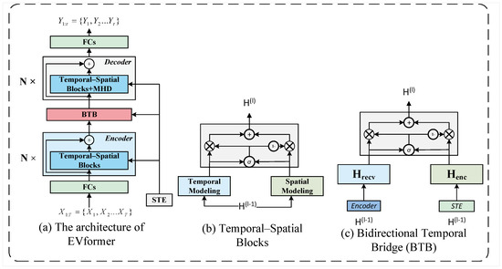
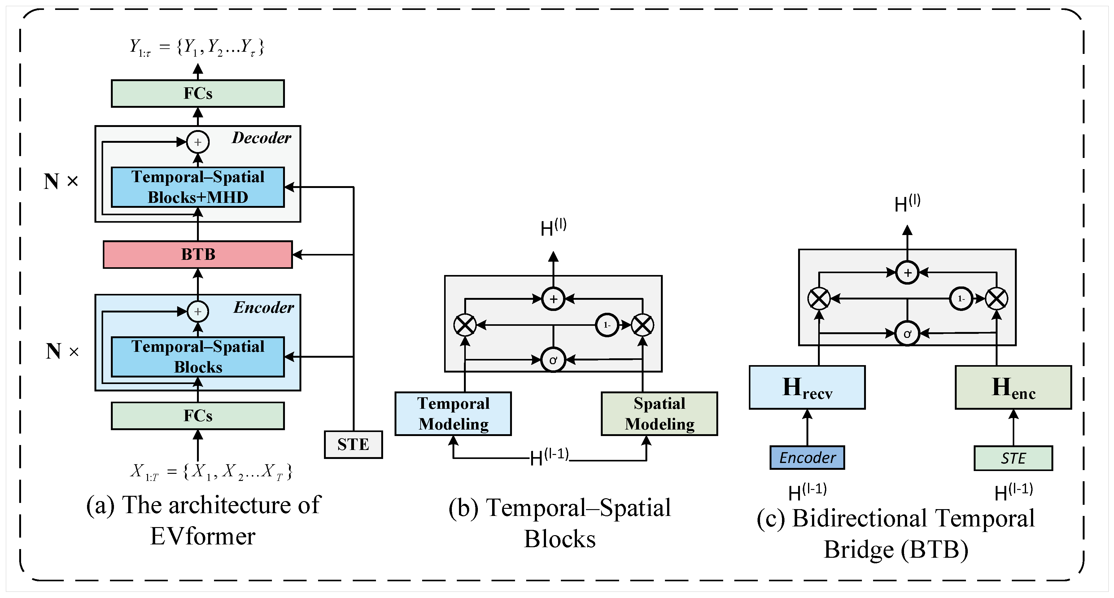
As illustrated in Figure 1, the proposed framework is a modularized spatio-temporal prediction model designed for urban electric vehicle (EV) charging demand forecasting. The model follows an encoder-decoder architecture, which is decoupled into multiple functional modules to effectively capture temporal evolution and spatial dependencies across city regions.

Figure 1. Overall architecture of the modular spatio-temporal prediction framework.

The overall pipeline consists of the following components:

• A Spatio-Temporal Embedding (STE) module that integrates spatial topology and temporal information into unified feature representations, providing the encoder with spatio-temporal priors.
• A stack of Temporal-Spatial Modeling blocks within the encoder and decoder to jointly learn temporal dependencies and spatial correlations.
• A Bidirectional Temporal Bridge (BTB) that dynamically transfers contextual information between historical and future representations.
• A Gated Fusion Unit embedded in each modeling block to adaptively balance spatial and temporal contributions.

In the encoding stage, historical observations are first embedded into a unified latent space and processed through multiple temporal-spatial blocks to learn high-level representations of charging dynamics. In the decoding stage, the model reconstructs multi-step future demand sequences based on the contextual information from the encoder. The BTB module connects the two stages, aligning temporal contexts across past and future horizons to ensure stable multi-step forecasting. This modular and hierarchical design allows the model to flexibly handle large-scale EV datasets, enhancing both predictive accuracy and computational efficiency.

3.3. Spatio-Temporal Embedding (STE)

To effectively capture the spatial structures and temporal regularities of EV charging demand, a Spatio-Temporal Embedding (STE) module is designed to integrate temporal periodicity and spatial topology into unified feature representations, providing the model with spatio-temporal priors.

Temporal Embedding: EV charging demand exhibits strong periodic patterns. Each time step t is represented by a learnable temporal embedding vector ${\mathrm{TE}}_t\in {\mathbb{R}}^D$, which combines sinusoidal encodings and trainable parameters:

$${\mathrm{TE}}_t=[sin\left({\omega }_t\right),cos\left({\omega }_t\right)]+e_t,$$

(9)

where ${\omega }_t$ is the normalized temporal index, and $e_t$ is a learnable embedding. This design enables the model to jointly capture explicit periodic cycles and implicit temporal dependencies.

Spatial Embedding: Each region node $v_i$ is assigned a trainable spatial embedding vector ${\mathrm{SE}}_i\in {\mathbb{R}}^D$:

$$\mathrm{SE}={[{\mathrm{SE}}_1,{\mathrm{SE}}_2,\dots ,{\mathrm{SE}}_N]}^{\top }\in {\mathbb{R}}^{N\times D},$$

(10)

where N denotes the number of regions. The spatial embedding provides structural and semantic priors, including location, charging density, and regional functionality.

Feature Fusion: At each time step t, the raw feature matrix $X_t\in {\mathbb{R}}^{N\times D}$ is fused with ${\mathrm{TE}}_t$ and SE as

$$H_t=\mathrm{MLP}\left([X_t;{\mathrm{TE}}_t;\mathrm{SE}]\right),$$

(11)

and all time steps are stacked to form the embedded sequence:

$$H_{1:T}=[H_1,H_2,\dots ,H_T]\in {\mathbb{R}}^{T\times N\times D}.$$

(12)

This embedding process provides the model with temporal periodicity and spatial awareness, serving as the foundation for downstream spatio-temporal modeling.

3.4. Temporal–Spatial Modeling

As illustrated in Figure 1b, the proposed model adopts a modular Temporal-Spatial Modeling block as the core computational unit in both the encoder and decoder. Each block contains three key components: a temporal attention module, a spatial attention module, and a gated fusion layer. The input of the l-th block is denoted as $H^{(l-1)}\in {\mathbb{R}}^{T\times N\times C}$, where $h_{i,t}^{(l-1)}$ represents the hidden state of region $v_i$ at time step t.

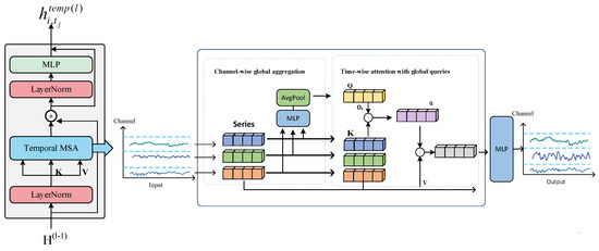
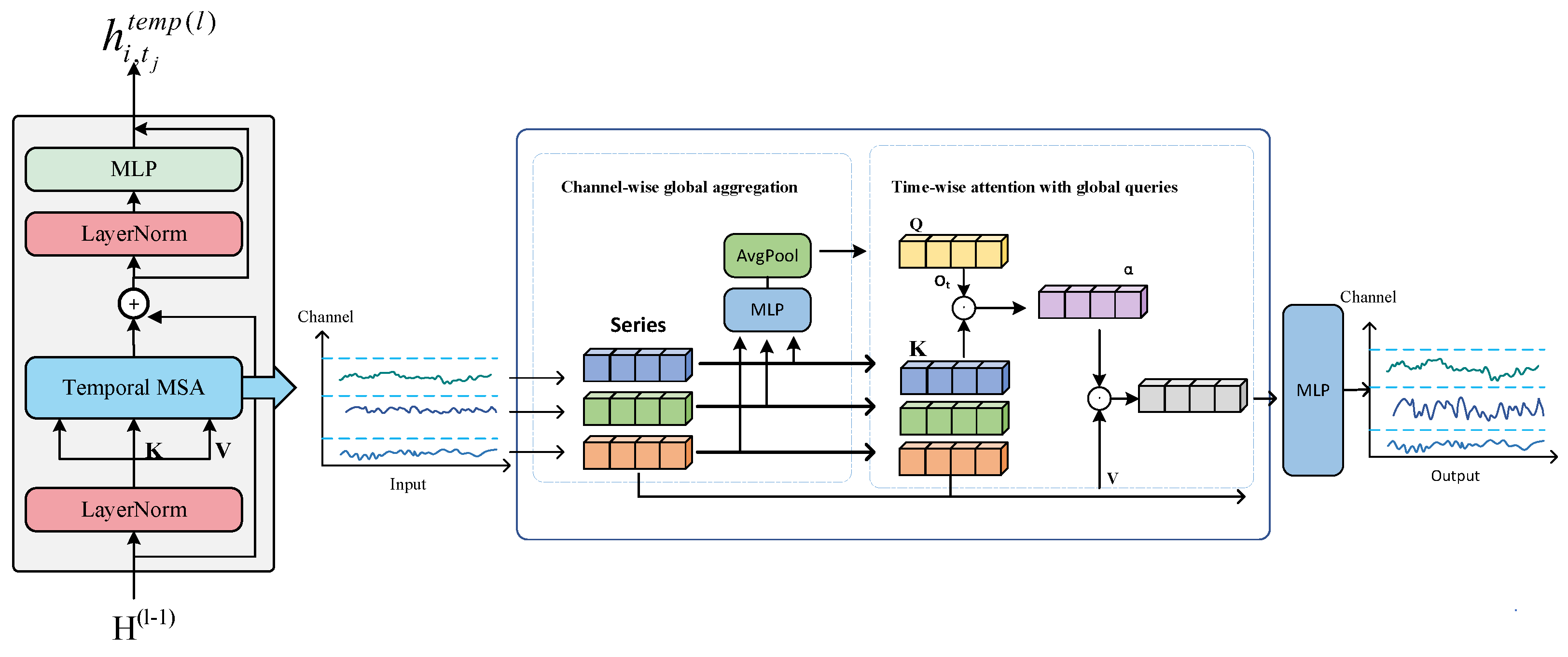
Temporal Attention: As shown in Figure 2, to jointly capture inter-variable interactions and temporal dependencies with reduced computational complexity, we adopt a two-stage channel-first temporal modeling strategy.

Figure 2. Architecture of the temporal modeling module.

Stage 1: Channel-wise global aggregation.Given the input to the l-th block $H^{(l-1)}\in {\mathbb{R}}^{T\times N\times C}$, we operate per node $v_i$ on its multi-variable sequence $S_i=H_{:,i,:}^{(l-1)}\in {\mathbb{R}}^{T\times C}$, where C denotes the number of variables (channels). At each time step t, we aggregate across channels to obtain a global context vector that summarizes cross-variable correlations:

$$o_t^{\left(i\right)}=\mathrm{Pool}\left(S_i[t,:]\right)\in {\mathbb{R}}^{d_g},O^{\left(i\right)}=[o_1^{\left(i\right)},\dots ,o_T^{\left(i\right)}]\in {\mathbb{R}}^{T\times d_g},$$

(13)

where $\mathrm{Pool}(·)$ denotes an average pooling or a lightweight MLP-plus-mean-pooling operation, and $d_g$ is the global context dimension. This step captures inter-variable (inter-channel) interactions at each time step, generating a unified global sequence representation.

Stage 2: Time-wise attention with channel-aware global queries. To model temporal dependencies, the global context $O^{\left(i\right)}$ is used as the query, while the original per-time channel vectors serve as the key and value. Unlike traditional self-attention mechanisms that require calculating pairwise attention between all time steps, our approach first aggregates inter-variable information into a global context, which significantly reduces the computational complexity. Traditional attention mechanisms suffer from quadratic time complexity of $O\left(T^{2}C\right)$, where T is the sequence length and C is the number of channels. By aggregating variables across time steps into a time-aligned channel-aware global query and then applies attention in a guided manner, avoiding direct time–time self-attention. This design reduces the complexity, making the model more efficient, especially for long-range temporal forecasting. For region $v_i$ and a target time step $t_j$, we compute

$$q_{t_j}^{\left(i\right)}=W_q{o}_{t_j}^{\left(i\right)},k_t^{\left(i\right)}=W_k{S}_i[t,:],v_t^{\left(i\right)}=W_v{S}_i[t,:],$$

(14)

where $q_{t_j}^{\left(i\right)},k_t^{\left(i\right)},v_t^{\left(i\right)}\in {\mathbb{R}}^d$ after projection. Causal multi-head attention is then applied over the past time steps

$$u_{t_j,t}^{\left(k\right)}={\displaystyle \frac{⟨f_1^{\left(k\right)}\left(q_{t_j}^{\left(i\right)}\right),f_2^{\left(k\right)}\left(k_t^{\left(i\right)}\right)⟩}{\sqrt{d}}},{\alpha }_{t_j,t}^{\left(k\right)}={\displaystyle \frac{exp\left(u_{t_j,t}^{\left(k\right)}\right)}{{\sum }_{t_r\in {\mathcal{N}}_{t_j}}exp\left(u_{t_j,t_r}^{\left(k\right)}\right)}},$$

(15)

and the updated temporal representation is obtained as

$$h_{i,t_j}^{\mathrm{temp}\left(l\right)}=\underset{k=1}{\overset{K}{⨁}}\left(\sum _{t\in {\mathcal{N}}_{t_j}}{\alpha }_{t_j,t}^{\left(k\right)}{f}_3^{\left(k\right)}\left(v_t^{\left(i\right)}\right),\right)$$

(16)

where $W_q$, $W_k$, and $W_v$ are learnable projection matrices, $f_1^{\left(k\right)}$, $f_2^{\left(k\right)}$, and $f_3^{\left(k\right)}$ are head-specific transformations, d is the head dimension, and K is the number of attention heads. A causal mask (and optionally a sliding window) is applied to maintain temporal order and prevent information leakage from the future.

This two-stage design first compresses multi-variable correlations into a global context $O^{\left(i\right)}$ and then re-weights historical time steps via attention guided by $O^{\left(i\right)}$. Compared with full pairwise temporal attention, this approach avoids the $O\left(T^{2}C\right)$ cross-time and cross-channel coupling, effectively reducing computational complexity while explicitly modeling both inter-variable relationships and temporal dependencies. Traditional attention mechanisms focus mainly on temporal dependencies and suffer from high computational overhead when processing long sequences. Our method, by reducing the computational cost and capturing inter-variable relationships before temporal attention is applied, enables better scalability and efficiency in long-sequence forecasting, which is crucial for large-scale real-time applications.

This step captures inter-variable (inter-channel) interactions at each time step, generating a unified global sequence representation. By aggregating variables before attention computation, our model improves feature extraction and interaction modeling, significantly enhancing both prediction accuracy and computational efficiency compared to traditional attention mechanisms that require pairwise calculations for each time step. This results in a more efficient model, especially suitable for large-scale, long-horizon time-series forecasting.

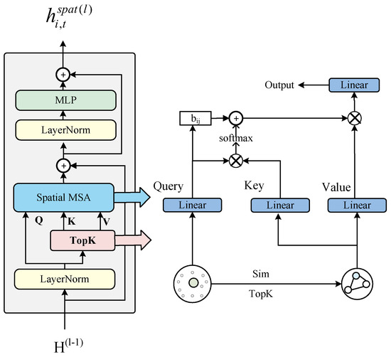
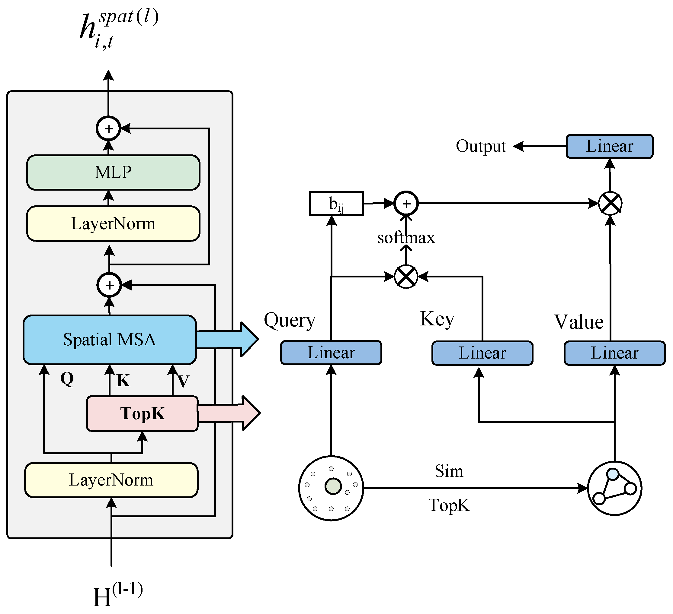
Spatial Attention: As shown in Figure 3, to accurately capture spatial correlations and heterogeneous interactions among city regions, we design a semantics-aware Top-K spatial attention mechanism.

Figure 3. The architecture of the proposed spatial attention mechanism.

Unlike conventional graph-based methods that rely on static adjacency, this module integrates both structural connectivity and regional semantics to adaptively refine spatial dependencies. Adjacency-based structural constraint. We first construct a physical adjacency matrix $\mathbf{A}\in {\mathbb{R}}^{N\times N}$ based on the urban topology, where $A_{ij}=1$ if regions $v_i$ and $v_j$ are geographically connected, and $A_{ij}=0$ otherwise. This constraint ensures that each node only attends to physically meaningful neighbors and reduces redundant computations.

Semantic embedding and similarity filtering. Each region $v_i$ is assigned a semantic embedding vector $s_i\in {\mathbb{R}}^{d_s}$, representing static urban attributes such as land-use type, charging policy, and charger density. The semantic similarity between two regions is computed as

$$\mathrm{sim}(i,j)=cos(s_i,s_j)={\displaystyle \frac{s_i^{\top }{s}_j}{\parallel s_i\parallel \parallel s_j\parallel }}.$$

(17)

For each node $v_i$, we retain the Top-K most semantically similar neighbors within its structural neighborhood ${\mathcal{N}}_i^A=\{v_j\mid A_{ij}=1\}$:

$${\mathcal{N}}_i^{\mathrm{top}}=\mathrm{TopK}\left(\mathrm{sim}(i,j)\right),j\in {\mathcal{N}}_i^A.$$

(18)

This hybrid selection strategy filters out semantically irrelevant nodes while preserving structural connectivity.

Attention computation: For each node $v_i$ at time step t, the spatial dependency between $v_i$ and its Top-K neighbors $v_j\in {\mathcal{N}}_i^{\mathrm{top}}$ is computed using multi-head attention:

$${\alpha }_{ij}^{\left(k\right)}={\displaystyle \frac{exp\left(q_i{W}_q^{\left(k\right)}\right){\left(k_j{W}_k^{\left(k\right)}\right)}^{\top }+b_{ij}}{{\sum }_{m\in {\mathcal{N}}_i^{\mathrm{top}}}exp\left(q_i{W}_q^{\left(k\right)}\right){\left(k_m{W}_k^{\left(k\right)}\right)}^{\top }+b_{im}}},$$

(19)

$$h_{i,t}^{\mathrm{spat}\left(l\right)}=\underset{k=1}{\overset{K}{⨁}}\left(\sum _{j\in {\mathcal{N}}_i^{\mathrm{top}}}{\alpha }_{ij}^{\left(k\right)}{W}_v^{\left(k\right)}{h}_{j,t}^{(l-1)}\right),$$

(20)

where $q_i$, $k_j$, and $v_j$ represent query, key, and value vectors of nodes $v_i$ and $v_j$, respectively; $b_{ij}$ is a learnable bias derived from the semantic distance between regions. The bias term allows the model to account for functional or pricing differences between regions that are not purely spatial.

This semantics-aware attention enables the model to simultaneously capture fine-grained local dependencies and coarse-grained functional correlations across distant regions. By restricting attention to the Top-K semantically relevant neighbors, the complexity of spatial modeling is reduced from $O\left(N^2\right)$ to $O\left(K^2\right)$ while preserving key structural and semantic relationships.

As shown in Figure 1b, to adaptively balance the contributions of temporal and spatial dependencies, a Gated Fusion Unit is employed to integrate the outputs of the temporal and spatial attention modules within each block. This design allows the model to dynamically determine which dimension (temporal or spatial) should dominate under varying charging demand patterns.

Given the outputs of the temporal and spatial attention modules at the l-th block, denoted as $H_{\mathrm{temp}}^{\left(l\right)}$ and $H_{\mathrm{spat}}^{\left(l\right)}$, respectively, both of shape ${\mathbb{R}}^{T\times N\times C}$, the fused representation is obtained as

$$H^{\left(l\right)}=z\odot H_{\mathrm{spat}}^{\left(l\right)}+(1-z)\odot H_{\mathrm{temp}}^{\left(l\right)},$$

(21)

where ⊙ denotes element-wise multiplication, and $z\in [0,1]$ is a gating coefficient computed as

$$z=\sigma \left(H_{\mathrm{spat}}^{\left(l\right)}{W}_{z,1}+H_{\mathrm{temp}}^{\left(l\right)}{W}_{z,2}+b_z\right),$$

(22)

with $W_{z,1},W_{z,2}\in {\mathbb{R}}^{C\times C}$, and $b_z\in {\mathbb{R}}^C$ being learnable parameters and $\sigma (·)$ representing the sigmoid activation.

This adaptive gating mechanism dynamically regulates the flow of information from temporal and spatial pathways, enabling the model to focus on either short-term temporal fluctuations or spatial correlations when necessary. By learning gate values for each node and time step, the module effectively enhances feature fusion and stabilizes optimization across multiple scales of spatio-temporal dependencies.

3.5. Bidirectional Temporal Bridge and Multi-Horizon Decoder

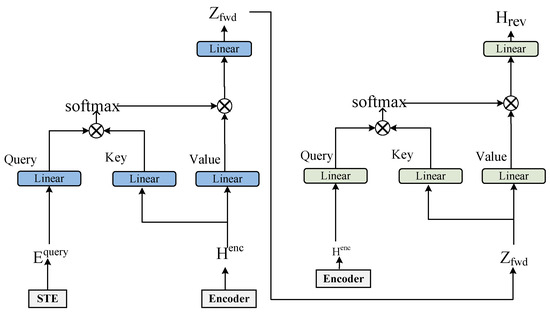
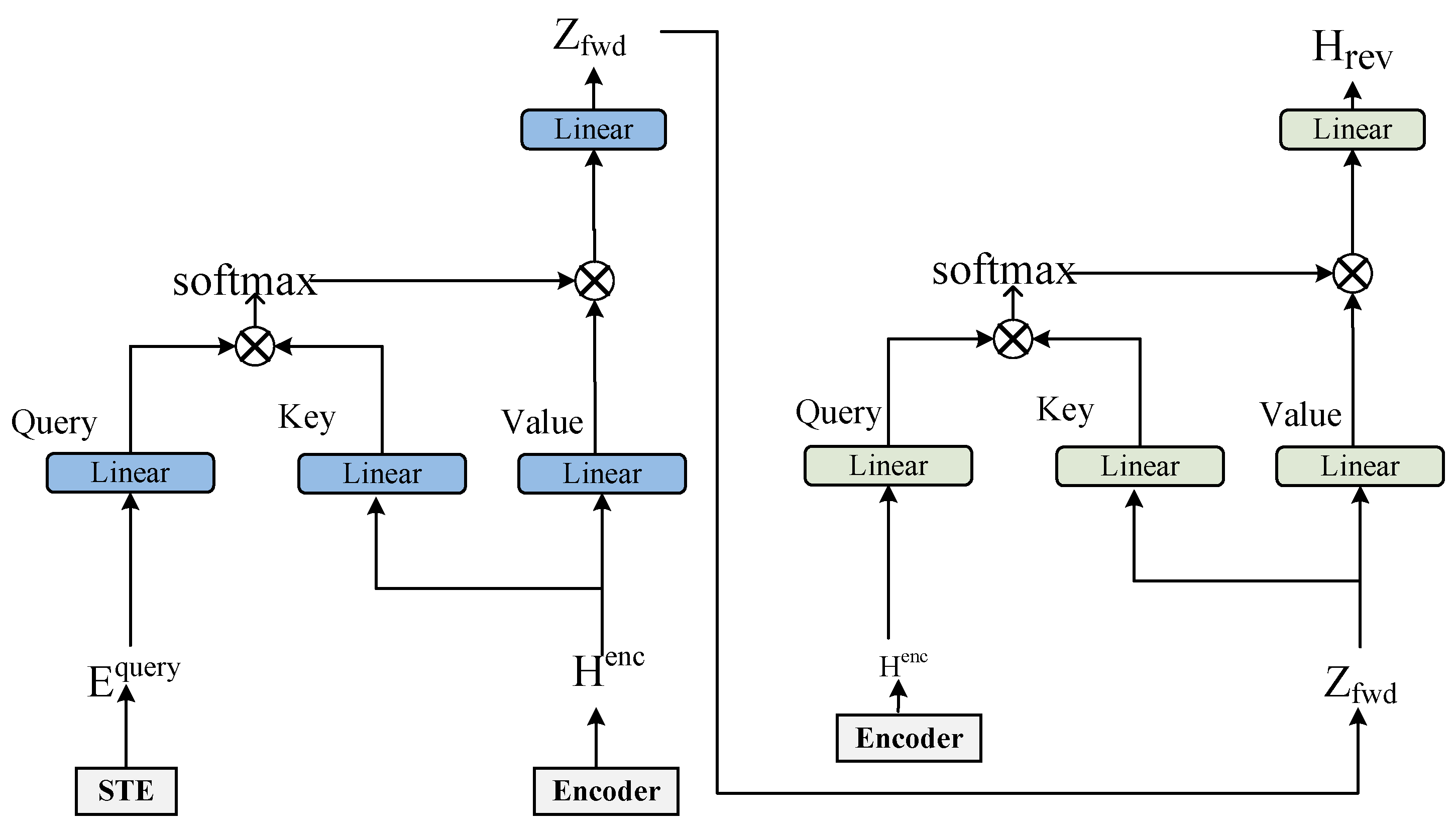
To ensure efficient information transfer between the encoder and decoder while enhancing multi-step prediction stability, we introduce a Bidirectional Temporal Bridge (BTB) and a Multi-Horizon Decoder (MHD). As illustrated in Figure 4, the BTB serves as a dynamic connector that aligns temporal contexts between historical and future representations, while the MHD is designed to predict charging demand across multiple temporal horizons simultaneously.

Figure 4. Overall architecture of the proposed bidirectional temporal bridge.

In conventional transfor based forecasting frameworks, the encoder-to-decoder mapping is unidirectional, which often leads to information loss between the historical and future temporal domains. To alleviate this, BTB introduces a dual-path attention mechanism that allows bidirectional interaction.

Specifically, given the encoder output $H^{\mathrm{enc}}\in {\mathbb{R}}^{T\times N\times C}$ and the temporal embeddings of future prediction steps $E^{\mathrm{query}}\in {\mathbb{R}}^{\tau \times C}$, we first compute a forward attention mapping from the historical states to the prediction context:

$$Z_{\mathrm{fwd}}=\mathrm{MultiHeadAttn}\left(E^{\mathrm{query}},H^{\mathrm{enc}},H^{\mathrm{enc}}\right)\in {\mathbb{R}}^{\tau \times N\times C},$$

(23)

then, a reverse refinement is performed by allowing the encoder to re-attend to the generated predictive context:

$$H_{\mathrm{rev}}=\mathrm{MultiHeadAttn}\left(H^{\mathrm{enc}},Z_{\mathrm{fwd}},Z_{\mathrm{fwd}}\right),$$

(24)

finally, a gating function adaptively fuses the two directions:

$$H_{\mathrm{bridge}}=\lambda H_{\mathrm{rev}}+(1-\lambda )H^{\mathrm{enc}},\lambda =\sigma \left(W[H^{\mathrm{enc}};Z_{\mathrm{fwd}}]+b\right).$$

(25)

This bidirectional bridge establishes a feedback loop between the past and future temporal domains, enabling dynamic contextual alignment and mitigating cumulative forecasting drift across time steps.

Multi-Horizon Decoder (MHD). On top of $H_{\mathrm{bridge}}$, the decoder generates multi-step charging demand predictions. Unlike conventional single-scale decoders, the MHD adopts a hierarchical design to model temporal dependencies at different forecasting horizons. Specifically, the prediction horizon $\tau$ is divided into three granular ranges: short term, mid-term, and long-term, each modeled by an independent decoder layer:

$$Y^{\left(k\right)}={\mathrm{Decoder}}_k\left(H_{\mathrm{bridge}}\right),k\in \{1,2,3\},$$

(26)

the final prediction is obtained through adaptive fusion:

$$\widehat{Y}=\sum _{k=1}^3{\alpha }_k{Y}^{\left(k\right)},\sum _{k=1}^3{\alpha }_k=1,$$

(27)

where ${\alpha }_k$ denotes learnable fusion coefficients. This design allows the decoder to emphasize different temporal patterns at distinct horizons, improving stability and accuracy for both short-term fluctuations and long-term demand evolution.

3.6. Gated Fusion and Training Objective

To generate the final prediction, the outputs of the temporal–spatial modeling blocks are adaptively fused and optimized through a unified training objective. The gating mechanism dynamically adjusts the contributions of temporal and spatial dependencies across different layers and time steps, enabling robust multi-horizon forecasting.

Global Gated Fusion. After obtaining the temporal and spatial representations from each block, the model aggregates them via a global gating mechanism to produce the final latent feature representation $H^{\left(l\right)}$:

$$H^{\left(l\right)}=z\odot H_{\mathrm{spat}}^{\left(l\right)}+(1-z)\odot H_{\mathrm{temp}}^{\left(l\right)},$$

(28)

where ⊙ denotes element-wise multiplication, and z is the adaptive gating coefficient:

$$z=\sigma (W_z[H_{\mathrm{spat}}^{\left(l\right)};H_{\mathrm{temp}}^{\left(l\right)}]+b_z),$$

(29)

with $W_z$ and $b_z$ as learnable parameters. This adaptive fusion enables the network to focus on either short-term temporal patterns or spatial dependencies as needed, leading to a more balanced spatio-temporal representation.

Prediction Mapping. The fused representation $H^{\left(L\right)}$ is projected into the prediction space using a fully connected mapping layer:

$${\widehat{Y}}_{1:\tau }=\mathrm{MLP}\left(H^{\left(L\right)}\right),$$

(30)

where ${\widehat{Y}}_{1:\tau }\in {\mathbb{R}}^{\tau \times N\times D^{\prime }}$ denotes the predicted charging demand over $\tau$ future time steps, and $D^{\prime }$ represents the target feature dimension (e.g., charging power or duration), L denotes the last time step modeling block.

Training Objective. The model is trained in a supervised manner by minimizing the mean absolute error (MAE) between predicted and ground-truth values:

$$\mathcal{L}={\displaystyle \frac{1}{\tau N}}\sum _{t=1}^{\tau }\sum _{i=1}^N\left|{\widehat{Y}}_{t,i}-Y_{t,i}\right|.$$

(31)

This objective encourages accurate point-wise forecasting while maintaining robustness to outliers in high-variance urban charging demand data.

To ensure stability, the entire framework—comprising the encoder, BTB, decoder, and gated fusion—is trained end-to-end using back-propagation. Such unified optimization allows each module to cooperatively learn temporal dynamics, spatial dependencies, and inter-horizon consistency, achieving high forecasting precision with efficient computation.

4. Experimental Results and Discussion

4.1. Dataset

The dataset used in this study is obtained from a publicly available mobile application dataset, namely, ST-EVCDP, which provides real-time availability information of public charging piles. The data were collected in Shenzhen, China, from 19 June to 18 July 2022, covering a total of 18,061 public charging piles with a minimum sampling interval of 5 min. The dataset is publicly available at https://github.com/IntelligentSystemsLab/ST-EVCDP (accessed on 20 January 2025).

In the spatial dimension, the city is partitioned into 247 regional nodes, and a spatial graph with 1006 edges is constructed based on centroid distances between regions. Each node contains multiple features, including charging demand, charging duration, pile utilization rate, pricing mechanism (fixed/dynamic), regional functional type (residential, commercial, and industrial), and charging pile density.

Prior to training, the dataset is preprocessed with the following steps:

(i) Data partitioning: The data are divided into training, validation, and test sets in chronological order with a ratio of 7:1:2.

(ii) Missing value handling: Missing entries, if present, are handled using a combination of linear interpolation and forward filling. In the dataset used in this study, no missing values were observed; therefore, this preprocessing step was not triggered in practice.

(iii) Normalization: Continuous features are standardized using Z-score normalization:

$$\overline{x}={\displaystyle \frac{x-\mu }{\sigma }}.$$

(32)

4.2. Model Settings

The proposed model is implemented using the PyTorch framework (version 2.60) and trained on an NVIDIA RTX 4090 GPU with 48GB of memory, utilizing CUDA 12.4. The proposed model is implemented using the PyTorch framework. We employ the Adam optimizer with an initial learning rate of 0.001, which is gradually decayed using a cosine annealing scheduler. The batch size is set to 64, and the model is trained for up to 80 epochs. Early stopping is applied if the validation loss does not improve for 10 consecutive epochs.

The historical window length is set to $T=12$ (i.e., the past 1 h with a 5 min sampling interval). The prediction horizons are $\tau =3,6,9$, corresponding to 15, 30, and 45 min, respectively. The hidden dimension is set to $d=64$, and each temporal and spatial attention mechanism uses eight attention heads. In the spatial modeling module, the Top-K parameter for neighbor selection is set to $K=20$, meaning that each node attends only to its 20 most semantically relevant neighbors. This value is determined through hyperparameter tuning on the validation set and remains fixed for all experiments. Both the encoder and decoder consist of $N=3$ stacked spatio-temporal modeling layers, where each layer comprises a temporal sub-module and a spatial sub-module. These two components are integrated via a gating mechanism to jointly model temporal and spatial dependencies. The model is optimized using the Mean Absolute Error (MAE) loss, which improves robustness against outliers. For performance evaluation, three commonly used metrics are adopted: Mean Absolute Error (MAE), Root Mean Squared Error (RMSE), and Mean Absolute Percentage Error (MAPE). These metrics, respectively, measure absolute deviation, squared deviation, and relative error, providing a comprehensive evaluation of the forecasting accuracy and stability. The model showed smooth convergence during the 80 epochs, with no significant overfitting observed. The consistent performance on both the training and validation sets further confirms the model’s stability.

4.3. Baselines for Comparison

To comprehensively evaluate the effectiveness of the proposed model, we compare it with a wide range of representative baselines from four categories:

Traditional statistical methods:

• VAR [18]: Vector Autoregression, a widely used linear multivariate forecasting model.
• Lasso [19]: Linear regression with L1 regularization for sparse feature selection.
• KNN: K-Nearest Neighbor regression, which predicts future demand based on similar historical patterns.

Deep learning methods:

• FCNN [20]: A fully connected neural network baseline without explicit temporal modeling.
• RNN/LSTM [4]: Recurrent architectures designed to capture temporal dependencies.

Graph-based spatio-temporal models:

• GCN [21]: Graph Convolutional Network that models spatial correlations using static adjacency.
• STGCN [15]: A convolutional model that couples temporal CNNs with graph convolutions.
• DCRNN [16]: A diffusion-convolution-based recurrent model capturing dynamic spatial propagation.
• MTGNN [22]: A multivariate time-series graph neural network that jointly models spatial dependencies via graph convolution and temporal dependencies via temporal convolution and gating mechanisms.
• GraphWaveNet [23]: A graph-based forecasting model that integrates graph convolution with WaveNet-style dilated temporal convolutions to capture long-range temporal dependencies.

Attention-based spatio-temporal methods:

• GAT [24]: Graph Attention Network that learns attention weights between connected nodes.
• AST-GAT [25]: A dynamic attention-based model for adaptive spatio-temporal dependency learning.
• PAG [26]: A physics-aware attention model integrating structural priors into the learning process.

4.4. Model Comparison

Table 1 compares the performance of the EVformer model with various baseline models across three forecasting horizons: 15 min, 30 min, and 45 min, using RMSE, MAE, and MAPE.

Table 1. Comparison of different models on EV charging demand prediction across multiple horizons (15 min, 30 min, and 45 min).

Metric (${10}^{-2}$)	RMSE			MAE			MAPE
Model	15 min	30 min	45 min	15 min	30 min	45 min	15 min	30 min	45 min
VAR	5.55	8.51	11.25	8.11	10.04	10.98	53.57	64.02	65.93
Lasso	4.33	6.32	7.98	2.51	3.75	4.66	12.28	19.43	25.64
KNN	4.58	6.48	7.94	2.49	3.68	4.53	11.56	16.60	20.79
FCNN	3.37	5.75	7.45	1.92	3.26	4.31	9.74	15.86	22.37
LSTM	3.59	6.64	7.50	1.88	3.25	4.75	8.91	14.91	21.01
GCN	4.41	6.65	8.10	6.30	7.34	8.06	40.26	46.17	49.40
GAT	3.62	5.78	7.44	2.06	3.34	4.35	10.26	16.77	23.65
STGCN	3.58	5.57	6.88	4.93	5.65	6.60	31.42	32.59	43.05
DCRNN	3.75	5.41	6.75	2.25	3.35	4.23	11.32	16.08	19.94
MTGNN	3.54	5.39	6.60	2.21	3.32	4.11	11.15	16.02	18.77
GraphWaveNet	3.49	5.41	6.67	2.18	3.33	4.17	10.86	15.95	19.21
AST-GAT	3.44	5.38	6.57	2.05	3.38	3.96	9.94	18.04	17.83
PAG	3.15	5.15	6.52	1.88	3.15	3.94	9.34	14.57	17.55
EVformer	3.06	4.98	6.45	1.78	3.05	3.93	8.90	12.49	17.49

Traditional models like VAR, Lasso, and KNN perform well for short-term forecasting but deteriorate as the prediction horizon increases. For instance, VAR’s RMSE increases from 5.55 (15 min) to 11.25 (45 min), and its MAPE rises from 53.57% to 65.93%, indicating significant performance degradation. Deep learning models, including FCNN and LSTM, show improvements in short-term forecasts, with FCNN achieving an RMSE of 3.37 at 15 min. However, they struggle in long-term forecasting due to a lack of spatial dependency modeling, with LSTM’s MAE rising from 1.88 (15 min) to 4.75 (45 min). Graph-based models like GCN, STGCN, and DCRNN perform better in capturing spatial dependencies. STGCN achieves an RMSE of 5.57 at the 30 min horizon but is limited by its static adjacency matrix, resulting in decreased performance for longer horizons.MTGNN and GraphWaveNet achieve competitive performance among graph-based spatio-temporal forecasting models. MTGNN benefits from its graph-based spatial modeling and temporal convolution design, while GraphWaveNet effectively captures long-range temporal dependencies through dilated convolutions. However, both models rely on relatively coupled spatio-temporal representations, which may limit their ability to flexibly adapt to dynamic temporal patterns. In contrast, EVformer consistently outperforms these baselines by explicitly decoupling temporal and spatial modeling, enabling more efficient temporal representation learning and adaptive spatial dependency modeling.

Attention-based models such as GAT, AST-GAT, and PAG further improve by modeling flexible spatio-temporal dependencies. PAG, with an RMSE of 5.15 and MAE of 3.15 at 15 min, performs better than previous models but still falls short of EVformer’s performance. EVformer outperforms all baselines across all metrics and time horizons. At the 30 min horizon, EVformer achieves the lowest RMSE (4.98), MAE (3.05), and MAPE (12.49%), outperforming the best baseline (PAG) by 3.8%, 2.1%, and 3.1%, respectively. The advantage becomes even more significant at the 45 min horizon, where EVformer achieves an RMSE of 6.45, MAE of 3.93, and MAPE of 17.49%, demonstrating its strong ability to model long-range dependencies.

EVformer maintains high accuracy even in long-term forecasting. This is largely due to the introduction of our global-aware temporal modeling strategy, which aggregates variables and reduces computational complexity. As a result, EVformer can efficiently handle long sequences while maintaining strong performance, unlike traditional methods that face significant computational overhead and limited ability to model inter-variable relationships. In addition to its high accuracy, EVformer provides strong interpretability through its dynamic spatial attention mechanism. This mechanism enables the model to highlight which neighboring stations have the most influence on predictions, offering transparency in how the model makes decisions. In conclusion, EVformer consistently delivers superior performance and is well suited for large-scale, real-world EV charging demand forecasting applications.

4.5. Ablation Study

To assess the impact of each module in the proposed model, we conducted a series of ablation experiments on the 30 min forecasting task ($\tau =3,6,9$). The results of the ablation study are summarized in Table 2, where we evaluate the contribution of each module—temporal modeling, spatial attention, bidirectional temporal bridge (BTB), and gated fusion—to the overall performance.

Table 2. Results of ablation experiment for EVformer.

Interval	Model	RMSE	MAPE
15 min	EVformer (Full)	3.06	8.90
	w/o Temporal	3.32	10.42
	w/o Spatial	3.28	10.15
	w/o BTB	3.18	9.55
	w/o Gating	3.14	9.38
30 min	EVformer (Full)	4.98	12.49
	w/o Temporal	5.42	14.02
	w/o Spatial	5.46	14.31
	w/o BTB	5.16	13.21
	w/o Gating	5.28	12.98
45 min	EVformer (Full)	6.45	17.49
	w/o Temporal	7.01	19.82
	w/o Spatial	6.96	19.55
	w/o BTB	6.72	18.63
	w/o Gating	6.60	18.15

Impact of Temporal Modeling: To assess the contribution of the temporal modeling module, we evaluate the following variants: (a) w/o Temporal: The model without temporal modeling, where temporal dependencies are ignored. (b) Average Pooling: Temporal modeling is replaced with average pooling, which aggregates past information uniformly. The results are shown in Table 2. First, we observe that removing the temporal modeling module leads to a significant increase in RMSE and MAPE, particularly at the 45 min prediction horizon. This confirms the importance of temporal modeling in capturing long-term dependencies and handling dynamic variations in charging demand.

Impact of Spatial Modeling: In this experiment, we replace the dynamic Top-K spatial attention mechanism with a static Graph Convolutional Network (GCN) to evaluate the contribution of spatial modeling. The variant w/o Spatial lacks dynamic spatial attention and relies on fixed adjacency relationships. The results show that this change leads to a notable increase in both RMSE and MAPE across all time horizons. At 15 min, RMSE increases by 7.2% and MAPE rises by 13.9%. These findings highlight the necessity of dynamic spatial attention for accurately capturing the dependencies between charging stations, especially as spatial interactions can vary significantly over time.

Impact of Bidirectional Temporal Bridge (BTB): The BTB module is designed to align the temporal context between historical and future representations. To study its effect, we remove the BTB module, resulting in the w/o BTB variant. The ablation results demonstrate a smaller yet noticeable decline in performance, with RMSE increasing by 3.9% and MAPE rising by 7.3% at 15 min. This suggests that the BTB module plays a crucial role in enhancing the stability and accuracy of multi-step forecasting by refining the alignment of temporal contexts across time steps.

Impact of Gated Fusion: In this experiment, we replace the gated fusion mechanism with simple concatenation of spatial and temporal features. The w/o Gating variant shows a smaller increase in RMSE (2.6%) and MAPE (5.4%) compared to the full model. Although the effect of the gating mechanism is less pronounced than the other modules, its removal still leads to a performance drop. This highlights the importance of adaptively balancing spatial and temporal features, particularly when their influence varies across different time periods and regions.

4.6. Parameter Sensitivity Analysis

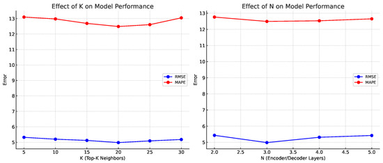
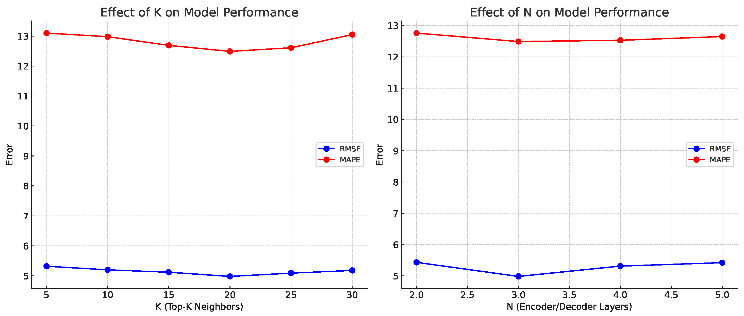
To assess the robustness of the proposed model under different hyperparameter settings, we conduct a parameter sensitivity analysis focusing on two key factors: the neighbor selection parameter K in the spatial module and the model depth N in the encoder–decoder architecture. The results are visualized in Figure 5, which illustrates the variations of MAPE and RMSE under different configurations.

Figure 5. Sensitivity analysis of hyperparameters. The figure reports the performance variations of the proposed model under different hyperparameter configurations: neighbor selection parameter $K\in \{5,10,15,20,20,30\}$; model depth $N\in \{2,3,4,5\}$. Results are evaluated by MAPE and RMSE on the Shenzhen EV charging dataset.

As illustrated in Figure 5, when K is too small (e.g., $K=5$), the model fails to capture sufficient spatial correlations, leading to noticeable errors. Increasing K to 20 yields the lowest MAPE and RMSE by effectively balancing local structural dependencies and long-range semantic relevance. However, further increasing K to 30 introduces redundant neighbors, weakening attention allocation and degrading performance. These findings indicate that an appropriate neighborhood size is crucial for maintaining both efficiency and predictive accuracy.

We further examine the impact of varying the number of stacked temporal–spatial blocks in both the encoder and decoder: $N\in \{2,3,4,5\}$. As shown in Figure 5, a shallow architecture ($N=2$) lacks sufficient representation capacity, particularly for long-horizon forecasting. Increasing the depth to $N=3$ significantly improves accuracy, while $N=4$ brings only marginal gains. When N is increased to 5, the error begins to rise and computational overhead grows substantially, likely due to overfitting and increased optimization difficulty.

The parameter sensitivity analysis demonstrates that both the neighbor selection parameter K and the model depth N have a substantial impact on overall performance. For the Shenzhen EV charging demand dataset, the optimal configuration is

$$K=20,N=3,$$

(33)

which provides the best trade-off between computational cost and forecasting accuracy.

4.7. Computational Efficiency and Complexity Analysis

In addition to predictive accuracy, computational efficiency is also a critical metric for evaluating spatio-temporal forecasting models. We analyze the proposed method from both the perspectives of theoretical complexity and practical runtime efficiency.

In the temporal modeling component, conventional Transformer-based approaches require global attention computations across all time steps, resulting in a complexity of $O\left(T^{2}d\right)$, where d denotes the feature dimension. This incurs substantial computational overhead in long-sequence forecasting. By contrast, our method aggregates channels to obtain global trend representations and introduces attention only during cross-channel interactions, thereby reducing computational overhead in practice. This significantly enhances scalability while maintaining strong modeling capability.

In the spatial modeling component, standard global attention mechanisms compute interactions among all nodes, leading to a complexity of $O\left(N^{2}d\right)$. In our design, a topology-constrained Top-K semantic filtering strategy restricts each node’s interactions to its K most relevant neighbors, reducing the complexity to $O\left(K^2\right)$. This approach effectively eliminates redundant computations in large-scale urban graphs. Here, K is typically much smaller than N, making $O\left(K^{2}d\right)$ significantly more efficient than $O\left(N^{2}d\right)$.

To evaluate computational efficiency in practical applications, we compared different models in terms of parameter size, training time, and inference time. The results are reported in Table 3. STGCN shows the highest efficiency due to its simple structure, but its predictive accuracy is limited. DCRNN and PAG exhibit higher computational costs, reflecting the overhead of recurrent structures and complex attention mechanisms. GMAN has the largest parameter size and computation cost, highlighting its scalability limitations. In contrast, our model achieves a lighter parameter scale while maintaining high predictive accuracy, and its training and inference speed outperform other attention-based models, only slightly slower than STGCN, demonstrating strong efficiency and practicality.

Table 3. Comparison of model efficiency in terms of parameter size, training time, and inference time.

Model	Params (M)	Train Time/Epoch (s)	Inference Time/Step (ms)
STGCN	2.3	35	4.2
DCRNN	3.8	52	6.1
GMAN	5.6	68	7.3
PAG	4.9	61	6.9
Ours	3.9	46	5.7

5. Conclusions

This paper addresses the challenges of complex spatio-temporal dependencies and high computational costs in urban electric vehicle charging demand forecasting. To this end, we propose a modular and decoupled spatio-temporal prediction framework. The core novelty of the proposed EVformer lies in its explicit decoupling of temporal and spatial modeling, where global trend-aware temporal modeling and adaptive graph-based spatial attention are jointly integrated through a gated fusion mechanism. This design enables efficient cross-channel temporal interaction and scalable spatial dependency learning without relying on fixed station identities. Experiments conducted on a real-world dataset consisting of 18,061 public charging piles in Shenzhen demonstrate that EVformer consistently outperforms representative spatio-temporal baselines. Quantitatively, EVformer achieves approximately 1–6% relative RMSE reduction compared with state-of-the-art graph-based models (e.g., STGCN, DCRNN, MTGNN, and GraphWaveNet) in long-horizon forecasting (45 min) and up to around 13% improvement in short-horizon prediction (15 min). Moreover, EVformer attains the lowest MAE and MAPE across all prediction horizons, confirming its superior accuracy and robustness.

From a practical perspective, further reducing the RMSE to the 1% level would require additional factors beyond architectural improvements, including longer-term and multi-season datasets, the incorporation of exogenous variables such as weather conditions and traffic flow, and finer-grained temporal resolution. In addition, since spatial dependencies are modeled through graph-based representations and adaptive attention rather than fixed charging pile identities, the proposed framework is inherently scalable to changes in charging infrastructure density, enabling effective adaptation to evolving urban charging networks.

Future work will mainly focus on two directions: first, incorporating external data sources (e.g., weather conditions and traffic flow) to further improve forecasting accuracy; second, developing more lightweight model structures to better meet the requirements of real-time scheduling and edge computing scenarios. Furthermore, extending the dataset to cover longer time spans and multiple seasons will enable a more comprehensive evaluation of seasonal effects and cross-seasonal generalization.

References

- Ghani, A.A.; Abdullah, N.; Saidur, R.; Pandey, A. Assessing technological-driven challenges and policies associated with electric vehicle (EV) adoption. Transp. Policy 2025, 169, 167–177. [Google Scholar] [CrossRef] [Scilit]
- Ullah, I.; Zheng, J.; Jamal, A.; Zahid, M.; Almoshageh, M.; Safdar, M. Electric vehicles charging infrastructure planning: A review. Int. J. Green Energy 2024, 21, 1710–1728. [Google Scholar] [CrossRef] [Scilit]
- Wang, F.Y.; Lin, Y.; Ioannou, P.A.; Vlacic, L.; Liu, X.; Eskandarian, A.; Lv, Y.; Na, X.; Cebon, D.; Ma, J. Transportation 5.0: The DAO to safe, secure, and sustainable intelligent transportation systems. IEEE Trans. Intell. Transp. Syst. 2023, 24, 10262–10278. [Google Scholar] [CrossRef] [Scilit]
- Graves, A. Long short-term memory. In Supervised Sequence Labelling with Recurrent Neural Networks; Springer: Berlin/Heidelberg, Germany, 2012; pp. 37–45. [Google Scholar]
- Kipf, T.N.; Welling, M. Semi-Supervised Classification with Graph Convolutional Networks. In Proceedings of the International Conference on Learning Representations, Toulon, France, 24–26 April 2017. [Google Scholar]
- Vaswani, A.; Shazeer, N.; Parmar, N.; Uszkoreit, J.; Jones, L.; Gomez, A.N.; Kaiser, Ł.; Polosukhin, I. Attention is all you need. Adv. Neural Inf. Process. Syst. 2017, 30, 5998–6008. [Google Scholar]
- Liang, X.; Yang, E.; Deng, C.; Yang, Y. CrossFormer: Cross-modal representation learning via heterogeneous graph transformer. ACM Trans. Multimed. Comput. Commun. Appl. 2024, 20, 1–21. [Google Scholar]
- Liu, Y.; Hu, T.; Zhang, H.; Wu, H.; Wang, S.; Ma, L.; Long, M. iTransformer: Inverted transformers are effective for time series forecasting. arXiv 2023, arXiv:2310.06625. [Google Scholar]
- Zhou, X.; Wang, J.; Wang, J.; Guan, Q. Predicting air quality using a multi-scale spatiotemporal graph attention network. Inf. Sci. 2024, 680, 121072. [Google Scholar] [CrossRef] [Scilit]
- Chauhan, J.; Raghuveer, A.; Saket, R.; Nandy, J.; Ravindran, B. Multi-variate time series forecasting on variable subsets. In Proceedings of the 28th ACM SIGKDD Conference on Knowledge Discovery and Data Mining, Edmonton, AB, Canada, 23–26 July 2022; pp. 76–86. [Google Scholar]
- Li, J.; Wang, S.; Zhang, J.; Miao, H.; Zhang, J.; Yu, P.S. Fine-grained urban flow inference with incomplete data. IEEE Trans. Knowl. Data Eng. 2022, 35, 5851–5864. [Google Scholar] [CrossRef] [Scilit]
- Patari, N.; Venkataramanan, V.; Srivastava, A.; Molzahn, D.K.; Li, N.; Annaswamy, A. Distributed optimization in distribution systems: Use cases, limitations, and research needs. IEEE Trans. Power Syst. 2021, 37, 3469–3481. [Google Scholar] [CrossRef] [Scilit]
- Zhou, H.; Zhang, S.; Peng, J.; Zhang, S.; Li, J.; Xiong, H.; Zhang, W. Informer: Beyond efficient transformer for long sequence time-series forecasting. In Proceedings of the AAAI Conference on Artificial Intelligence, Vancouver, BC, Canada, 2–9 February 2021; Volume 35, pp. 11106–11115. [Google Scholar]
- Wu, H.; Xu, J.; Wang, J.; Long, M. Autoformer: Decomposition transformers with auto-correlation for long-term series forecasting. Adv. Neural Inf. Process. Syst. 2021, 34, 22419–22430. [Google Scholar]
- Hedegaard, L.; Heidari, N.; Iosifidis, A. Continual spatio-temporal graph convolutional networks. Pattern Recognit. 2023, 140, 109528. [Google Scholar] [CrossRef] [Scilit]
- Li, Y.; Yu, R.; Shahabi, C.; Liu, Y. Diffusion convolutional recurrent neural network: Data-driven traffic forecasting. arXiv 2017, arXiv:1707.01926. [Google Scholar]
- Wang, S.; Zhuge, C.; Shao, C.; Wang, P.; Yang, X.; Wang, S. Short-term electric vehicle charging demand prediction: A deep learning approach. Appl. Energy 2023, 340, 121032. [Google Scholar] [CrossRef] [Scilit]
- Stock, J.H.; Watson, M.W. Vector autoregressions. J. Econ. Perspect. 2001, 15, 101–115. [Google Scholar] [CrossRef] [Scilit]
- Ranstam, J.; Cook, J.A. LASSO regression. J. Br. Surg. 2018, 105, 1348. [Google Scholar] [CrossRef] [Scilit]
- Zhang, Y.; Lee, J.; Wainwright, M.; Jordan, M.I. On the learnability of fully-connected neural networks. In Proceedings of the International Conference on Artificial Intelligence and Statistics, Ft. Lauderdale, FL, USA, 20–22 April 2017; pp. 83–91. [Google Scholar]
- Bhatti, U.A.; Tang, H.; Wu, G.; Marjan, S.; Hussain, A. Deep learning with graph convolutional networks: An overview and latest applications in computational intelligence. Int. J. Intell. Syst. 2023, 38, 8342104. [Google Scholar] [CrossRef] [Scilit]
- Wu, Z.; Pan, S.; Long, G.; Jiang, J.; Chang, X.; Zhang, C. Connecting the dots: Multivariate time series forecasting with graph neural networks. In Proceedings of the 26th ACM SIGKDD International Conference on Knowledge Discovery and Data Mining, Long Beach, CA, USA, 6–10 August 2020; pp. 753–763. [Google Scholar]
- Wu, Z.; Pan, S.; Long, G.; Jiang, J.; Zhang, C. Graph wavenet for deep spatial-temporal graph modeling. arXiv 2019, arXiv:1906.00121. [Google Scholar]
- Veličković, P.; Cucurull, G.; Casanova, A.; Romero, A.; Liò, P.; Bengio, Y. Graph Attention Networks. In Proceedings of the International Conference on Learning Representations, Vancouver, BC, Canada, 30 April–3 May 2018. [Google Scholar]
- Kong, X.; Zhang, J.; Wei, X.; Xing, W.; Lu, W. Adaptive spatial-temporal graph attention networks for traffic flow forecasting. Appl. Intell. 2022, 52, 4300–4316. [Google Scholar] [CrossRef] [Scilit]
- Chen, L.; Yang, F.; Diao, Z.; Li, H.; Yang, W.; Guan, W.; Rong, M. A physics-aware graph network for geometry online monitoring in smart manufacturing. IEEE Internet Things J. 2025, 12, 34321–34334. [Google Scholar] [CrossRef] [Scilit]
Disclaimer/Publisher’s Note: The statements, opinions and data contained in all publications are solely those of the individual author(s) and contributor(s) and not of MDPI and/or the editor(s). MDPI and/or the editor(s) disclaim responsibility for any injury to people or property resulting from any ideas, methods, instructions or products referred to in the content. |
© 2026 by the authors. Published by MDPI on behalf of the World Electric Vehicle Association. Licensee MDPI, Basel, Switzerland. This article is an open access article distributed under the terms and conditions of the Creative Commons Attribution (CC BY) license.