Model-Free Adaptive Fast Integral Terminal Sliding Mode Control for Permanent Magnet Synchronous Motor with Position Error Constraint

Abstract

The permanent magnet synchronous motor (PMSM) is a critical device that converts kinetic energy into mechanical energy. However, it faces issues such as nonlinearity, time-varying uncertainties, and external disturbances, which may degrade the system control performance. To address these challenges, this paper proposes a prescribed performance model-free adaptive fast integral terminal sliding mode control (PP-MFA-FITSMC) method. This approach replaces conventional techniques such as parameter identification, function approximation, and model reduction, offering advantages such as quantitative constraints on the PMSM tracking error, reduced chattering, strong disturbance rejection, and ease of engineering implementation. The method establishes a compact dynamic linearized data model for the PMSM system. Then, it uses a discrete small-gain extended state observer to estimate the composite disturbances in the PMSM online, effectively compensating for their adverse effects. Meanwhile, an improved prescribed performance function and error transformation function are designed, and a fast integral terminal sliding surface is constructed along with a discrete approach law that adaptively adjusts the switching gain. This ensures finite-time convergence of the control system, forming a model-free, low-complexity, high-performance control approach. Finally, response surface methodology is applied to conduct a sensitivity analysis of the controller’s critical parameters. Finally, controller parameter sensitivity experiments and comparative experiments were conducted. In the parameter sensitivity experiments, the response surface methodology was employed to design the tests, revealing the impact of individual parameters and parameter interactions on system performance. In the comparative experiments, under various operating conditions, the proposed strategy consistently constrained the tracking error within ±0.0028 rad, demonstrating superior robustness compared to other control methods.

1. Introduction

In the development of modern industry, the permanent magnet synchronous motor (PMSM) has gradually become the ideal choice for engineering power systems due to its significant advantages, such as high efficiency, energy saving, high power density, and excellent torque characteristics. It is widely used in various industrial fields, including underwater vehicles [1], electric vehicles [2], and servo drives [3]. However, PMSMs are complex systems characterized by multivariable interactions, strong coupling, and non-linearity, with various disturbances and parameter variations [4,5]. Traditional PID control methods often fail to meet the growing demands for control performance in modern industrial applications. Therefore, achieving the high-precision position control of PMSMs in engineering not only significantly enhances the equipment operational efficiency and operational accuracy but also effectively improves the system’s reliability and safety. This holds crucial significance for advancing engineering technology toward more intelligent and refined directions.

To address the limitations of traditional PI control, advanced control methods need to be introduced into the PMSM position servo control system. In [6,7], model predictive control methods were developed to enhance the position tracking and disturbance rejection capabilities of the PMSM. In [8], a novel composite position controller consisting of a nonlinear gain-based sliding surface and a disturbance observer was proposed, designed for the PMSM position servo system. In [9], a finite-time adaptive fuzzy controller was proposed to solve the precise position control problem of the PMSM under external disturbances and unknown mechanical friction. Although these control methods consider the inherent physical characteristics of the PMSM, they often require accurate model parameter identification and certain ideal assumptions as prerequisites. This results in high demands on model accuracy, which increases the difficulty and cost of engineering applications [10,11]. Model-free adaptive control (MFAC), a novel data-driven control (DDC) method, utilizes the input–output data of the system for controller design, thereby reducing the dependency on system model parameters and offering strong engineering applicability [12,13,14,15]. When the PMSM operates in varying environments with significant external disturbances and unmodeled uncertainties, MFAC can effectively replace conventional techniques such as parameter identification, function approximation, gain tuning, and model reduction, thus eliminating the need for the controller to rely on system nonlinearities and the control direction.

Currently, sliding mode control (SMC) methods have been widely applied due to their robustness to uncertainties and external disturbances. To fully leverage the advantages of MFAC and SMC, in [16], SMC was introduced into MFAC, achieving a complementary advantage between the two. In [17], a model-free adaptive sliding mode control (MFA-SMC) method for electromagnetic linear actuators was proposed, improving the robustness of the system. In [18], a DDC method based on MFA-SMC was presented for unmanned underwater vehicles with uncertainties, addressing the issue of underactuated motion control. In [19], a discrete extended state observer (DESO) based on MFA-SMC was introduced, optimizing the tracking accuracy of the system. While the aforementioned control methods exhibit good robustness, they face the issue of unclear transient performance. The prescribed performance control (PPC) method, known for its outstanding ability to quantitatively characterize the performance of control systems, is widely applied [20,21]. In [22], a fractional-order fast terminal SMC method based on PPC was proposed, achieving DDC for nonlinear systems. In [23,24], an MFA-SMC strategy with PPC was studied, achieving high control accuracy for nonlinear systems. However, the aforementioned control systems still have some limitations: (1) the traditional DESO used for disturbance observation suffers from delay. (2) The use of a logarithmic error transformation function makes the controller design process more complex, increasing the application cost.

Based on this, this paper proposes a prescribed performance model-free adaptive fast integral terminal sliding mode control (PP-MFA-FITSMC) method to achieve high-precision position control for the PMSM. Compared to existing results, the main contributions include the following:

(1) The proposed PP-MFA-FITSMC method is in a discrete form, offering higher control accuracy and being easier to implement in hardware systems and engineering applications.

(2) Based on the improved prescribed performance function, a new tangent-type error transformation function is introduced. Unlike the PPC control methods in [22,23], the proposed framework does not rely on logarithmic functions, making the control algorithm simpler and computationally less intensive. This reduces time consumption and, by simplifying the error transformation function, ensures quantitative constraints on the system state while laying the foundation for designing the improved SMC method.

(3) Unlike the sliding mode surfaces proposed in [22,23,24], the method presented in this work simplifies the error transformation function and constructs an integral terminal sliding surface based on a new approaching rate. This approach alleviates the chattering phenomenon and allows for the adjustment of the sliding variable value at different stages of convergence.

(4) In order to optimize the control system, a discrete small-gain extended state observer (DSGESO) is designed and an anti-windup compensator is introduced to compensate for the lumped disturbances of the PMSM and diminish the negative effects of input saturation on the system, respectively.

The rest of this paper is as follows: Section 2 builds the mathematical model of the PMSM. Section 3 designs the controller, and the convergence analysis of the error of the control system is carried out. Section 4 is the experimental result. Finally, Section 5 summarizes the paper.

2. Dynamic Model of the PMSM

In the d-q coordinate system, the mathematical model of the surface-mounted PMSM can be expressed as follows [25]:

$$\left\{\begin{array}{l}{\displaystyle \frac{\mathrm{d}\theta }{\mathrm{d}t}}=\omega \\ {\displaystyle \frac{\mathrm{d}\omega }{\mathrm{d}t}}={\displaystyle \frac{3P{\psi }_f}{2J}}{i}_{\mathrm{q}}-{\displaystyle \frac{B}{J}}\omega -{\displaystyle \frac{T_1}{J}}\\ {\displaystyle \frac{\mathrm{d}{i}_{\mathrm{d}}}{\mathrm{d}t}}={\displaystyle \frac{1}{L_o}}\left(-R_s{i}_{\mathrm{d}}+P\omega L_o{i}_{\mathrm{q}}+v_{\mathrm{d}}\right)\\ {\displaystyle \frac{\mathrm{d}{i}_{\mathrm{q}}}{\mathrm{d}t}}={\displaystyle \frac{1}{L_o}}\left(-R_s{i}_{\mathrm{q}}-P\omega L_o{i}_{\mathrm{d}}-P\omega L_o{i}_{\mathrm{d}}+v_{\mathrm{q}}\right)\end{array}\right.$$

(1)

where, $v_{\mathrm{d}}$, $v_{\mathrm{q}}$, $i_{\mathrm{d}}$, and $i_{\mathrm{q}}$ represent the d-q axis stator voltage and current, respectively; θ denotes the rotor angle; $\omega$ denotes the mechanical velocity; B denotes the viscous friction coefficient; P denotes the number of pole pairs; J represents the moment of inertia; R_s and L_o denote the stator resistance and inductance, respectively; ψ_f denotes the magnetic flux linkage; and T_l denotes the external load torque.

Simplifying Equation (1), the motion equation of the PMSM can be obtained as follows:

$${\displaystyle \frac{{\mathrm{d}}^2\theta }{\mathrm{d}{t}^2}}={\displaystyle \frac{3P{\psi }_f}{2J}}{i}_q-{\displaystyle \frac{T_1}{J}}={\displaystyle \frac{3P{\psi }_f}{2J}}{i}_q-{\displaystyle \frac{B\omega }{J}}+d(t)$$

(2)

where $d(t)=-{\displaystyle \frac{T_1}{J}}$ represents the lumped disturbance term.

Let the desired position be represented by θ_r and the position tracking error be expressed as the system state x₁ = θ_r − θ. i_q is defined as the system input u, and ${\dot{x}}_1=x_2$, x = [x₁, x₂]^T; therefore, Equation (2) can be restructured as follows:

$$\dot{x}=\overline{A}x+\overline{B}u-\overline{C}d(t)$$

(3)

where $\overline{A}=\left[\begin{array}{cc}0& 1\\ 0& -{\displaystyle \frac{B}{J}}\end{array}\right]$, $\overline{B}=\left[\begin{array}{c}0\\ {\displaystyle \frac{3P{\psi }_f}{2J}}\end{array}\right]$, $\overline{C}=\left[\begin{array}{c}0\\ 1\end{array}\right]$.

Using the Euler method for Equation (3), the following discretization model can be obtained:

$$x(k+1)=(\overline{A}(k)+I)x(k)+T_s\overline{B}u(k)+\overline{C}{T}_{s}d(k)$$

(4)

where $x(k)={\left[\begin{array}{cc}{x}_1(k)& x_2(k)\end{array}\right]}^{\mathrm{T}}$, and T_s is the sampling period.

3. Controller Design and Convergence Analysis

To address the complexity of modeling the PMSM and the difficulty in obtaining an accurate model, a tight-format dynamic linearization model of the PMSM is used. Based on this, the design and analysis of the PP-MFA-FITSMC method, combining MFAC, DSGESO, PPC, and FITSMC, are as follows:

3.1. Design of Model-Free Adaptive Control Method

Based on MFAC theory [12], the PMSM position control problem is transformed to determine an appropriate control input u_m(k) such that the output displacement can accurately reach the target position. The discrete nonlinear model of the PMSM is as follows:

$$y_d(k+1)=f\left(y_d(k),\dots ,y_d\left(k-n_d\right),u_m(k),\right.\left.\dots ,u_m\left(k-n_u\right)\right)+{\zeta }_o(k)$$

(5)

where, f(·) represents an unknown nonlinear function, n_d and n_u denote the unknown orders of the output and input, and ${\zeta }_o(k)$ represents the output disturbance of the PMSM.

Define

$$y(k+1)=f\left(y_d(k),\dots ,y_d\left(k-n_d\right),u_m(k),\right.\left.\dots ,u_m\left(k-n_u\right)\right)$$

(6)

Substituting Equation (6) into Equation (5) yields

$$y_d(k+1)=y(k+1)+{\zeta }_o(k)$$

(7)

Therefore, the following can be concluded:

$$\Delta y_d(k+1)=\Delta y(k+1)+\Delta {\zeta }_o(k)$$

(8)

where $\Delta y_d(k+1)=y_d(k+1)-y_d(k)$, $\Delta y(k+1)=y(k+1)-y(k)$, and $\Delta {\zeta }_o(k)={\zeta }_o(k)-$${\zeta }_o(k-1)$.

Thus, the tight-format linearization method is chosen to represent the relationship between the PMSM output displacement and the control input signal. The following assumptions are satisfied:

• Assumption 1: The control input and output in Equation (5) are controllable and observable. If the given reference signal y_r(k + 1) and control input u_m(k) are bounded, then the output signal y_d(k + 1) can track the desired reference signal.
• Assumption 2: The partial derivative of y_d(k + 1) with respect to u_m(k) is continuous.
• Assumption 3: The system is in compliance with the generalized Lipschitz condition. For any time k and $|\Delta u_m(k)|\ne 0$, there exists $\left|\Delta y_d(k+1)\right|\le \eta |\Delta u_m(k)|$, where $\Delta u_m(k)=u_m(k)-u_m(k-1)$, and $\eta$ is a normal constant.

Thus, a pseudo-partial derivative (PPD), represented by $\Phi (k)$, is defined, and the tight-format data model of PMSM can be designed as follows:

$$\Delta y(k+1)=\left(\Phi (k)+R\right)\Delta u_m(k)$$

(9)

where R is a given positive constant, and by adjusting R, the issue of singularity caused by $\Phi (k)$ being too small is avoided.

Substituting Equation (9) into Equation (8) yields the following:

$$\Delta y_d(k+1)=\left(\Phi (k)+R\right)\Delta u_m(k)+\Delta {\zeta }_o\left(k\right)$$

(10)

Define $\widehat{\Phi }(k)$ as the estimate of $\Phi (k)$, and $\tilde{\Phi }(k)=\widehat{\Phi }(k)-\Phi (k)$, then Equation (10) is subsequently rewritten as follows:

$$\Delta y_d(k+1)=\left(\widehat{\Phi }(k)+R\right)\Delta u_m(k)-\tilde{\Phi }(k)\Delta u_m(k)+\Delta {\zeta }_o(k)$$

(11)

Define the composite disturbance $\zeta \left(k-1\right)=$ $-\tilde{\Phi }(k)\Delta u_m(k)+\Delta {\zeta }_o(k)$, then Equation (11) becomes the following:

$$\Delta y_d(k+1)=\left(\Phi (k)+R\right)\Delta u_m(k)+\zeta (k)$$

(12)

The update rule of the PPD estimation value is realized by designing an objective function, and the objective function is designed as follows:

$$J\left(\widehat{\Phi }(k)\right)={‖\Delta y_d(k)-\left(\widehat{\Phi }(k-1)+R\right)\Delta u_m(k-1)-\widehat{\zeta }(k-1)‖}^2+\chi {‖\widehat{\Phi }(k)-\widehat{\Phi }(k-1)‖}^2$$

(13)

where $\chi >0$ denotes the weighting factor, and $\widehat{\zeta }(k-1)$ is the estimate of $\zeta \left(k-1\right)$. Solving for $\partial J\left(\widehat{\Phi }(k)\right)/\partial \left(\widehat{\Phi }(k)\right)=0$ gives the following:

$$\begin{array}{c}\widehat{\Phi }(k)=\widehat{\Phi }(k-1)+\kappa \left[\Delta y_d(k)-\left(\widehat{\Phi }(k-1)+R\right)\Delta u_m(k-1)\right.\\ \left.-\widehat{\zeta }(k-1)\right]\Delta u_m(k-1)/\left(\chi +\Delta u_m{(k-1)}^2\right)\end{array}$$

(14)

where $0<\kappa <2$. As $\Phi (k)$ is time-varying, a new parameter reset mechanism is introduced into the PPD estimation algorithm: $‖\widehat{\Phi }\left(k\right)‖\le \epsilon$, $‖\Delta u_m(k-1)‖\le \epsilon$ or $\mathrm{sign}\left(\widehat{\Phi }\left(k\right)\right)\ne \mathrm{sign}\left(\widehat{\Phi }\left(1\right)\right)$, $\widehat{\Phi }\left(k\right)=\widehat{\Phi }\left(1\right)$; else, $\widehat{\Phi }(k)$ is calculated as Equation (14), where $\widehat{\Phi }\left(1\right)$ is the initial value of $\widehat{\Phi }(k)$. This method can adapt to the rapidity requirements of the PMSM.

3.2. Design of the Discrete Small-Gain Extended State Observer

Since the composite disturbance $\zeta \left(k\right)$ is unknown, the DSGESO is used to estimate $\zeta \left(k\right)$, and $\zeta \left(k\right)$ satisfies the following assumptions:

• Assumption 4: For any time step, $‖\Delta \zeta \left(k\right)‖\le b$, where $\Delta \zeta \left(k\right)=\zeta \left(k\right)-\zeta \left(k-1\right)$, and b is a positive constant.

Define the state variables $X\left(k\right)={[y_d\left(k\right),\zeta \left(k\right)]}^{\mathrm{T}}$; then the system state equation can be expressed as follows:

$$X\left(k+1\right)=AX\left(k\right)+B\Delta u(k)+E\zeta \left(k\right)$$

(15)

where $A=\left[\begin{array}{cc}1& 1\\ 0& 1\end{array}\right]$, $B=\left[\begin{array}{c}\widehat{\Phi }(k)+R\\ 0\end{array}\right]$, and $E=\left[\begin{array}{c}0\\ 1\end{array}\right]$.

Then, the traditional DESO is formulated as follows:

$$\widehat{X}\left(k+1\right)=A\widehat{X}\left(k\right)+B\Delta u(k)+T_{s}L\left(X(k)-\widehat{X}(k)\right)$$

(16)

where $\widehat{X}\left(k\right)={\left[{\widehat{y}}_d\left(k\right),\widehat{\zeta }\left(k\right)\right]}^{\mathrm{T}}$, ${\widehat{y}}_d\left(k\right)$ denotes the estimated values of $y_d\left(k\right)$, L = [l₁, 0; l₂, 0] denotes the gain matrix of the DESO, and $l_1=2{\omega }_0$, $l_2={\omega }_0^2$, ω₀ is the observer bandwidth. $\tilde{X}\left(k\right)={[{\tilde{y}}_d\left(k\right),\tilde{\zeta }\left(k\right)]}^{\mathrm{T}}=$ ${[y_d\left(k\right)-{\widehat{y}}_d\left(k\right),\zeta \left(k\right)-\widehat{\zeta }\left(k\right)]}^{\mathrm{T}}$ denotes the estimation error matrix.

When estimating all state variables, if only the displacement estimation error ${\tilde{y}}_d\left(k\right)$ is used, the traditional DESO first completes the tracking of $\widehat{y}\left(k\right)$, followed by the tracking of $\widehat{\zeta }\left(k\right)$. In this case, when ${\tilde{y}}_d\left(k\right)$ decreases, a larger value of gain l₂ is required to achieve a good estimate of $\widehat{\zeta }\left(k\right)$. However, this limitation can exacerbate initial peak phenomena and the phase lag, severely degrading control performance and potentially damaging the structure of the PMSM.

To address this issue and improve the estimation performance, the DSGESO is formulated as follows [13]:

$$\widehat{X}\left(k+1\right)=A\widehat{X}\left(k\right)+B\Delta u(k)+T_s{L}_o\left(X(k)-\widehat{X}(k)\right)$$

(17)

where L_o = [l_o1, 0; 0, l_o2] denotes the gain matrix.

In the estimation process of $\zeta \left(k\right)$ using DSGESO, replace $\tilde{y}\left(k\right)$ with $\tilde{\zeta }\left(k\right)$. Combined with Equations (15) and (17), it is obtained:

$$\tilde{\zeta }\left(k\right)={\tilde{y}}_d\left(k+1\right)-{\tilde{y}}_d\left(k\right)+T_s{l}_{o1}{\tilde{y}}_d\left(k\right)$$

(18)

Therefore, define $\Delta \tilde{X}(k)=\tilde{X}\left(k\right)-\tilde{X}\left(k-1\right)$ $=\left[\Delta {\tilde{y}}_d\left(k\right);\Delta \tilde{\zeta }\left(k\right)\right]$, and the observation error for the DSGESO is given by the following:

$${\displaystyle \frac{1}{T_s}}\Delta \tilde{X}(k+1)={\tilde{A}}_e\tilde{X}(k)+{\tilde{E}}_1{\displaystyle \frac{\tilde{\Phi }(k)\Delta u_m(k)}{T_s}}+{\tilde{E}}_2{\displaystyle \frac{\Delta \zeta \left(k+1\right)}{T_s}}$$

(19)

where ${\tilde{A}}_e=\left[\begin{array}{cc}-l_{\mathrm{o}1}& 1/T_S\\ 0& -l_{o2}\end{array}\right]$, ${\tilde{E}}_1=\left[\begin{array}{c}1\\ 0\end{array}\right]$, ${\tilde{E}}_2=\left[\begin{array}{l}0\\ 1\end{array}\right]$.

The characteristic polynomial of the Equation (19) is

$$P\left(\lambda \right)={\lambda }^2+\left(l_{o1}+l_{o2}\right)\lambda +l_{o1}{l}_{o2}$$

(20)

For simplicity, the Equation (20) is transformed to

$$P\left(\lambda \right)=\left(l_{o1}+\lambda \right)\left(l_{o2}+\lambda \right)={\left({\omega }_0+\lambda \right)}^2$$

(21)

Therefore, the gain of the DSGESO is designed as follows: $l_{o1}={\omega }_0$, $l_{o2}={\omega }_0$. ${\omega }_0$ must satisfy $T_s{\omega }_0<2$.

Remark 1.

Compared to the traditional DESO in Equation (16), l_o2 can be selected to be less than l₂, which alleviates the peak phenomena caused by excessively high gains in the traditional DESO. Additionally, compared to the traditional DESO, the DSGESO can significantly reduce the phase lag and improve the convergence speed.

3.3. Input Saturation

Input saturation can lead to instability in permanent magnet synchronous motors (PMSMs) and may even damage the motor. Since conventional input saturation constraints alone cannot ensure stable PMSM operation, it is necessary to impose simultaneous constraints on both the amplitude and rate of change of the control input. Therefore, based on reference [15], the saturation constraint based on u_m,0(k) is as follows:

$$u_{m\min }\le u_{m,0}(k)\le u_{m\max }$$

(22)

$${\overline{u}}_{m\min }\le {\displaystyle \frac{u_{m,0}(k)-u_{m,0}(k-1)}{T_s}}\le {\overline{u}}_{m\max }$$

(23)

where u_{m min} and u_{m max} signify the lower and upper limits of input signal saturation, respectively. ${\overline{u}}_{m\min }$ and ${\overline{u}}_{m\max }$ are the saturation rate limits.

Thus, the actual control law is designed as follows:

$$u_m(k)=\mathrm{Sat}\left\{\left(u_m(k-1)+\mathrm{Sat}\left\{\left(u_{m,0}(k)-u_m(k-1)\right),\right.\right.\right.\left.\left.T_s{\overline{u}}_{m\min }(k),T_s{\overline{u}}_{m\max }(k)\right\}\right),\left.u_{m\min },u_{m\max }\right\}$$

(24)

The Sat (⋅) function is defined as follows:

$$\mathrm{Sat}\left(Q,Q_{\min },Q_{\max }\right)=\left\{\begin{array}{ll}{Q}_{\min },\hfill & Q<Q_{\min }\hfill \\ Q,\hfill & Q_{\min }\le Q\le Q_{\max }\hfill \\ Q_{\max },\hfill & Q>u_{\max }.\hfill \end{array}\right.$$

(25)

where Q_max and Q_min are the upper and lower limits of the Sat(·) function.

Considering that input saturation will lead to a sharp decline in the performance of the PMSM and, in severe cases, may even jeopardize system stability, an anti-saturation compensator is introduced as follows:

$$o\left(k+1\right)={\beta }_{o}o\left(k\right)+\left(\widehat{\Phi }(k)+R\right)\left(u_{m,0}(k)-u_m(k)\right)$$

(26)

where β_o∈(0,1), $u_{m,0}$ represents the nominal input signal of the system.

From Equations (12) and (26), the position output error $e(k+1)$ of the PMSM is given by the following:

$$\begin{array}{cc}\hfill e(k+1)& =y_r\left(k+1\right)-y_d\left(k+1\right)-o\left(k+1\right)\hfill \\ & =y_r\left(k+1\right)-y_d\left(k\right)-{\beta }_{o}o\left(k\right)-\zeta \left(k\right)-\left(\widehat{\Phi }\left(k\right)+R\right)\left(u_{m,0}\left(k\right)-u_m\left(k-1\right)\right)\hfill \end{array}$$

(27)

3.4. Design of Prescribed Performance Control

Consider the following discrete-time positive decreasing boundary and the prescribed performance function $\rho \left(k\right)$ defined as follows:

$$-\rho \left(k\right)<e\left(k\right)<\rho \left(k\right)$$

(28)

$$\rho \left(k+1\right)={\rho }_{\infty }+{\theta }_1(\rho \left(k\right)-{\rho }_{\infty })\left(1-\tanh ({\theta }_{o}k)\right)$$

(29)

where, define $\underset{t\to \infty }{\lim }\rho \left(k\right)={\rho }_{\infty }$, ρ₀ represents the initial value of $\rho \left(k\right)$, satisfying 0 < ρ_∞ < ρ₀, and the convergence rate θ₁ is a weighting factor, representing the rate at which the control function decreases, and θ_o is a parameter to be designed.

PPC ensures that the position control error remains within the predefined boundary (28). By introducing the transformed error $\tau \left(k\right)$ in the strictly monotonically increasing function $\xi \left(\tau \left(k\right)\right)$, the error convergence domain is constructed from the performance function:

$$e\left(k\right)=\rho \left(k\right)\xi \left(\tau \left(k\right)\right)$$

(30)

To achieve Equation (28), the novel arctangent-type function $\xi \left(\cdot \right)$ is designed as follows:

$$\xi \left(\tau \left(k\right)\right)={\displaystyle \frac{2}{\pi }}\arctan \left(\tau \left(k\right)\right)$$

(31)

Thus, the transformed error $\tau \left(k\right)=\tan \left({\displaystyle \frac{\pi e\left(k\right)}{2\rho \left(k\right)}}\right)=$$\tan \left(\phi \left(k\right)\right)$, $\phi \left(k\right)$ is expressed as follows:

$$\phi \left(k\right)={\displaystyle \frac{\pi e\left(k\right)}{2\rho \left(k\right)}}$$

(32)

Remark 2.

In the subsequent controller design, the use of the tangent function tan(∙) is avoided, and $\phi \left(k\right)$ is used as the error constraint condition. If $\phi \left(k\right)$ satisfies ${\Theta }_1\triangleq \left\{\phi \left(k\right)\left|-{\displaystyle \frac{\pi }{2}}<\phi \left(k\right)<{\displaystyle \frac{\pi }{2}}\right.\right\}$, then the transformed error $\tau \left(k\right)$ is bounded, meaning the error $e\left(k\right)$ satisfies $-\rho \left(k\right)<e\left(k\right)<\rho \left(k\right)$. Furthermore, the constraint condition (28) ensures that $\xi \left(\tau \left(k\right)\right)\in \left(-1,1\right)$.

3.5. Design of the Controller

To further enhance the robustness of the control system, based on [26], the fast integral terminal sliding mode surface is designed using the simplified error transformation function $\phi \left(k\right)$ as follows:

$$s(k)=\phi \left(k\right)+{\lambda }_1{\displaystyle \sum _{i=0}^{k-1}\phi \left(i\right)}+{\lambda }_2{\displaystyle \sum _{i=0}^{k-1}{\phi }^{{\lambda }_3}\left(i\right)}$$

(33)

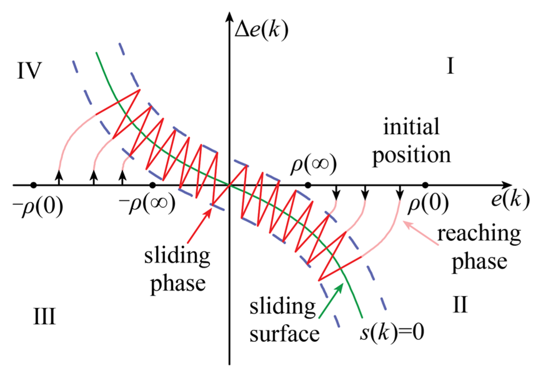
where λ₁ and λ₂ are normal constants, while λ₃ is the ratio of two odd numbers, satisfying 0 < λ₃ < 1. The phase plane diagram of the proposed sliding surface is illustrated in Figure 1. The control objective is to design a controller that constrains e(k) within the interval defined by Equation (28) and drives it to converge to zero. As shown in Figure 1, the boundaries of the sliding motion for the sliding surface intersect with the horizontal axis between ρ_∞ and −ρ_∞ in Regions I and III, respectively. The initial error range is bounded by [−ρ₀, ρ₀], ensuring that the tracking error always remains within the prescribed performance boundaries.

Figure 1. The phase plane of FITSMC.

Therefore, $s(k+1)$ is designed as follows:

$$\begin{array}{cc}\hfill s(k+1)& =\phi \left(k+1\right)+{\lambda }_1{\displaystyle \sum _{i=0}^k\phi \left(i\right)}+{\lambda }_2{\displaystyle \sum _{i=0}^k{\phi }^{{\lambda }_3}\left(i\right)}\hfill \\ & ={\displaystyle \frac{\pi e\left(k+1\right)}{2\rho \left(k+1\right)}}+{\lambda }_1{\displaystyle \sum _{i=0}^k\phi \left(i\right)}+{\lambda }_2{\displaystyle \sum _{i=0}^k{\phi }^{{\lambda }_3}\left(i\right)}\hfill \end{array}$$

(34)

Let $s(k+1)=0$, from Equation (34), it follows that

$$e\left(k+1\right)=-{\displaystyle \frac{2\rho \left(k+1\right)}{\pi }}\left({\lambda }_1{\displaystyle \sum _{i=0}^k\phi \left(i\right)}+{\lambda }_2{\displaystyle \sum _{i=0}^k{\phi }^{{\lambda }_3}\left(i\right)}\right)$$

(35)

The control input signal $u_{m,0}\left(k\right)$ is designed as follows:

$$u_{m,0}(k)=u_m(k-1)+\Delta u_m(k)$$

(36)

where $\Delta u_m(k)$ consists of the equivalent control law $\Delta u_m^{eq}(k)$ and the switching control law $\Delta u_m^{sc}(k)$, represented as follows:

$$\Delta u_m(k)=\Delta u_m^{eq}(k)+\Delta u_m^{sc}(k)$$

(37)

By combining Equation (27) and Equation (35), $\Delta u_m^{eq}(k)$ can be derived as follows:

$$\begin{array}{cc}\hfill \Delta u_m^{eq}(k)& ={\displaystyle \frac{1}{\widehat{\Phi }(k)+R}}\left(y_r\left(k+1\right)-y_d\left(k\right)+{\displaystyle \frac{2\rho \left(k+1\right)}{\pi }}\left({\lambda }_1{\displaystyle \sum _{i=0}^k\phi \left(i\right)}+{\lambda }_2{\displaystyle \sum _{i=0}^k{\phi }^{{\lambda }_3}\left(i\right)}\right)\right.\hfill \\ & \left.-\widehat{\zeta }\left(k\right)-{\beta }_{o}o\left(k\right)\right)\hfill \end{array}$$

(38)

To guarantee finite-time convergence to the sliding mode surface, overcome the drawbacks of traditional reaching laws, and avoid chattering when reaching the sliding mode surface, $\Delta u_m^{sc}(k)$ is designed as follows:

$$\Delta u_m^{sc}(k)={\displaystyle \frac{1}{\widehat{\Phi }(k)+R}}\left(\tau \left(s(k)\right)\mathrm{sign}\left(s(k)\right)\right.\left.-{\tau }_{2}s(k)\right)$$

(39)

where $\tau \left(s(k)\right)={\tau }_1\left|s(k)\right|+{\sigma }_{\mathrm{o}}$, ${\tau }_1$, ${\sigma }_{\mathrm{o}}$, ${\tau }_2$ are all positive real numbers, and ${\tau }_2-1<{\tau }_1<{\tau }_2+1$, ${\sigma }_{\mathrm{o}}>\left|\tilde{\zeta }(k)\right|$, $0<{\tau }_2<1$.

Remark 3.

From Equation (39), it can be seen that the reaching law achieves dual optimization through dynamic gain adjustment: it accelerates convergence when far from the sliding surface to improve the reaching speed and automatically decelerates near the sliding surface to suppress chattering, thereby balancing the rapid response with control smoothness.

Thus, the system controller is designed as follows:

$$\begin{array}{cc}\hfill u_{m,0}(k)& =u_m(k-1)+{\displaystyle \frac{1}{\widehat{\Phi }(k)+R}}\left(y_r\left(k+1\right)-y_d\left(k\right)+{\displaystyle \frac{2\rho \left(k+1\right)}{\pi }}\left({\lambda }_1{\displaystyle \sum _{i=0}^k\phi \left(i\right)}+{\lambda }_2{\displaystyle \sum _{i=0}^k{\phi }^{{\lambda }_3}\left(i\right)}\right)\right.\hfill \\ & -\widehat{\zeta }\left(k\right)-{\beta }_{o}o\left(k\right)+\tau \left(s(k)\right)\mathrm{sign}\left(s(k)\right)\left.-{\tau }_{2}s(k)\right)\hfill \end{array}$$

(40)

The Sat(⋅) function is defined as follows:

$$u_m(k)=\mathrm{Sat}\left\{\left(u_m(k-1)+\mathrm{Sat}\left\{\left(u_{m,0}(k)-u_m(k-1)\right),\right.\right.\right.\left.\left.T_s{\overline{u}}_{m\min }(k),T_s{\overline{u}}_{m\max }(k)\right\}\right),\left.u_{m\min },u_{m\max }\right\}$$

(41)

where u_{m max} and u_{m min} are the upper and lower bounds of the Sat(·) function.

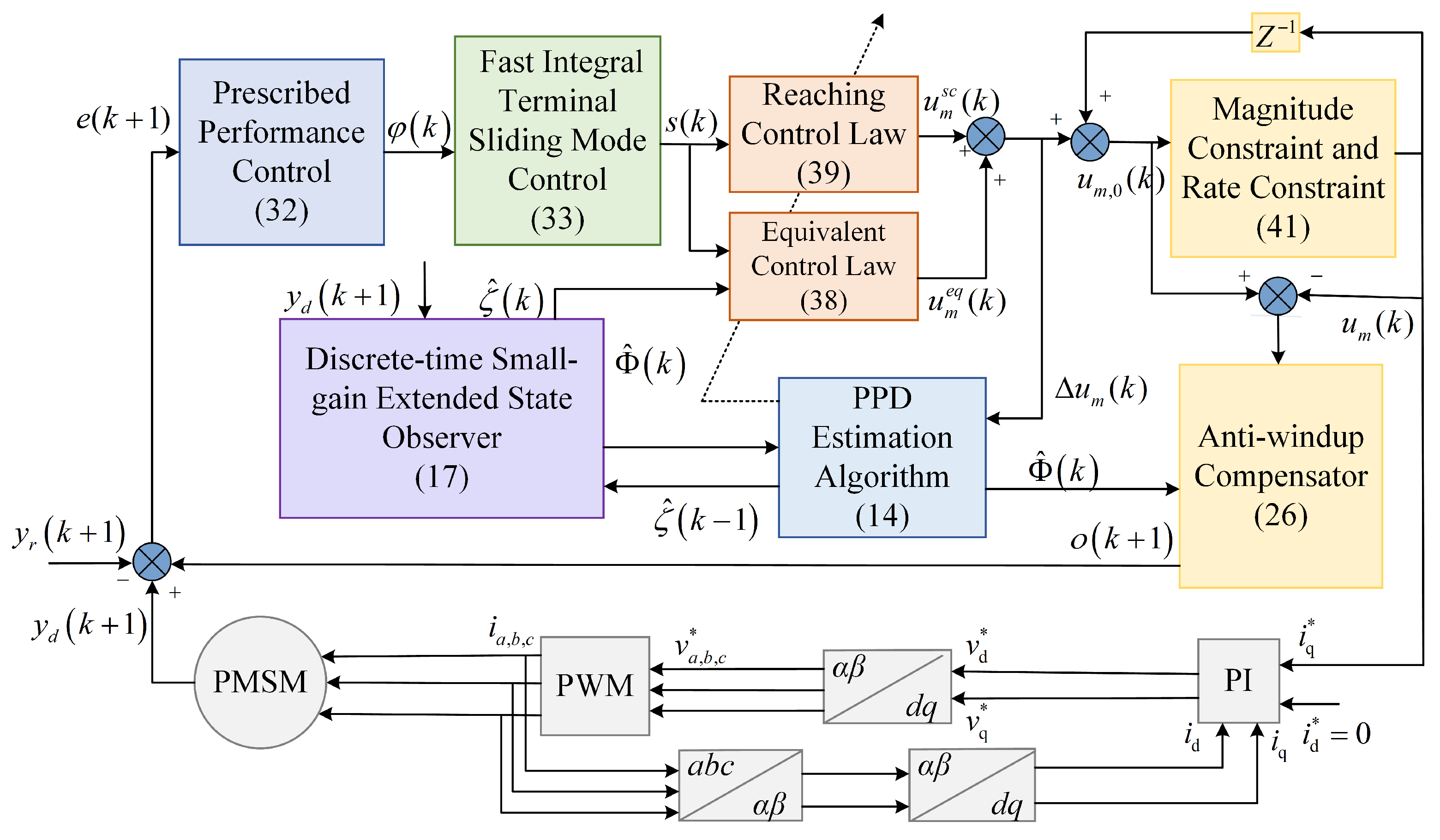
In summary, the control block diagram of the PP-MFA-FITSMC for the PMSM is shown in Figure 2.

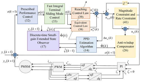
Figure 2. The control block diagram of the PP-MFA-FITSMC method of PMSM.

3.6. System Convergence Analysis

Lemma 1

([27]). For the discrete SMC systems, the necessary and sufficient condition for reachability is as follows:

$$\left\{\begin{array}{l}\left[s_e(k+1)-s_e(k)\right]\mathrm{sign}\left(s_e(k)\right)<0\\ \left[s_e(k+1)+s_e(k)\right]\mathrm{sign}\left(s_e(k)\right)>0\end{array}\right.$$

(42)

If the above inequality (42) holds, s_e(k) will asymptotically converge to the sliding surface.

Lemma 2

([26]). The following system is considered:

$$h(k+1)=h(k)-{\eta }_1{h}^m(k)-{\eta }_{2}h(k)+\alpha (k)$$

(43)

where η₁ > 0, 0 < η₂ < 1, 0 < m < 1. If the variable $\left|{\alpha }_0(k)\right|<{\overline{\alpha }}_0$ , then the system state h(k) will gradually converge into the following domain in a finite time:

$$\left\{h(k)\left|\left|h(k)\right|\right.\le \left(1+m^{{\displaystyle \frac{m}{1-m}}}-m^{{\displaystyle \frac{1}{1-m}}}\right)\cdot \max \left\{{\left({\displaystyle \frac{\overline{\alpha }}{{\eta }_1}}\right)}^{{\displaystyle \frac{1}{m}}},{\left({\displaystyle \frac{{\eta }_1}{1-{\eta }_2}}\right)}^{{\displaystyle \frac{1}{1-m}}}\right\}\right\}$$

(44)

Theorem 1.

Consider Equation (5) that satisfies assumptions 1, 2, and 3. Assuming ρ₀(k) < e₀(k) < ρ₀(k) holds, the control method proposed in this paper, as described by Equation (41), ensures that the position error e(k) is constrained within the prescribed boundaries and that the estimation error $\tilde{\zeta }\left(k\right)$ is bounded with respect to the sliding surface s(k).

Proof. 

1. Boundedness of the DSGESO estimation error

From Equation (19), the DSGESO observation error can be transformed as follows:

$$\tilde{X}(k+1)=\tilde{A}\tilde{X}(k)+{\tilde{E}}_1\tilde{\Phi }(k)\Delta u_m(k)+{\tilde{E}}_2\Delta \tilde{\zeta }\left(k\right)$$

(45)

where $\tilde{A}=\left[\begin{array}{cc}1-T_s{l}_{o1}& 1\\ 0& 1-T_s{l}_{o2}\end{array}\right]$.

Therefore, the nominal system of Equation (45) can be defined as follows:

$$\tilde{X}(k+1)=\tilde{A}\tilde{X}(k)$$

(46)

The designed DSGESO is stable only when all the eigenvalues of the matrix $\tilde{A}$ are located within the unit circle. The characteristic polynomial of $\tilde{A}$ is derived as follows:

$$\begin{array}{cc}\hfill \left|zI-\tilde{A}\right|& =\left[\begin{array}{cc}z-1+T_s{l}_{o1}& -1\\ 0& z-1+T_s{l}_{o2}\end{array}\right]\hfill \\ & =z^2+\left(T_s{l}_{o1}+T_s{l}_{o2}-2\right)z+\left(T_s^2{l}_{o1}{l}_{o2}-T_s{l}_{o1}-T_s{l}_{o2}+1\right)\hfill \end{array}$$

(47)

By substituting z = (w + 1)/(w − 1) into Equation (47), the characteristic polynomial can be obtained:

$$T_s^2{l}_{o1}{l}_{o2}{w}^2+\left(2T_s{l}_{o1}+2T_s{l}_{o2}-2T_s^2{l}_{o1}{l}_{o2}\right)w+\left(T_s^2{l}_{o1}{l}_{o2}-2T_s{l}_{o1}-2T_s{l}_{o2}+4\right)=0$$

(48)

According to the Routh criterion, the condition for the stability of the matrix $\tilde{A}$ is as follows:

$$\left\{\begin{array}{l}{T}_s^2{l}_{o1}{l}_{o2}>0\hfill \\ 2T_s{l}_{o1}+2T_s{l}_{o2}-2T_s^2{l}_{o1}{l}_{o2}>0\hfill \\ T_s^2{l}_{o1}{l}_{o2}-2T_s{l}_{o1}-2T_s{l}_{o2}+4>0\hfill \end{array}\right.$$

(49)

Due to the observer gains $l_{o1}=l_{o2}={\omega }_o>0$, substituting into Equation (49) yields

$$\left\{\begin{array}{l}{T}_s^2{\omega }_o^2>0\hfill \\ T_s{\omega }_o<2\hfill \\ {\left(T_s{\omega }_o-2\right)}^2>0\hfill \end{array}\right.$$

(50)

Therefore, when $T_s{\omega }_0<2$, the system is globally asymptotically stable. It is deduced that

$$\left\{\begin{array}{l}\underset{k\to \infty }{\lim }{\tilde{y}}_d\left(k\right)={\displaystyle \frac{\tilde{\zeta }\left(k\right)+\tilde{\Phi }(k)\Delta u_m(k)}{T_s{\omega }_o}}\hfill \\ \underset{k\to \infty }{\lim }\tilde{\zeta }\left(k\right)={\displaystyle \frac{\Delta \zeta \left(k\right)}{T_s{\omega }_o}}\hfill \end{array}\right.$$

(51)

From Assumption 4, $\left|\Delta \zeta \left(k\right)\right|\le b$, and then it follows that

$$\left\{\begin{array}{l}\left|{\tilde{y}}_d\left(k\right)\right|\le {\displaystyle \frac{b}{T_s^2{\omega }_o^2}}+{\displaystyle \frac{\tilde{\Phi }(k)\Delta u_m(k)}{T_s{\omega }_o}}={\sigma }_1\hfill \\ \left|\tilde{\zeta }\left(k\right)\right|\le {\displaystyle \frac{b}{T_s{\omega }_o}}={\sigma }_2\hfill \end{array}\right.$$

(52)

Thus, $\tilde{X}(k)$ is bounded, and then, $\widehat{\zeta }\left(k\right)$ is also bounded.

2. Boundedness of s(k)

Substituting Equations (27) and (40) into Equation (34) yields

$$s(k+1)={\displaystyle \frac{\pi }{2\rho \left(k+1\right)}}\left(-\tau \left(s(k)\right)\mathrm{sign}\left(s(k)\right)-\tilde{\zeta }\left(k\right)+{\tau }_{2}s(k)\right)$$

(53)

From Equation (53), it can be concluded that

$$\begin{array}{c}\left[s(k+1)-s(k)\right]\mathrm{sign}\left(s(k)\right)\hfill \\ ={\displaystyle \frac{\pi }{2\rho (k+1)}}\left[\left({\tau }_2-1-{\tau }_1\right)\left|s(k)\right|-{\sigma }_{\mathrm{o}}-\tilde{\zeta }\left(k\right)\mathrm{sign}\left(s(k)\right)\right]\hfill \\ <0\hfill \end{array}$$

(54)

where the parameters of the controller in Inequality (54) satisfy the following inequalities:

$$\left\{\begin{array}{l}{\tau }_1>{\tau }_2-1\\ -{\sigma }_{\mathrm{o}}-\tilde{\zeta }\left(k\right)\mathrm{sign}\left(s(k)\right)<0\end{array}\right.$$

(55)

Next,

$$\begin{array}{c}\left[s(k+1)+s(k)\right]\mathrm{sign}\left(s(k)\right)\hfill \\ ={\displaystyle \frac{\pi }{2\rho (k+1)}}\left[\left({\tau }_2+1-{\tau }_1\right)\left|s(k)\right|-{\sigma }_{\mathrm{o}}-\tilde{\zeta }\left(k\right)\mathrm{sign}\left(s(k)\right)\right]\hfill \\ >{\displaystyle \frac{\pi }{2\rho (+\infty )}}\left[\left({\tau }_2+1-{\tau }_1\right)\left|s(k)\right|-2{\sigma }_{\mathrm{o}}\right]\hfill \end{array}$$

(56)

where the parameters of the controller in Inequality (56) satisfy the following inequalities:

$$\left\{\begin{array}{l}{\tau }_1<{\tau }_2+1\\ -{\sigma }_{\mathrm{o}}-\tilde{\zeta }\left(k\right)\mathrm{sign}\left(s(k)\right)>-2{\sigma }_{\mathrm{o}}\end{array}\right.$$

(57)

Define $\Lambda ={\displaystyle \frac{2{\sigma }_o}{{\tau }_2+1-{\tau }_1}}$; then, from Inequality (56), it can be concluded that [s(k + 1) + s(k)]sign(s(k)) > 0 holds if and only if the following inequality is satisfied:

$$\left|s(k)\right|>\Lambda$$

(58)

This is equivalent to

$$s(k)>\Lambda \mathrm{or}s(k)<-\Lambda$$

(59)

Accordingly, define the bounded region as follows:

$${\Theta }_2\triangleq \left\{s(k)\left|-\Lambda \le s(k)\le \Lambda \right.\right\}$$

(60)

When $s(k)\notin {\Theta }_2$ holds, that is, when Inequality (58) is satisfied, the reachability condition of the sliding mode surface is fulfilled. Therefore, s(k) will gradually converge to the region ${\Theta }_2$. Once $s(k)\in {\Theta }_2$, $s(k)$ will always hold:

$$\left|s(k)\right|\le \Lambda$$

(61)

This leads to

$$\underset{k\to +\infty }{\lim }\left|s(k)\right|\le \Lambda$$

(62)

According to the above analysis, the sliding mode surface converges to a bounded region.

3. Boundedness of the output error e(k)

From Equations (33) and (34), it can be seen that

$$s(k+1)-s(k)=\phi (k+1)+{\lambda }_2{\phi }^{{\lambda }_3}(k)+\left({\lambda }_1-1\right)\phi (k)$$

(63)

From this, it follows that

$$\begin{array}{cc}\hfill \phi (k+1)& =\phi (k)-{\lambda }_2{\phi }^{{\lambda }_3}(k)-{\lambda }_1\phi (k)+\left(s(k+1)-s(k)\right)\hfill \\ & =\phi (k)-{\lambda }_2{\phi }^{{\lambda }_3}(k)-{\lambda }_1\phi (k)+{\omega }_1(k)\hfill \end{array}$$

(64)

where

$${\omega }_1(k)\triangleq s(k+1)-s(k)\le \left|s(k+1)\right|+\left|s(k)\right|$$

(65)

From Inequality (64) and Equation (65), it can be obtained that ${\omega }_1(k)$ is bounded, satisfying the following:

$$\underset{k\to +\infty }{\lim }\left|{\omega }_1(k)\right|\le \underset{k\to +\infty }{\lim }\left(\left|s(k+1)\right|+\left|s(k)\right|\right)\le 2\Lambda$$

(66)

Combining with Lemma 2, it can be concluded that

$$\underset{k\to \infty }{\lim }\left|\phi \left(k\right)\right|\le \left({1+{\lambda }_3}^{{\displaystyle \frac{{\lambda }_3}{1-{\lambda }_3}}}-{{\lambda }_3}^{{\displaystyle \frac{1}{1-{\lambda }_3}}}\right)\times \max \left\{{\left({\displaystyle \frac{2\Lambda }{{\lambda }_2}}\right)}^{{\displaystyle \frac{1}{{\lambda }_3}}},{\left({\displaystyle \frac{{\lambda }_2}{1-{\lambda }_1}}\right)}^{{\displaystyle \frac{1}{1-{\lambda }_3}}}\right\}$$

(67)

By appropriately choosing parameters ${\lambda }_1,{\lambda }_2$, and ${\lambda }_3$, it can be ensured that inequality (67) satisfies $\underset{k\to \infty }{\lim }\left|\phi \left(k\right)\right|\le {\displaystyle \frac{\pi }{2}}$. The variable $\phi (k)$ gradually reaches and enters the bounded set ${\Theta }_1$ through suitable parameters. Therefore, e(k) is always confined within the predefined adjustable domain.

4. The boundedness of $\widehat{\Phi }(k)$

Let $\tilde{\Phi }(k)=\widehat{\Phi }(k)-\Phi (k)$, where $\tilde{\Phi }(k)$ is the estimation error of $\Phi (k)$. Subtracting $\Phi (k)$ from both sides of Equation (14) yields the following:

$$\tilde{\Phi }(k)=\widehat{\Phi }(k-1)\left[1-{\displaystyle \frac{\kappa \Delta u_m(k-1)\Delta u_m(k-1)}{\chi +\Delta u_m{(k-1)}^2}}\right]-{\displaystyle \frac{\kappa \tilde{\zeta }(k-1)\Delta u_m(k-1)}{\chi +\Delta u_m{(k-1)}^2}}+\Phi (k)-\Phi (k-1)$$

(68)

where since $‖\Phi (k)‖\le a$, then $‖\Phi (k)-\Phi (k-1)‖\le 2a$, and then $‖{\displaystyle \frac{\kappa \tilde{\zeta }(k-1)\Delta u_m(k-1)}{\chi +\Delta u_m{(k-1)}^2}}‖\le \kappa {\displaystyle \frac{b}{2\sqrt{\chi }}}$ and $\left|\tilde{\Phi }(k-1)\left(1-{\displaystyle \frac{\kappa \Delta u_m(k-1)\Delta u_m(k-1)}{\chi +\Delta u_m{(k-1)}^2}}\right)\right|\le A_1\left|\tilde{\Phi }(k-1)\right|$ can be derived, where A₁ ≤ 1; therefore, by applying the absolute value to Inequality (68), the following can be obtained:

$$\begin{array}{c}|\tilde{\Phi }(k)|\le A_1|\tilde{\Phi }(k-1)|+\kappa {\displaystyle \frac{b}{2\sqrt{\chi }}}+2a\hfill \\ \le A_1^2|\tilde{\Phi }(k-2)|+A_1\left(\kappa {\displaystyle \frac{b}{2\sqrt{\chi }}}+2a\right)+\kappa {\displaystyle \frac{b}{2\sqrt{\chi }}}+2a\hfill \\ \le \cdots \le A_1^{k-1}|\tilde{\Phi }(1)|+\left(\kappa {\displaystyle \frac{b}{2\sqrt{\chi }}}+2a\right)\left({\displaystyle \frac{1-A_1^{k-1}}{1-A_1}}\right)\hfill \end{array}$$

(69)

Obviously, the PPD estimation error $\tilde{\Phi }(k)$ is bounded and $\widehat{\Phi }(k)$ is bounded and convergent.

Proof end. □

4. Experimental Validation

4.1. Platform Overview

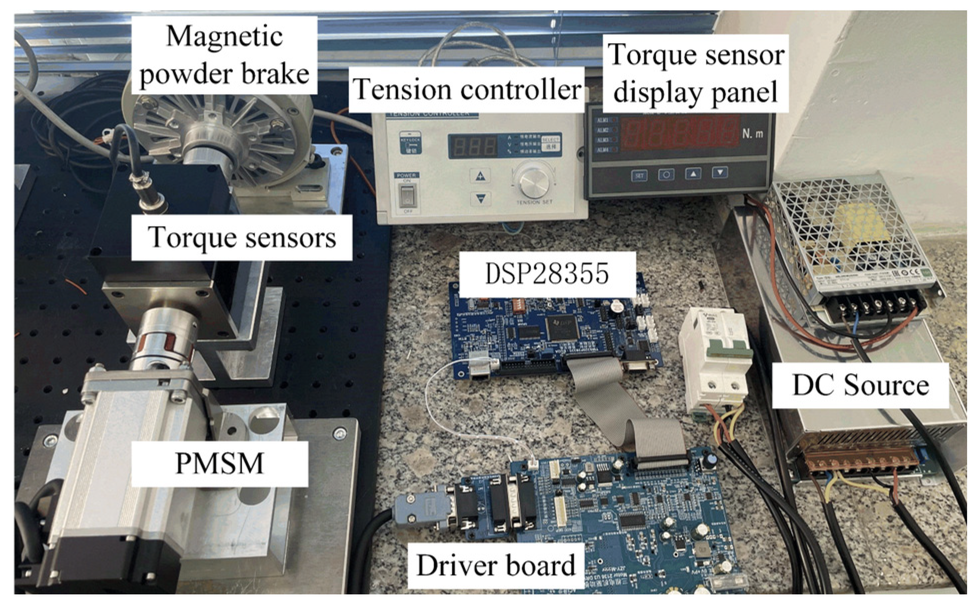
To further evaluate the position control performance of the PP-MFA-FITSMC method, the PMSM position control experimental platform was designed and built based on the schematic in Figure 2. The constructed experimental platform is shown in Figure 3, and the PMSM parameters are listed in Table 1. The experimental platform downloads the control method designed in Matlab R2024a/Simulink to the TMS320F28335-EU2A main control board via Code Composer Studio. The main control board sends position commands to the driver board through the RS485 communication protocol to drive the PMSM. The experimental platform uses a magnetic powder brake combined with a tension controller to simulate the load, an encoder measures the position of the test rig, and a torque sensor detects the motor torque. The measured data are fed back to the main control board to form a closed-loop control system.

Figure 3. PMSM experimental platform.

Table 1. PMSM Parameters.

Paraments	Values
ψf	0.0167 Wb
Rs	0.32 Ω
Lo	0.64 mH
P	2
Rated torque	1.27 N·m
J	0.000028 kg·m2

4.2. Controller Parameter Sensitivity Analysis

Due to the limitations imposed by the complexity of dynamic models based on controller tuning methods, incorporating statistically designed experimental schemes can reduce the number of trials while improving the accuracy of fitted models. The response surface methodology not only investigates the interaction effects and provides optimization information but also visually demonstrates functional relationships through response surface plots [28,29]. In this study, the Box–Behnken Design (BBD) algorithm from the response surface analysis is employed to examine the influence of selected controller parameters on system performance. In the experiment, the tracking error of the system was constrained within predefined bounds via PPC. To prevent significant system failures, appropriate relaxation of the error bounds was implemented. A step position command of 6 rad was applied as the reference input, with additional disturbances including a 0.1 N·m sinusoidal time-varying load torque and measurement noise represented by m(k) = 0.1 rand(1). The system’s performance was evaluated based on two key indicators: the settling time (for rapidity assessment) and steady-state error range (for stability evaluation). Parameters $\widehat{\Phi }\left(1\right)$, $\chi$, T_sl_o1, λ₁, and λ₂ are chosen as independent variables, represented by A, B, C, D, and E, respectively, as shown in Table 2. Building upon empirical methods, three distinct numerical values with coded levels are assigned to each independent variable. The settling time (ΔT) and steady-state error range (ΔE_s) under step signal conditions are selected as response variables.

Table 2. Parameters and numerical range of response surface.

Independent Variable	level
	−1	0	1
A	2	16	30
B	100	250	400
C	0.5	1	1.5
D	0.4	0.65	0.9
E	100	1550	3000

Since polynomial approximation models represent one of the common approaches for establishing relationships between objectives and variables, a second-order response model was selected to approximate the response function during the design of variables. The fundamental model is expressed as follows:

$$y(x)={\beta }_0+{\displaystyle \sum _{i=1}^k{\beta }_i{x}_i}+{\displaystyle \sum _{i=1}^k{\beta }_{ii}}{x}_i^2+{\displaystyle \sum _{i<j}^k{\beta }_{ij}}{x}_i{x}_j+\iota$$

(70)

where y(x) is the objective function, x_i is the i-th independent variable, β_i is the linear effect coefficient of x_i, β_ii is the quadratic effect coefficient of x_i, β_ij is the interaction effect coefficient between x_i and x_j, and $\iota$ is the residual error.

When using settling time as the response variable, Design-Expert12 software was employed to perform an analysis of variance on the results. This study adopted a linear regression model to establish the relationship between various factors and the recovery efficiency. Through a statistical analysis of the experimental data and processing via the software, a second-order regression equation was obtained as follows:

$$\begin{array}{cc}\hfill \Delta T& =0.16-1.30\times {10}^{-3}\mathrm{A}+8.45\times {10}^{-4}\mathrm{B}-0.03\mathrm{C}-5.35\times {10}^{-3}\mathrm{D}-2.68\times {10}^{-6}\mathrm{E}\hfill \\ & -5.11\times {10}^{-6}\mathrm{AB}+6.42\times {10}^{-4}\mathrm{AC}+2.89\times {10}^{-4}\mathrm{AD}+8.22\times {10}^{-7}\mathrm{AE}\hfill \\ & -5.83\times {10}^{-6}\mathrm{BC}-8.56\times {10}^{-5}\mathrm{BD}-1.31\times {10}^{-7}\mathrm{BE}+4.25\times {10}^{-3}\mathrm{CD}\hfill \\ & +3.00\times {10}^{-6}\mathrm{CE}-4.78\times {10}^{-6}\mathrm{DE}-3.60\times {10}^{-5}{\mathrm{A}}^2-1.04\times {10}^{-6}{\mathrm{B}}^2\hfill \\ & +1.38\times {10}^{-3}{\mathrm{C}}^2+5.49\times {10}^{-3}{\mathrm{D}}^2+3.27\times {10}^{-9}{\mathrm{E}}^2\hfill \end{array}$$

(71)

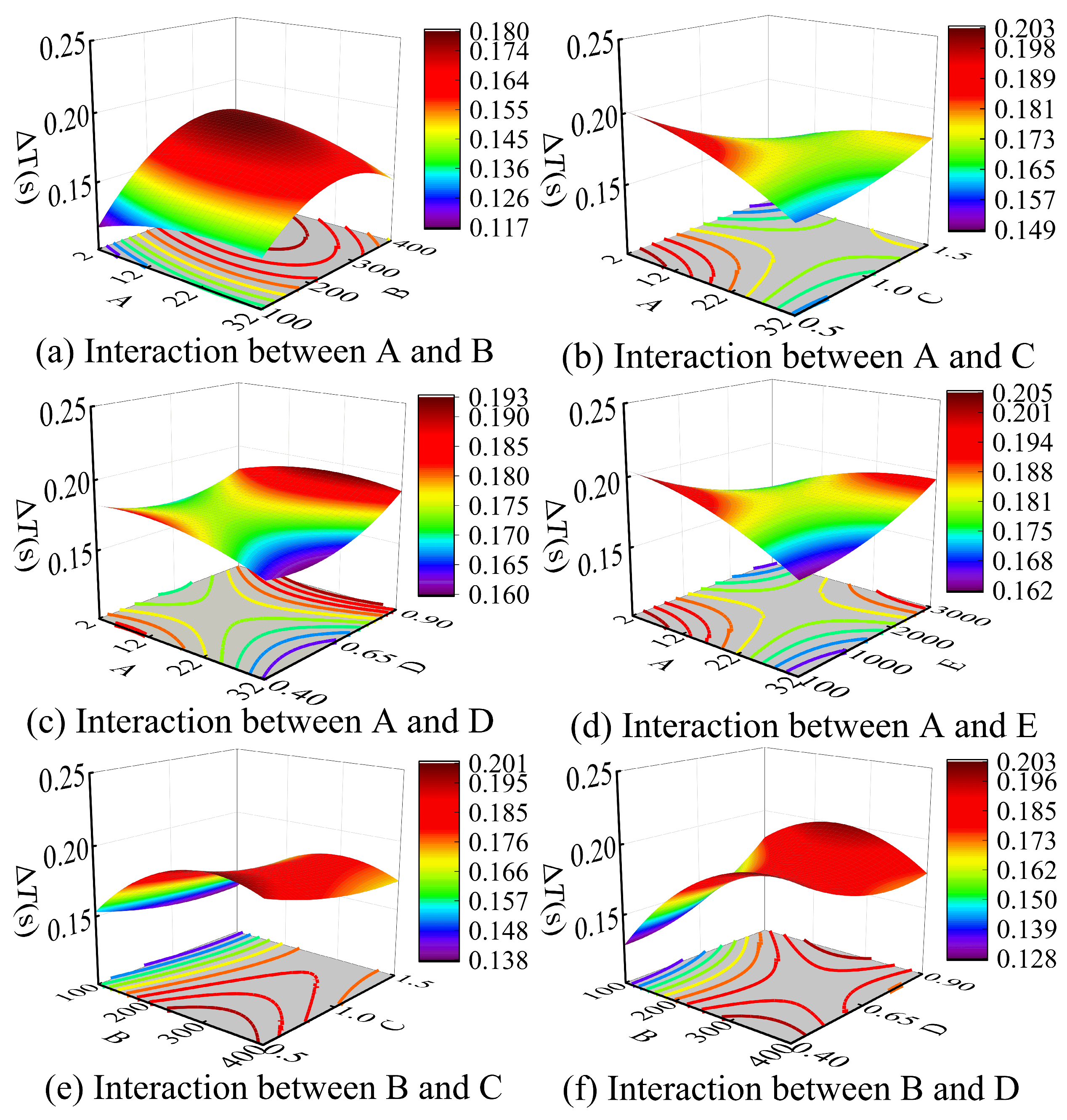
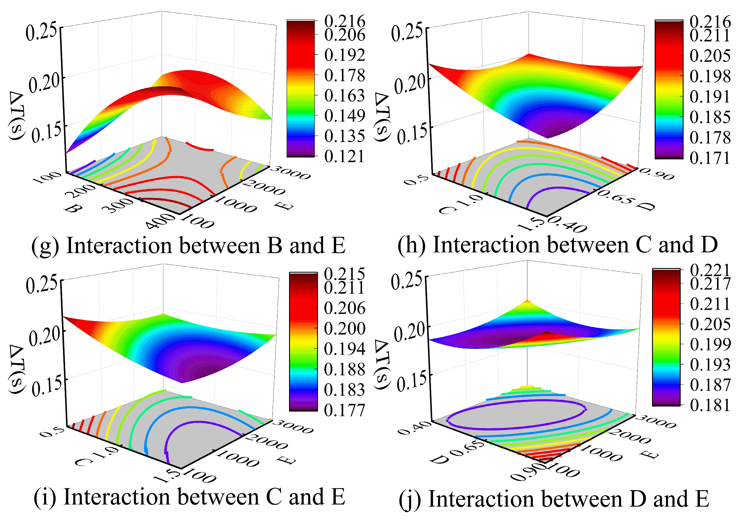
A statistical analysis using settling time as the dependent variable yielded significant results: the model’s null hypothesis probability p = 0.0395 < 0.05 confirmed the significance of the influencing factors, while the lack-of-fit term p = 0.3027 > 0.05 proved statistically insignificant. The model’s overall F-value of 2.15 demonstrated statistical significance, with individual factor F-values ranking as F_B = 8.15 > F_C = 2.07 > F_D = 0.8867 > F_A = 0.2359 > F_E = 0.107, indicating their relative influence on the stabilization time. An interaction analysis conducted via Design-Expert generated the three-dimensional response surface plots shown in Figure 4, illustrating pairwise variable interactions. As shown in Figure 4, the interaction between parameters B and E constitutes the primary factor influencing the system settling time, while the interaction between A and D demonstrates a minimal impact. Taking the B and E interaction presented in Figure 4g as a specific case, when maintaining other parameters constant and adjusting solely B and E values, the system settling time varies within the range of [0.121, 0.216] s. The minimal settling time of 0.121 s occurs when both parameters B and E are set at lower values. Conversely, two suboptimal scenarios emerge: (1) when E is small but B is large, or (2) when E is large but B is small—both configurations result in prolonged settling times. Most notably, when both B and E assume larger values simultaneously, the system exhibits significantly degraded performance with settling times increased by 78.5% compared to the optimal case where both parameters are minimized.

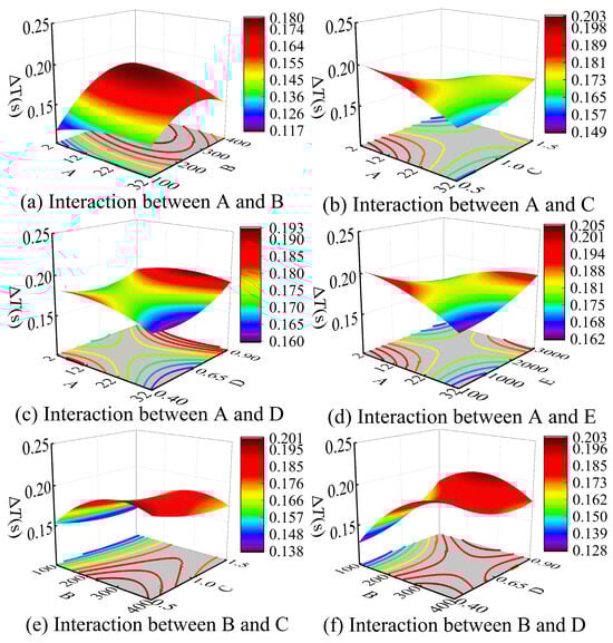
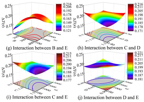
Figure 4. Effects of independent variables on the system settling time.

When steady-state error was selected as the response variable, the derived second-order regression equation was obtained as follows:

$$\begin{array}{cc}\hfill \Delta E_{\mathrm{s}}& =12.81-0.22\mathrm{A}-0.026\mathrm{B}+1.53\mathrm{C}-3.01\mathrm{D}+2.04\times {10}^{-3}\mathrm{E}+1.57\times {10}^{-3}\mathrm{AB}\hfill \\ & -0.12\mathrm{AC}+0.0630\mathrm{AD}-2.1\times {10}^{-5}\mathrm{AE}-1.92\times {10}^{-3}\mathrm{BC}+1.11\times {10}^{-3}\mathrm{BD}\hfill \\ & -3.56\times {10}^{-6}\mathrm{BE}+0.46\mathrm{CD}-1.00\times {10}^{-3}\mathrm{CE}-3.22\times {10}^{-4}\mathrm{DE}+4.32\times {10}^{-3}{\mathrm{A}}^2\hfill \\ & +4.90\times {10}^{-5}{\mathrm{B}}^2+0{.46\mathrm{C}}^2+0{.528\mathrm{D}}^2+1.02\times {10}^{-7}{\mathrm{E}}^2\hfill \end{array}$$

(72)

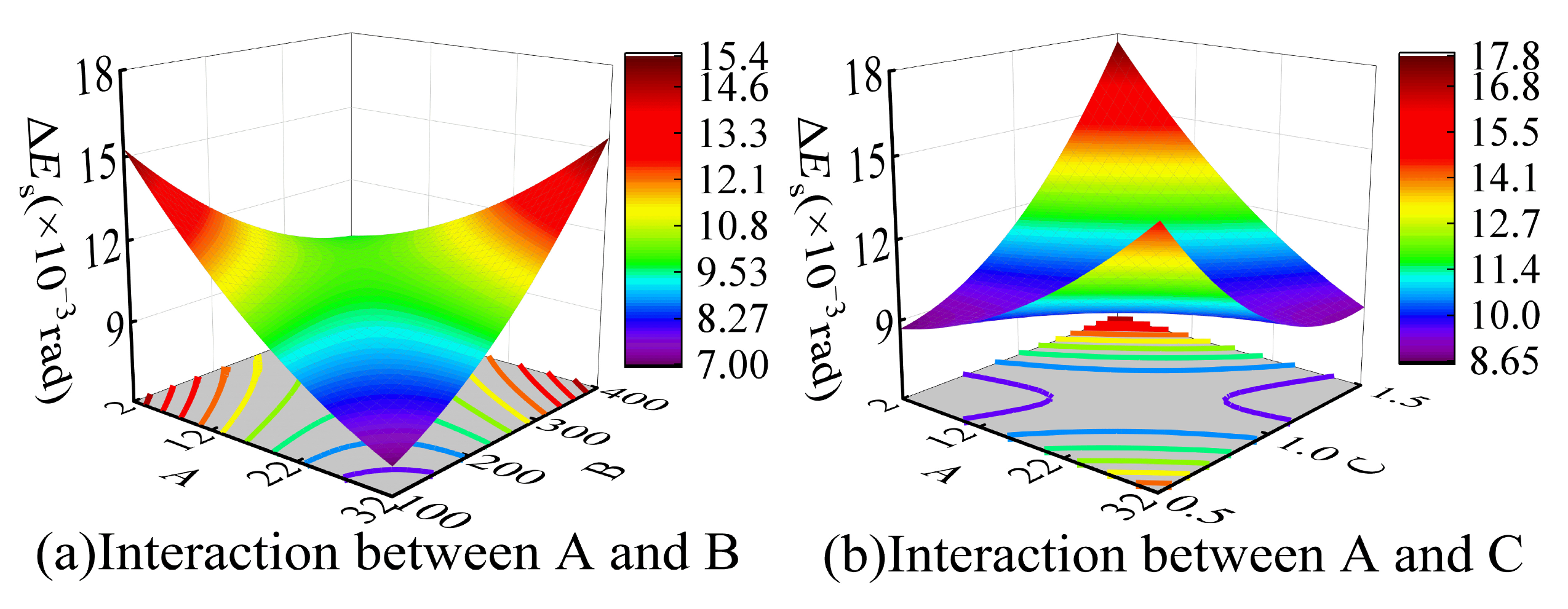
The analysis demonstrates that the model’s null hypothesis probability p = 0.0342 < 0.05 indicates statistically significant influencing factors, while the lack-of-fit term’s probability p = 0.3324 > 0.05 confirms its statistical insignificance. The model’s overall significance is evidenced by an F-value of 2.22, calculated as the ratio of the factor mean square to the error mean square, with individual factor F-values ranking as F_E = 6.14 > F_C = 1.83 > F_B = 1.31 > F_A = 1.06 > F_D = 0.0912, revealing their relative influence on the steady-state error range in descending order. An interaction analysis conducted via Design-Expert generated three-dimensional response surface plots shown in Figure 5, illustrating pairwise variable interactions. As shown in Figure 5, the interaction between parameters A and C constitutes the dominant factor affecting the steady-state error range, while the interaction between B and D exhibits the least influence. When steady-state error serves as the response variable, the effects of individual independent variables follow the same analytical methodology as demonstrated in Figure 4.

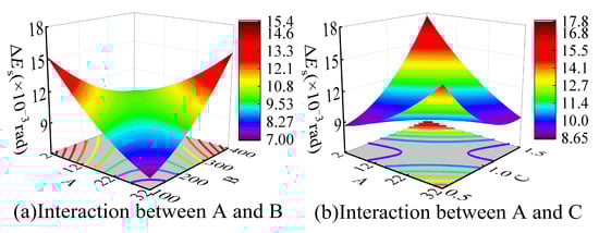
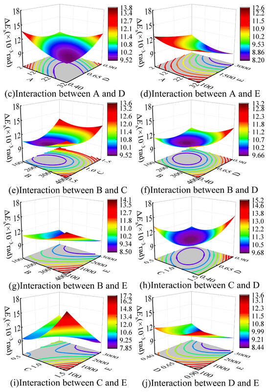
Figure 5. Effects of independent variables on steady-state error range.

Remark 4.

When the controller parameters are specified, it is difficult to observe a simple, consistent positive or negative correlation between the convergence rate and steady-state error. Their relationship is complex, nonlinear, and often mutually constraining. Parameter tuning constitutes a trade-off process that requires finding an acceptable balance point among several key performance objectives.

4.3. Performance Validation

To illustrate the superiority of the proposed controller, comparisons are made with PI control, DESO + MFAC, the disturbance observer-based nonlinear sliding mode control (DOB + NSMC) method in reference [8], PPC + FITSMC + MFAC, and the proposed PP-MFA-FITSMC method. The traditional DESO is designed with linear gains L = [l₁, l₂]^T. The parameters of the five control methods are obtained through a trial-and-error approach, taking system stability into full consideration. The specific parameter settings are shown in Table 3, and T_s = 0.1 ms.

Table 3. Parameters of controller.

Paraments	Values
PI (C1)	position loop: kp = 105, ki = 200 Speed loop: kp = 400, ki = 200
DESO + MFAC (C2)	l1 = 1, l2 = 0.2, $\widehat{\Phi }\left(1\right)=20$, R = 0.01, $\epsilon =0.001$, $\kappa =0.8$, $\chi =150$
Reference [8] DOB + NSMC (C3)	l = 300, k1 = 40, γ = 0.5, ρ = 40
PPC + FITSMC + MFAC (C4)	Sine wave signal: ρ0 = 0.015, ρ∞ = 0.0028, Step signal: ρ0 = 8, ρ∞ = 0.0028, θ1 = 1, ${\theta }_o=0.0001$, λ1 = 0.4, λ2 = 800, λ3 = 3/5, ${\tau }_1=0.01$, ${\sigma }_{\mathrm{o}}=0.5$, ${\tau }_2=0.5$, $\widehat{\Phi }\left(1\right)=20$, R = 0.01, $\epsilon =0.001$, $\kappa =0.8$, $\chi =150$
PP-MFA-FITSMC (C5)	${\omega }_0=8000$, θ1 = 1, θo = 0.0001. Sine wave signal: ρ0 = 0.015, ρ∞ = 0.0028, Step signal: ρ0 = 8, ρ∞ = 0.0028, λ1 = 0.4, λ2 = 800, λ3 = 3/5, ${\tau }_1=0.01$, ${\sigma }_{\mathrm{o}}=0.5$, ${\tau }_2=0.5$, $\widehat{\Phi }\left(1\right)=20$, R = 0.01, $\epsilon =0.001$, $\kappa =0.8$, $\chi =150$, βo = 0.1.

4.3.1. Experiment 1

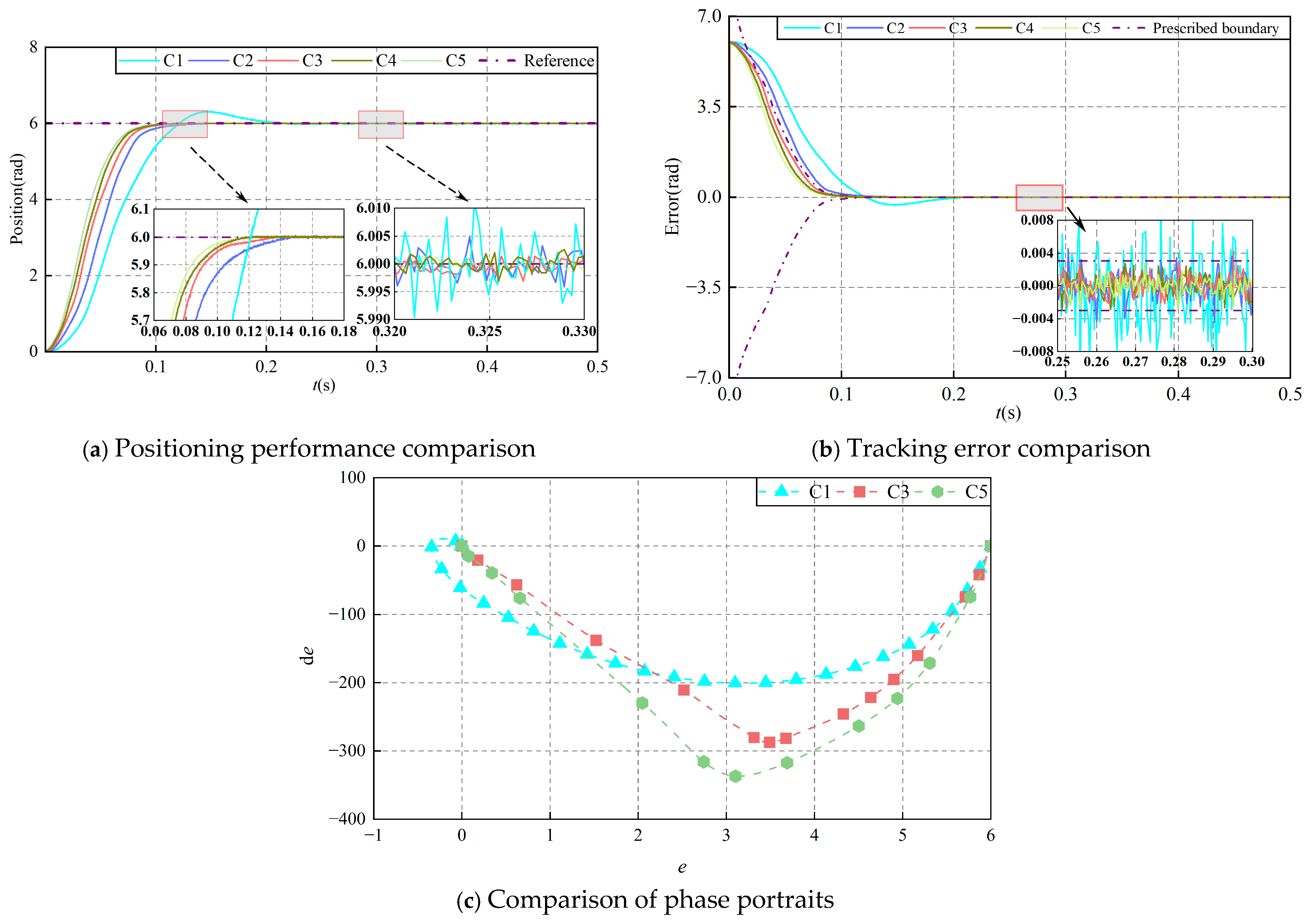
To verify the rapidity of the control method designed in this paper, a step position signal of 6 rad was given, and the motor was started under no-load conditions. Figure 6 shows the tracking results of the step position command under no load, and Table 4 presents the tracking error performance metrics of the step position command under no load. From Figure 6 and Table 4, it can be seen that the traditional C1 method has the worst tracking performance, with large overshoot and the longest settling time. The steady-state errors of C2 and C3 methods are also higher than those of C4 and C5 methods, indicating that the C5 method, when tracking the desired position command, stabilizes faster than other control schemes and has no overshoot. Both C4 and C5 methods maintain the system error within the set error boundaries. According to Table 4, the response time of the C5 method is 0.12 s, which is a decrease of 8.33% compared to C3 and C4 methods. The steady-state error of the C5 method is in the range of [−0.0026, 0.0020] rad, which is a reduction of 13.0% and 45.7% compared to C3 and C4 methods, respectively. Therefore, the C5 method exhibits the optimal position tracking control performance, with the fastest response speed and the smallest steady-state error. Figure 6c visually demonstrates that Method C1 exhibits overshoot and a longer settling time. In comparison, Method C3 significantly improves the convergence speed without any overshoot. Notably, the proposed Method C5 achieves smooth convergence with a faster convergence speed and higher stability.

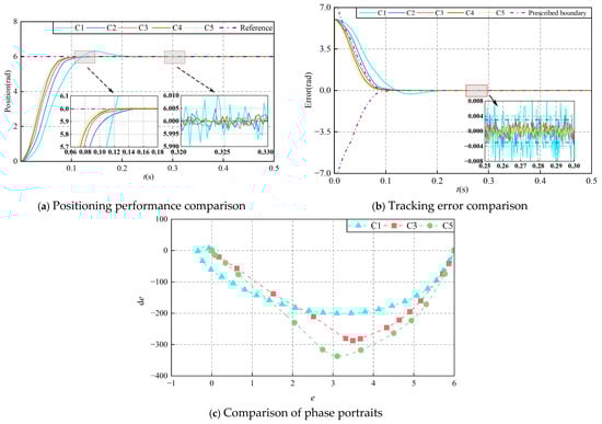
Figure 6. Operation result of step position command under no load.

Table 4. Tracking error performance metrics of step position command under no load.

Methods	Settling Time (s)	Overshoot (%)	Steady-State Error (Rad)
C1	0.21	5.05	[−0.0112, 0.0104]
C2	0.15	0	[−0.0072, 0.0065]
C3	0.13	0	[−0.0025, 0.0042]
C4	0.13	0	[−0.0027, 0.0025]
C5	0.12	0	[−0.0026, 0.0020]

4.3.2. Experiment 2

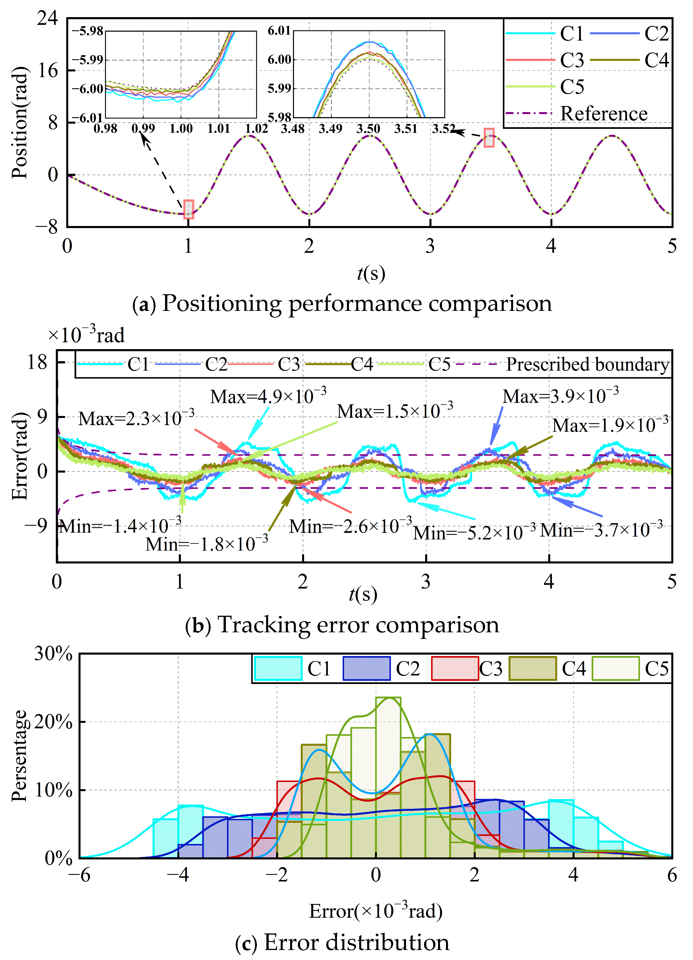
To verify the dynamic response performance of the proposed controller, during the no-load startup phase of the PMSM, a sine wave signal with a varying period and an amplitude of 6 rad is given. The tracking results under five control methods are shown in Figure 7, and selected the average error (e_ave), maximum error (e_max), and standard deviation (e_std) as evaluation metrics, as shown in Table 4. As seen in Figure 7 and Table 5, under no-load conditions, although methods C1 and C2 are able to track the desired position command, their tracking errors are relatively large. On the other hand, the tracking curves of the other methods show no significant lag. Although the tracking error is large in the initial phase of motor operation, it converges within a short period. When the motor stabilizes, method C3 has the most concentrated tracking error, followed by methods C3 and C4. The maximum tracking error for method C5 is 0.0015 rad, which is a reduction of 73.3% and 26.6% compared to methods C3 and C4, respectively. The standard deviation of the tracking error for method C5 is 2.5 rad, which is a reduction of 12.0% and 28.0% compared to methods C3 and C4, respectively. It can be concluded that method C2 provides a solid control performance foundation for methods C4 and C5. Method C5 not only successfully constrains all errors within the preset envelope to ensure its ideal prescribed performance but also provides the best dynamic performance.

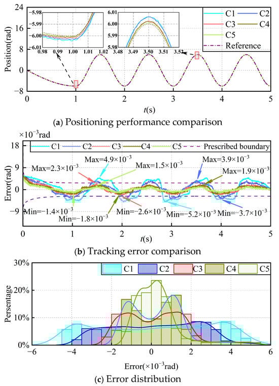
Figure 7. Operation result of sine position command under no load.

Table 5. Tracking error performance metrics of sine position command under no load.

Methods	eave (Rad)	emax (Rad)	estd (Rad)
C1	0.00074	0.0049	5.8
C2	0.00067	0.0039	4.4
C3	0.00052	0.0026	2.8
C4	0.00048	0.0019	3.2
C5	0.00037	0.0015	2.5

4.3.3. Experiment 3

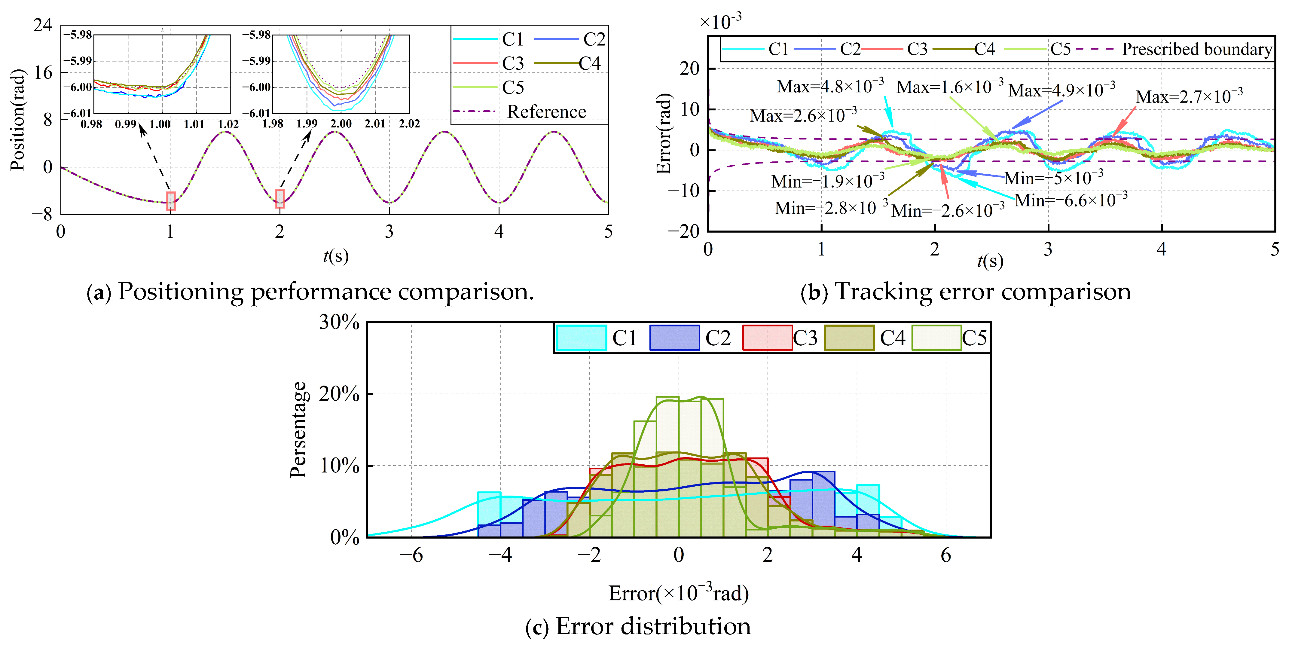
To verify the disturbance-suppression capability of the proposed control method for constant disturbances, a sine wave signal with a varying period and an amplitude of 6 rad is given, and a constant load of 0.2 N·m is applied at 2 s. The tracking results under five control methods are shown in Figure 8 and Table 6. As seen in Figure 8 and Table 6, after the sudden load is applied at 2 s, the tracking error shows small fluctuations. The maximum error of the C1 and C2 methods increases by 0.0017 rad and 0.0011 rad, respectively, indicating their poor robustness. The tracking error for the other methods shows no significant changes, but the overall tracking error stabilizes within a range of 0.003 rad. The maximum tracking error for the C5 method is 0.0019 rad, which is a reduction of 42.1% and 47.3% compared to the C3 and C4 methods, respectively. The standard deviation of the tracking error for the C5 method is 2.9 rad, which is a reduction of 10.3% and 6.9% compared to the C3 and C4 methods, respectively. The comparison shows that, when subjected to sudden disturbances, the proposed method in this paper offers better disturbance-suppression performance.

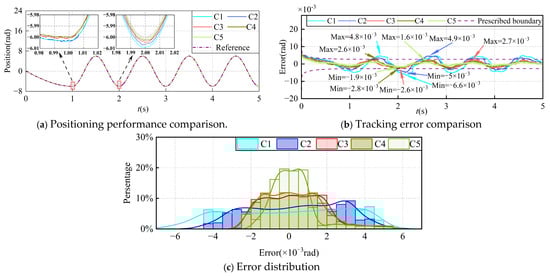
Figure 8. Operation result of sine position command under 0.2 N m constant load disturbance.

Table 6. Tracking error performance metrics of sine position command under 0.2 N m constant load disturbance.

Methods	eave (Rad)	emax (Rad)	estd (Rad)
C1	0.00078	0.0066	6.1
C2	0.00064	0.0050	4.8
C3	0.00061	0.0027	3.2
C4	0.00059	0.0028	3.1
C5	0.00050	0.0019	2.9

4.3.4. Experiment 4

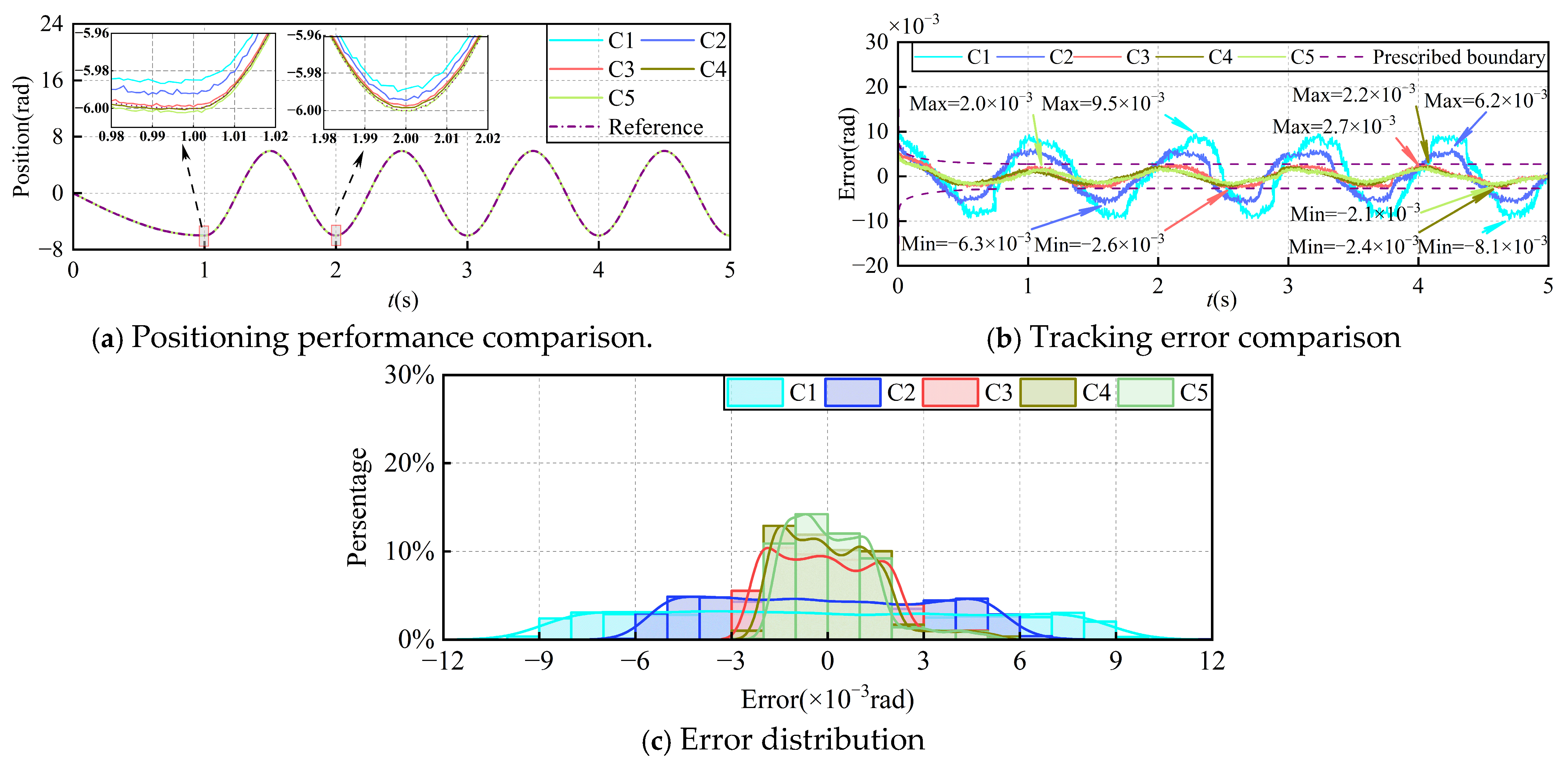
To verify the proposed controller’s ability to suppress time-varying disturbances, a sine wave signal with a varying period and an amplitude of 6 rad is given, along with a 0.2sin(2πt) N·m sine load disturbance. The tracking results under five control methods are shown in Figure 9 and Table 7. As seen in Figure 9 and Table 7, due to the time-varying nature of the applied load, the maximum error of the C1 and C2 methods increases by 0.0046 rad and 0.0024 rad, respectively, while the tracking error of the C3 method shows no significant change. The tracking error of the C4 and C5 methods converges within the preset boundary, and the overall tracking error stabilizes within a range of 0.003 rad. The maximum tracking error for the C5 method is 0.0021 rad, which is a reduction of 28.6% and 14.2% compared to C3 and C4 methods, respectively. The standard deviation of the tracking error for the C5 method is 2.52 rad, which is a reduction of 26.2% and 14.3% compared to C3 and C4 methods, respectively. The comparison shows that, when subjected to time-varying load disturbances, the controller proposed in this paper can better suppress disturbances and accurately track the desired trajectory, demonstrating stronger disturbance-suppression and recovery capabilities.

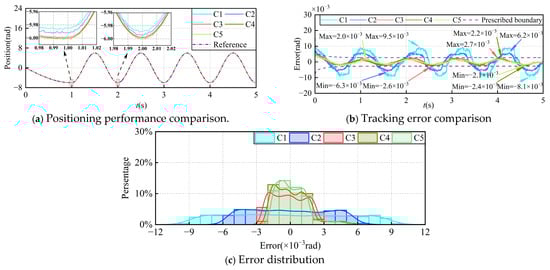
Figure 9. Operation result of sine position command under 0.2sin(2πt) N·m sine load disturbance.

Table 7. Tracking error performance metrics of sine position command under 0.2sin(2πt) N·m sine load disturbance.

Methods	eave (Rad)	emax (Rad)	estd (Rad)
C1	0.00041	0.0095	10.4
C2	0.00033	0.0063	6.7
C3	0.00024	0.0027	5.3
C4	0.00013	0.0024	4.8
C5	0.00013	0.0021	4.2

4.3.5. Experiment 5

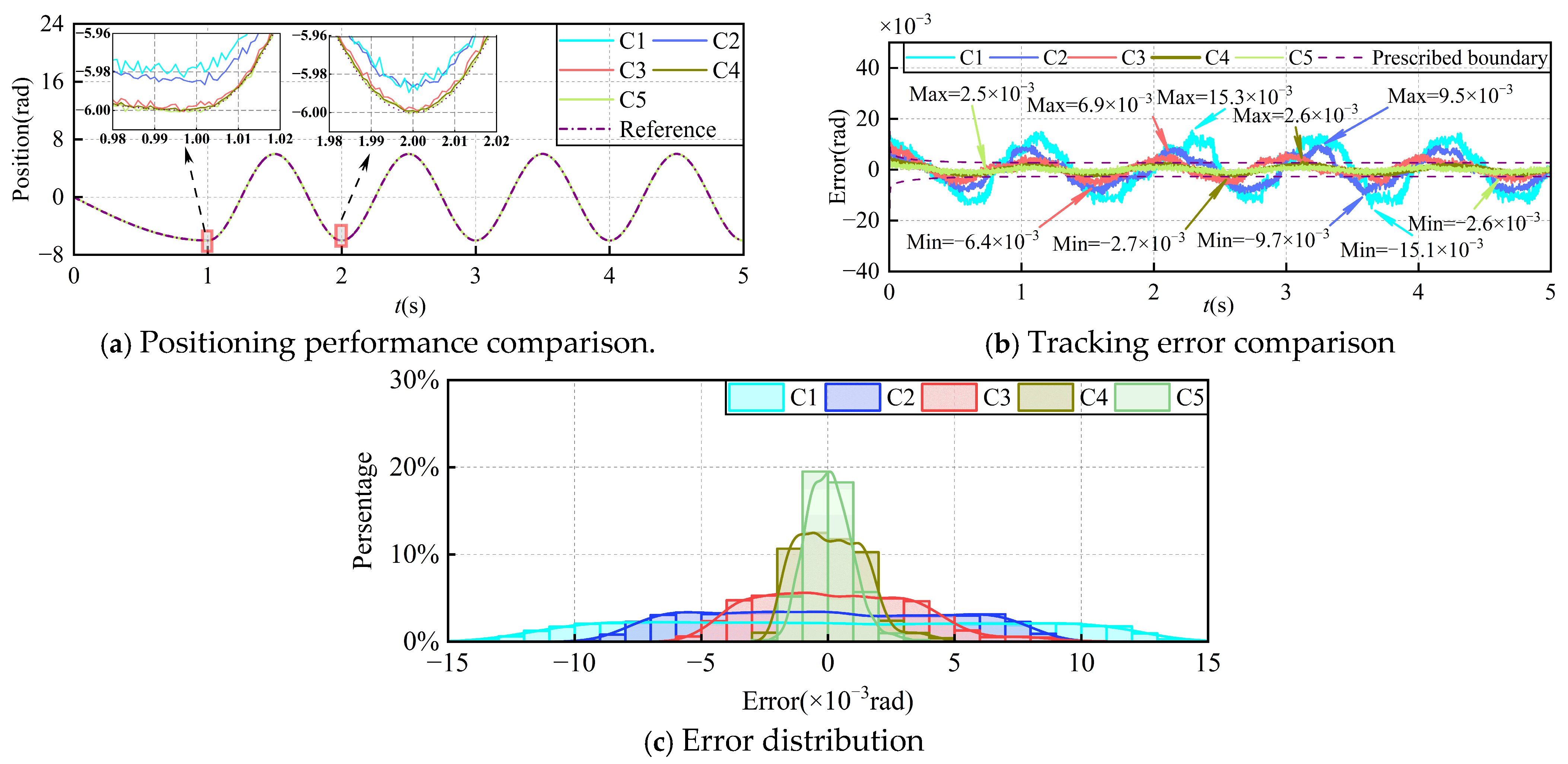
To verify the proposed controller’s ability to suppress disturbances in the presence of measurement noise, a sinusoidal wave signal with a variable period and amplitude of 6 rad is given, along with a 0.2sin(2πt) N·m sine load disturbance. The measurement noise is modeled as m(k) = 0.15(rand(1) − 0.5). The tracking results for five different control methods are shown in Figure 10 and Table 8. As seen in Figure 10 and Table 8, due to the time-varying characteristics of the applied measurement noise and load disturbances, the maximum errors for the C1 and C2 methods increase by 0.0104 rad and 0.0058 rad, respectively. The tracking error for the C3 method also shows a noticeable change. However, the C4 and C5 methods’ tracking errors converge within the preset boundary, with the overall tracking error remaining stable within a range of 0.003 rad. The maximum tracking error for the C5 method is 0.0026 rad, which is reduced by 3.84% and 165.4% compared to the C3 and C4 methods, respectively. The tracking error standard deviation for the C5 method is 1.7 rad, which is reduced by 58.8% and 141.1% compared to the C3 and C4 methods, respectively. Through the comparison, it can be concluded that, when subjected to measurement noise and a constant load, the proposed method offers a more satisfactory transition and tracking performance, with strong robustness against external disturbances.

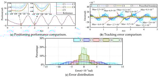
Figure 10. Operation result of sine position command under 0.2sin(2πt) N·m sine load disturbance and 0.15(rand(1) − 0.5) measurement noise.

Table 8. Tracking error performance metrics for sine position command under 0.2sin(2πt) N·m sine load disturbance and 0.15(rand(1) − 0.5) measurement noise.

Methods	eave (Rad)	emax (Rad)	estd (Rad)
C1	0.0074	0.0153	14.2
C2	0.0040	0.0097	9.4
C3	0.0030	0.0069	4.1
C4	0.0018	0.0027	2.7
C5	0.0010	0.0026	1.7

5. Conclusions

To enhance the position control accuracy of PMSMs, this paper proposes the PP-MFA-FITSMC method, which combines MFAC, DSGESO, and PP-FITSMC.

(1) In the MFAC framework, the proposed controller design does not rely on the mathematical model parameters of the PMSM, and DSGESO is utilized to observe and compensate for system states and disturbances, thus improving system robustness. By designing PP-FITSMC, the method further integrates the advantages of the improved prescribed performance function and FITSMC. This ensures that the position error converges within the prescribed bounds while retaining the fast response of the designed sliding mode surface and its disturbance rejection capability. The method is easy to implement and demonstrates strong practical control performance.

(2) To better understand the impact of controller parameter variations on system performance, a sensitivity analysis experiment for key controller parameters was designed using the response surface methodology. This yielded second-order regression equations relating the key parameters to the system settling time and steady-state error range. Based on the regression equations, the individual and interactive effects of these parameters on the control performance were quantified, providing valuable guidance for controller parameter tuning.

(3) Experimental comparisons show that PP-MFA-FITSMC outperforms other methods with faster convergence and no overshoot. In the presence of load disturbances and measurement noise, the tracking error of PP-MFA-FITSMC remains largely confined within ±0.001 rad, while the tracking errors of the other methods are more dispersed. This indicates that the proposed method effectively improves both the dynamic and steady-state performance and robustness of the PMSM position servo system.

Future work will focus on applying the proposed method to real-world engineering applications, providing further validation and enhancing the success rate of practical operations.

References

- Cheng, B.; Pang, S.Z.; Ou, H.Y.; Hu, Z.; Mao, Z.Y. Comparative Research on Topologies of Contra-Rotating Motors for Underwater Vehicles. J. Mar. Sci. Eng. 2023, 11, 2042. [Google Scholar] [CrossRef]
- Hidalgo, H.; Orosco, R.; Huerta, H.; Vazquez, N.; Estrada, L.; Pinto, S.; de Castro, A. A Finite-Set Integral Sliding Modes Predictive Control for a Permanent Magnet Synchronous Motor Drive System. World Electr. Veh. J. 2024, 15, 277. [Google Scholar] [CrossRef]
- Ma, C.; Huang, B.; Basher, M.K.; Rob, M.A.; Jiang, Y. Fuzzy PID Control Design of Mining Electric Locomotive Based on Permanent Magnet Synchronous Motor. Electronics 2024, 13, 1855. [Google Scholar] [CrossRef]
- Yao, R. Online d-q Axis Inductance Identification for IPMSMs Using FEA-Driven CNN. Ain Shams Eng. J. 2024, 15, 103130. [Google Scholar] [CrossRef]
- Jiang, W.; Han, W.; Wang, L.; Liu, Z.; Du, W. Linear Golden Section Speed Adaptive Control of Permanent Magnet Synchronous Motor Based on Model Design. Processes 2022, 10, 1010. [Google Scholar] [CrossRef]
- Wang, Y.; Liu, X. Model Predictive Position Control of Permanent Magnet Synchronous Motor Servo System with Sliding Mode Observer. Asian J. Control 2023, 25, 443–461. [Google Scholar] [CrossRef]
- He, C.; Hu, J.; Li, Y. Predictive Position Control with System Constraints for PMSM Drives Based on Geometric Optimization. IEEE Trans. Ind. Electron. 2023, 70, 7773–7782. [Google Scholar] [CrossRef]
- Gil, J.; You, S.; Lee, Y.; Kim, W. Nonlinear Sliding Mode Controller Using Disturbance Observer for Permanent Magnet Synchronous Motors under Disturbance. Expert. Syst. Appl. 2023, 214, 119085. [Google Scholar] [CrossRef]
- Wang, Y.; Liu, Y.; Ding, J.; Wang, D. Adaptive Type-2 Fuzzy Output Feedback Control Using Nonlinear Observers for Permanent Magnet Synchronous Motor Servo Systems. Eng. Appl. Artif. Intell. 2024, 131, 107833. [Google Scholar] [CrossRef]
- Hu, J.; He, C.; Li, Y. A Novel Predictive Position Control with Current and Speed Limits for PMSM Drives Based on Weighting Factors Elimination. IEEE Trans. Ind. Electron. 2022, 69, 12458–12468. [Google Scholar] [CrossRef]
- Gil, J.; You, S.; Lee, Y.; Kim, W. Super Twisting-Based Nonlinear Gain Sliding Mode Controller for Position Control of Permanent-Magnet Synchronous Motors. IEEE Access 2021, 9, 142060–142070. [Google Scholar] [CrossRef]
- Xu, J.; Xu, F.; Wang, Y.; Sui, Z. An Improved Model-Free Adaptive Nonlinear Control and Its Automatic Application. Appl. Sci. 2023, 13, 9145. [Google Scholar] [CrossRef]
- Li, X.; Ren, C.; Ma, S.; Zhu, X. Compensated Model-Free Adaptive Tracking Control Scheme for Autonomous Underwater Vehicles via Extended State Observer. Ocean. Eng. 2020, 217, 107976. [Google Scholar] [CrossRef]
- Chang, L.; Hou, Z. Two Description Encoding-Based Model-Free Adaptive Sliding Mode Control for Multiple-Input and Multiple-Output Nonlinear Systems. Nonlinear Dyn. 2025, 113, 10023–10042. [Google Scholar] [CrossRef]
- Zhang, W.; Xu, D.; Jiang, B.; Shi, P. Virtual-Sensor-Based Model-Free Adaptive Fault-Tolerant Constrained Control for Discrete-Time Nonlinear Systems. IEEE Trans. Circuits Syst. I Regul. Pap. 2022, 69, 4191–4202. [Google Scholar] [CrossRef]
- Corradini, M.L. A Robust Sliding-Mode Based Data-Driven Model-Free Adaptive Controller. IEEE Control Syst. Lett. 2022, 6, 421–427. [Google Scholar] [CrossRef]
- Gu, C.; Tan, C.; Li, B.; Lu, J.; Wang, G.; Chi, X. Data-Driven Model-Free Adaptive Sliding Mode Control for Electromagnetic Linear Actuator. J. Micromech. Microeng. 2022, 32, 055007. [Google Scholar] [CrossRef]
- Li, J.; Tang, Y.; Zhao, H.; Wang, J.; Lu, Y.; Dou, R. Under-Actuated Motion Control of Haidou-1 ARV Using Data-Driven, Model-Free Adaptive Sliding Mode Control Method. Sensors 2024, 24, 3592. [Google Scholar] [CrossRef]
- Wei, X.; Sui, Z.; Peng, H.; Xu, F.; Xu, J.; Wang, Y. Model-Free Adaptive Sliding Mode Control Scheme Based on DESO and Its Automation Application. Processes 2024, 12, 1950. [Google Scholar] [CrossRef]
- Liu, Y.; Liu, X.P.; Jing, Y.W.; Zhou, S.W. Adaptive Backstepping H∞ Tracking Control with Prescribed Performance for Internet Congestion. ISA Trans. 2018, 72, 92–99. [Google Scholar] [CrossRef]
- Jing, C.; Xu, H.; Niu, X. Adaptive Sliding Mode Disturbance Rejection Control with Prescribed Performance for Robotic Manipulators. ISA Trans. 2019, 91, 41–51. [Google Scholar] [CrossRef] [PubMed]
- Esmaeili, B.; Salim, M.; Baradarannia, M. Predefined Performance-Based Model-Free Adaptive Fractional-Order Fast Terminal Sliding-Mode Control of MIMO Nonlinear Systems. ISA Trans. 2022, 131, 108–123. [Google Scholar] [CrossRef] [PubMed]
- Huang, X.; Dong, Z.; Zhang, F.; Zhang, L. Discrete-time Extended State Observer-based Model-free Adaptive Sliding Mode Control with Prescribed Performance. Int. J. Robust. Nonlinear Control 2022, 32, 4816–4842. [Google Scholar] [CrossRef]
- Huang, X.; Dong, Z.; Zhang, F.; Zhang, L. Model-free Adaptive Integral Sliding Mode Constrained Control with Modified Prescribed Performance. IET Control Theory Appl. 2023, 17, 1044–1060. [Google Scholar] [CrossRef]
- Zou, Q.; Sun, L.; Chen, D.; Wang, K. Adaptive Sliding Mode Based Position Tracking Control for PMSM Drive System with Desired Nonlinear Friction Compensation. IEEE Access 2020, 8, 166150–166163. [Google Scholar] [CrossRef]
- Xu, Y.; Wu, A. Integral Sliding Mode Predictive Control with Disturbance Attenuation for Discrete-time Systems. IET Control Theory Appl. 2022, 16, 1751–1766. [Google Scholar] [CrossRef]
- Gao, W.; Wang, Y.; Homaifa, A. Discrete-Time Variable Structure Control Systems. IEEE Trans. Ind. Electron. 1995, 42, 117–122. [Google Scholar]
- Kim, D.; Rhee, S. Design of an Optimal Fuzzy Logic Controller Using Response Surface Methodology. IEEE Trans. Fuzzy Syst. 2001, 9, 404–412. [Google Scholar]
- Camcıoğlu, Ş.; Özyurt, B.; Doğan, İ.C.; Hapoğlu, H. Application of Response Surface Methodology as a New PID Tuning Method in an Electrocoagulation Process Control Case. Water Sci. Technol. 2017, 76, 3410–3427. [Google Scholar] [CrossRef]
Disclaimer/Publisher’s Note: The statements, opinions and data contained in all publications are solely those of the individual author(s) and contributor(s) and not of MDPI and/or the editor(s). MDPI and/or the editor(s) disclaim responsibility for any injury to people or property resulting from any ideas, methods, instructions or products referred to in the content. |
© 2025 by the authors. Published by MDPI on behalf of the World Electric Vehicle Association. Licensee MDPI, Basel, Switzerland. This article is an open access article distributed under the terms and conditions of the Creative Commons Attribution (CC BY) license (https://creativecommons.org/licenses/by/4.0/).