Article

Path Tracking of Autonomous Vehicle Based on Optimal Control

1
School of Intelligent Manufacturing, Weifang Institute of Technology, Weifang 261000, China
2
School of Machinery and Automation, Weifang University, Weifang 261061, China
*
Author to whom correspondence should be addressed.
World Electr. Veh. J. 2025, 16(7), 340; https://doi.org/10.3390/wevj16070340
Submission received: 18 April 2025 / Revised: 17 June 2025 / Accepted: 18 June 2025 / Published: 20 June 2025

Abstract

:
Path tracking control is a key technology in the research of intelligent vehicles. In the path tracking process of intelligent vehicles, there are multiple constraints and time-varying nonlinear system states. To address the problems of low tracking accuracy and poor robustness, a method based on Radau pseudospectral method(RPM) is designed. Firstly, a 4-DOF vehicle model was established. Secondly, the multiple phase Radau pseudospectral method(MPRPM) was used to discretize the control and state variables. Then, the path tracking problem was transformed into a nonlinear programming problem. Finally, the method was compared with other control methods such as Gaussian pseudospectral method(GPM) and linear quadratic regulator (LQR). The simulation results show that the tracking error of the proposed method is 0.075 m while those of the GPM and LQR are 0.029 m and 0.05 m, respectively. The simulation and virtual as well as the real vehicle test results indicate that the method can control the vehicle track the given path while meeting various constraint requirements achieving ideal results and good tracking accuracy.

1. Introduction

Nowadays, autonomous driving can improve urban traffic efficiency and reduce traffic emissions. It is a key technology for the construction of intelligent transportation and smart cities. The high precision of vehicle path tracking control is one of the cores of autonomous driving and the foundation of intelligent vehicle operation. Research on control strategies for autonomous driving of vehicles aiming to ensure that the actual driving route of intelligent vehicles coincides with the target path as much as possible can reduce the lateral position deviation and heading angle deviation of the actual driving path relative to the target path and thus ensure the accuracy of intelligent vehicle path tracking control. The key technologies of autonomous vehicles include environmental perception, decision-making, motion planning, and tracking control. Currently, issues such as path tracking, lane keeping, and vehicle lane changing have become hot research issues in the field of intelligent connected vehicles. And research on path tracking has received widespread attention. It mainly reduces the distance and direction deviation between vehicles and target paths during path tracking through appropriate control algorithms, thereby achieving the goal of improving path tracking accuracy. Vehicle path tracking is a highly nonlinear optimization problem that is strictly constrained by various constraints (control constraints, state constraints and terminal constraints). It is research based on the original trajectory design, aiming to re-optimize one or more objective characteristics and multi-task requirements to obtain the optimal performance value that satisfies numerous constraint conditions. Optimization not only saves costs, but also has certain guiding significance for achieving higher performance indicators under the same cost conditions. Therefore, in various complex environments, designing a trajectory design and optimization method to quickly generate an optimal trajectory that satisfies multiple constraints is a problem of great theoretical significance and engineering value, which is also one of the hot issue of research in the past decade, especially at present at home and abroad [1,2,3].
Stanley control is a feedback based nonlinear control method with few parameters and easily to be designed [4]. The design process of backstepping control is simple and has high control accuracy. However, as the system order increases, hyperparameters may occur. Yu et al. and Yin et al. proposed a nonlinear robust control method for underactuated systems with unmatched uncertainty. This method could handle system uncertainty and has good robustness [5,6]. Sliding mode control system has strong anti-interference ability and fast response speed, and is a highly reliable and effective control method. Its unique design enables the system to stably control the target variable in complex environments without being affected by external interference [7]. Imine et al. developed a sliding mode controller based on the super twist algorithm which was mainly used to accurately control the lateral deviation and yaw angle deviation of the vehicle, thereby effectively tracking the target path [8]. Han et al. proposed a new arrival law with dynamic coefficients and a trajectory tracking method based on sliding mode control which accelerated the response speed of the controller [9]. Sabiha et al. considered the factors of vehicle slip in actual operating conditions [10]. At the same time, some classic adaptive control methods were provided for solving the path tracking problem [11,12,13,14].
Reference [15] firstly selected appropriate initial values and then uses the collocation point method to solve the trajectory optimization problem under complex constraint conditions during vehicle driving, finding its local optimal solution. Reference [16] summarized the domestic and international research on trajectory optimization algorithms in recent years, and elaborated in detail on the basic principles of various pseudospectral methods represented by different coordinate polynomials. It also summarized the advantages and disadvantages of various methods in trajectory optimization design applications. Reference [17] addressed various issues in the process of vehicle path tracking, including strong coupling, strong nonlinearity, and parameter uncertainty. Reference [18] was based on the traditional pseudospectral method and incorporated a feedback system to obtain a rolling optimization closed-loop tracking scheme, which solved the problem of vehicle path tracking under multiple constraint conditions. It calculated and provided state feedback based on online real-time trajectory optimization algorithms to achieve real-time instruction updates. Benson et al. proposed the Gauss pseudospectral method, and its prominent contribution was the proof of the Gaussian pseudospectral covariate mapping theorem. The difference between the GPM and other pseudospectral methods lies in the dynamic pseudospectral method. The state constraint was not configured at the boundary point, and this configuration, along with a set of approximate covariate variables, formed a Karush Kuhn Tucker (KKT) condition that was consistent with the discretization form of the first-order optimal necessary condition at the LG point. Benson provided a detailed argument on the equivalence between this KKT condition and the first-order necessary condition of discretization, which enabled nonlinear programming (NLP) solutions to satisfy the first-order optimality necessary condition of traditional indirect methods and avoided the drawbacks of general direct methods [19]. Huntington and Rao studied the trajectory optimization problem of spacecraft formation flight based on GPM. The optimization objective was to determine the minimum transfer of the spacecraft formation from the parking orbit to the reference orbit with minimal fuel consumption. The optimization results demonstrated the applicability of GPM in formation flight. In addition, they proposed an improved solution to the GPM for solving optimal control problems, applying Pontryagin’s minimum principle to boundary points, which was more effective at the starting and ending points. In boundary control optimization, applying initial state variables and covariate variables could achieve higher accuracy. Compared with using extrapolation to control boundary conditions, it significantly improved the accuracy of optimizing trajectories and could be applied in real-time optimization control [20]. DivyaGarg et al. applied the GPM to the nonlinear infinite domain optimal control problem and proved the KKT condition and a solution to the discrete infinite domain optimal control problem. The optimality condition had consistency, and applying KKT multiplier vector mapping could accurately obtain the covariate variables [21]. Mei et al. studied the fuel optimal control problem of satellite relative orbit transfer in elliptical orbit based on the Legendre pseudospectral method. A performance index matching the true near point angle was given for the satellite relative motion dynamics model with the true near point angle as the independent variable. The Legendre pseudospectral method was used to transform the optimal control problem into a parameter optimization problem. Based on the state transition matrix, an optimal control law with only the initial and final states as constraints was given. For the linearized model, an optimal control law constrained by the state equation was proposed. The Legendre pseudospectral method was widely used in aircraft trajectory optimization due to its high efficiency and real-time computing capability. It was one of the earliest and most widely studied pseudospectral methods, but further improvement was needed in terms of computational accuracy [22].
The adaptive Radau pseudospectral method can provide high-precision approximate solutions when solving multiple order differential equations and can ensure that the vehicle accurately tracks the preset trajectory. Meanwhile, the adaptive Radau pseudospectral method is more efficient in handling complex boundary conditions. It can effectively handle the complex constraints and generate continuous and practically feasible trajectories. At the same time, it can transform continuous time optimal control problems into discrete nonlinear programming problems, thereby simplifying the calculation process. When constructing differential matrices, for the adaptive Radau pseudospectral method, the differential matrix is sparse, effectively reducing storage and computational complexity, and has certain advantages in solving vehicle path tracking problems.
The Radau pseudospectral method itself can provide high-precision approximate solutions, and the multi-interval Radau pseudospectral method divides the entire solution interval into multiple sub-intervals, which can more accurately approximate the true solution on each sub-interval. When solving the problem of vehicle trajectory tracking, it can accurately approximate the state and control variables of the vehicle on each subinterval, thereby improving the overall trajectory tracking accuracy. Therefore, the paper uses the adaptive RPM to solve the problem that satisfies multiple constraints. In the rest of the paper: Section 2 presents the mathematical Model. Section 3 provides the adaptive pseudospectral method. Section 4 presents the numerical simulation and experimental verification. Section 5 presents the conclusions of the paper.

2. Vehicle Model

2.1. Mathematical Model of Vehicle

A nonlinear 4-DOF vehicle model shown in Figure 1.
In the state space form, it is [1]:
v ˙ = u ω + F y f cos δ + F y r + F x f sin δ m ω ˙ r = a F y f cos δ b F y r + a F x f sin δ I z u ˙ = v ω + F x f cos δ F y f sin δ + F x r F f F w m δ ˙ = p p ˙ = k 1 ξ 1 I w u v k 1 ξ 1 a I w u ω + ( k 1 ξ 1 k w ) I w δ c w I w p + T s w i I w
The state is x ( t ) = [ u ( t ) , v ( t ) , ω ( t ) , x ( t ) , y ( t ) ] and the control is z ( t ) = [ δ ] . Then Equation (2) can be obtained.
x ˙ = f [ x ( t ) , z ( t ) ]

2.2. Optimal Control Object

The cost function is [1]:
J ( z ) = t 0 t f y y d E ^ 2 + z T ^ s w 2 dt = t 0 t f L ( x , z ) dt

2.3. Constraints

(1) The initial and terminal states are described as
x ( t 0 ) = [ u ( t 0 )   ,   0   ,   0 ,   0 , 0   ] T
x ( t f ) = [ u ( t f )   ,   0   ,   0 ,   x ( t f )   ,   y ( t f )   ] T
(2) When the vehicle is driven by front wheel drive,
F x f μ m g b a + b + μ h g F x r = 0
where μ is the road friction coefficient; h g is the height vehicle center of mass.
F x f and F x r should be met:
F x f μ m g ( b + μ h g ) a + b F x r = a μ h g b + μ h g F x f
(3) Control and state variable constraints
Z ( t ) l Z ( t ) Z ( t ) h
where Z ( t ) h and Z ( t ) l are the upper and lower bounds of the steering angle. The steering wheel angle is controlled in −600–600°.
So, the optimal path tracking problem is
min J ;   s . t .   x ˙ = f [ x ( t ) ,   u ( t ) , t ] ,   h 0
where h 0 expresses the inequality constraint.
The optimal vehicle path tracking problem in this article can be described as an optimal control problem within a finite time. That is, within the time interval t [ t 0 , t f ] and based on the given state variable x ( t ) R n , the control variable z ( t ) R m is determined so that the vehicle tracks from the initial state x ( t 0 ) to the terminal state x ( t f ) under the constraint conditions, and the specified performance indicator is optimal.
min   J = Φ ( x ( t 0 ) , t 0 , x ( t f ) , t f ) + t 0 t f L ( x ( t ) , z ( t ) , t ) dt
s . t . x ˙ ( t ) = f ( x ( t ) , z ( t ) , t ; t 0 , t f ) C ( x ( t ) , z ( t ) , t ; t 0 , t f ) 0 φ ( x ( t 0 ) , t 0 , x ( t f ) , t f ) = 0  

3. Adaptive Pseudospectral Method

3.1. Multiple Phase Adaptive Radau Pseudospectral Method

Firstly, the time interval t [ t 0 , t f ] of the optimal control problem is divided into K subintervals and each sub-interval S k = [ t k 1 , t k ] , k = 1 , 2 , 3 , , K is transformed into the interval τ [ 1 , 1 ] using Equation (12).
τ = 2 t t k t k 1 t k t k 1
Due to the fact that the Radau pseudospectral method uses the Legendre–Gauss–Radau (LGR) collocation points, it is necessary to generate LGR collocation points using Legendre polynomial P N ( τ ) which is defined as
P N ( τ ) = 1 2 N N ! d N d τ N [ ( τ 2 1 ) N ]
Each collocation point is the root of the polynomial P N 1 ( τ ) + P N ( τ ) = 0 . Therefore, the corresponding collocation point on the time interval τ [ 1 , 1 ] can be obtained for each group interval through Equation (13).
On the interval S k = [ t k 1 , t k ] , N k LGR collocation points and τ N k + 1 = 1 are set as interpolation nodes. The optimal control problem is discretized in each subinterval using generated N k + 1 node. In the interval S k , k [ 1 , 2 , 3 , , K ] , the state variables can be approximated as [23,24]:
x ( k ) ( τ ) X ( k ) ( τ ) = j = 1 N K + 1 X j ( k ) L X , j ( k ) ( τ )
where X ( k ) ( τ ) is a N k order approximate polynomial. L j ( k ) ( τ ) is a set of Lagrange polynomials which are expressed as [25,26]:
L X , j ( k ) ( τ ) = l = 1 , l j N k + 1 τ τ l ( k ) τ j ( k ) τ l ( k )
x ˙ X ˙ = j = 1 N K + 1 X j L ˙ j = j = 1 N K + 1 X j D i j , ( i = 1 , 2 , , N k )
where D i j = L ˙ j ( t i ) is an N k × ( N k + 1 ) matrix which is called the Radau pseudospectral differential matrix.
And the discrete form is
u ( k ) ( τ ) U ( k ) ( τ ) = j = 1 N K U j ( k ) L U , j ( k ) ( τ )
L U , j ( k ) ( τ ) = l = 1 , l j N k τ τ l ( k ) τ j ( k ) τ l ( k )
In summary, the optimal control problem for continuous time can be discretized into a NLP problem of algebraic form, namely:
min J = Φ ( X 1 ( 1 ) , t 0 , X N K + 1 ( K ) , t f ) + k = 1 K i = 1 N k t f t 0 2 ω i ( k ) L X i ( k ) , Z i ( k ) , τ i ( k ) ; t 0 , t f
where ω i ( k ) is the weight:
ω 1 ( k ) = 2 N k ω i ( k ) = 1 ( 1 τ i ( k ) ) [ P N k 1 ( τ i ( k ) ) ] 2   i = 1 , 2 , , N k
This type of problem can be solved using mature optimization algorithm tools.

3.2. Adaptive Collocation Point Method

The estimated values X τ ^ 1 ( k ) , , X τ ^ M k ( k ) of the state variables corresponding to these nodes can be obtained from Equation (14).
Another state variable estimation of integral form can be obtained by utilizing M k nodes:
X ^ ( k ) ( τ ^ j ( k ) ) = X ( k ) ( τ k 1 ) + t f t 0 2 l = 1 M k I ^ j l ( k ) f X ( k ) ( τ ^ l ( k ) ) , U ( k ) ( τ ^ l ( k ) ) , τ ^ l ( k ) ) j = 2 , , M K + 1
where I ^ ( k ) is an M k × M k LGR integration matrix.
E i ( k ) ( τ ^ l ( k ) ) = X ^ i ( k ) ( τ ^ l ( k ) ) X i ( k ) ( τ ^ l ( k ) )
e i ( k ) ( τ ^ l ( k ) ) = E i ( k ) ( τ ^ l ( k ) ) 1 + max j [ 1 , , M k + 1 ] X i ( k ) ( τ ^ l ( k ) ) l 1 , , M k + 1 ; i = 1 , , n y
So, S k can be defined as
e max ( k ) = max i 1 , , n y l 1 , , M k + 1 e i ( k ) ( τ ^ l ( k ) )
If e max ( k ) is greater than ε , nodes can be added:
P k = log N k e max ( k ) ε
If P k is not an integer:
N ˜ k = P k + N k
If N ˜ k N max B k
B k = max N ˜ k N min , 2
where N min is the set minimum order. If B k is not an integer, then it is rounded up.
In summary, the adaptive strategy adopted in this article firstly increases the order of the polynomial within the interval. When the order reaches the maximum required order, the subinterval is further divided to achieve subdivision of the interval and improve accuracy.

3.3. Calculation Process of Multi-Interval Radau Pseudospectral Method

  • Step (1). Dividing the entire time into K subintervals, each subinterval being S k = [ t k 1 , t k ] , k = 1 , 2 , 3 , , K .
  • Step (2). Transforming the optimal control problem into an NLP problem using LGR collocation points for solution.
  • Step (3). Calculating e max ( k ) for each subinterval using Equation (19). If e max ( k ) ε , the available result is obtained; otherwise, proceeding to Step (4).
  • Step (4). Using Equation (20) to increase the order of the polynomial within each sub-interval; using Equation (21) to update the number of collocation points and interval numbers within each subinterval.
  • Step (5). Repeating step (2).

4. Result Analysis

4.1. Numerical Simulations

In the simulation, ε is set as 10−4; N min is set as 5; N max is set as 15.
For the simulations, the calculation parameters are shown in Table 1.
The co-simulation flow chart is shown in Figure 2.

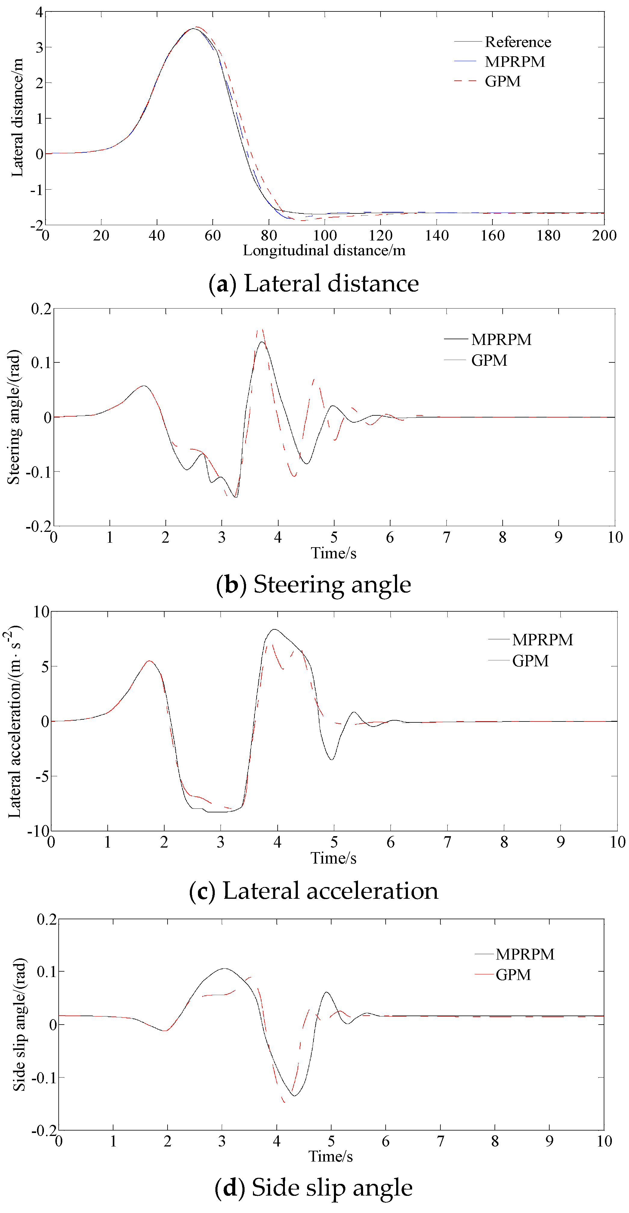
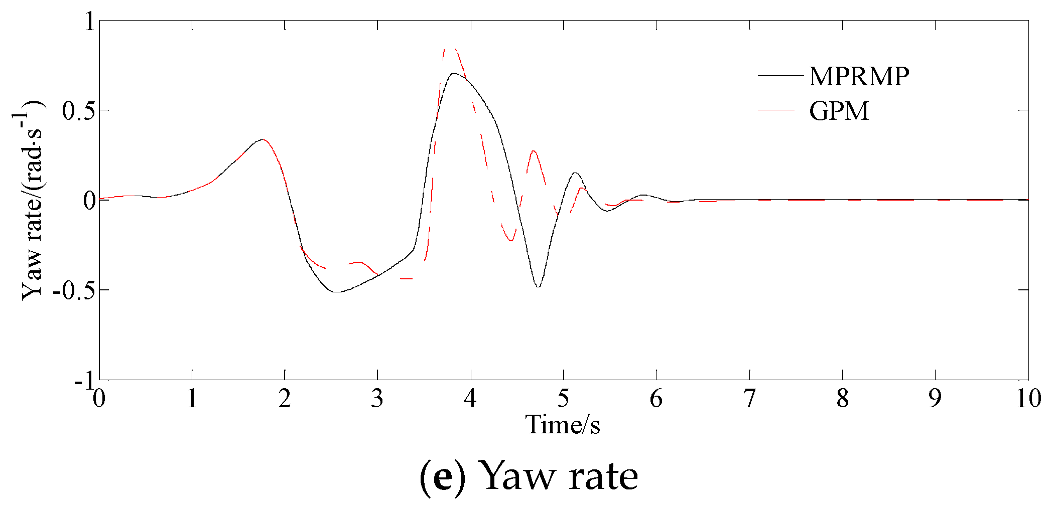
4.1.1. Double Lane Changing Road

The road adhesion coefficient is set as 0.85 and the vehicle velocity is selected as 20 m/s.
Figure 3a shows that the two control methods can effectively track the given path well under the condition of double lane changing road.
As shown in Figure 3b, due to the small curvature of the road curve at the turn, the steering angle of the vehicle exhibits peak values. At the same time, the peak values of the steering angle controlled by the proposed method are relatively small, indicating that the vehicle controlled by this method can easily and accurately track the given path.
Figure 3c indicates that the proposed method can use bigger lateral acceleration to complete the process of path tracking with minimum time than other traditional methods.
From Figure 3d, it can be seen that the method proposed in this paper has better control effects on the side slip angle indicating the better lateral stability of the vehicle and better driving stability.
Figure 3e shows that the method improves the control accuracy, significantly reduces yaw rate, enables the vehicle to better track the given path, reduces unstable driving conditions and improves the real-time and accurate response of intelligent vehicles to driving commands.

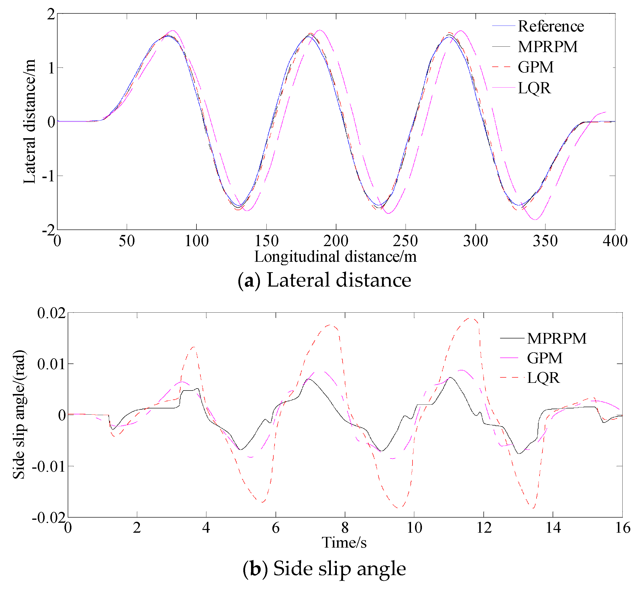
4.1.2. Serpentine Road

As depicted in Figure 4a, the lateral offset of the three methods demonstrate a high degree of proximity to the reference values in this scenario. However, due to the low adhesion coefficient, the LQR method has a certain degree of lag in the responses of lateral distance.
As depicted in Figure 4b, the MPRPM continues to exhibit the most effective stability control, ensuring that the amplitude of the side slip angle does not exceed 0.0076 rad. However, the maximum value of the side slip angle of the GPM and LQR are 0.01 rad and 0.18 rad. The maximum yaw rate of controller II are 0.0091 rad and 0.155 rad/s, respectively, indicating the stability control performance of the MPRPM.
As depicted in Figure 4c, the yaw rate of the GPM and LQR method are 0.165 rad/s and 0.175 rad/s, respectively. However, the yaw rate of the MPRPM is just 0.15 0.165 rad/s.

4.2. Analysis of Control Performance

In Figure 5, the comparison curve of the MPRPM and GPM as well as LQR it shows that, on the basis of the pseudospectral method, the hp adaptive Radau pseudospectral method can converge faster while ensuring high accuracy and optimality of the optimized solution which significantly improves the path tracking performance and handling stability of the entire vehicle, thereby greatly enhancing active safety. The mean of absolute error of lateral distance of the MPRPMs is 0.075 m while those of the GPM and LQR are 0.029 m and 0.05 m, respectively. The control method can ensure the stability of vehicle operation.

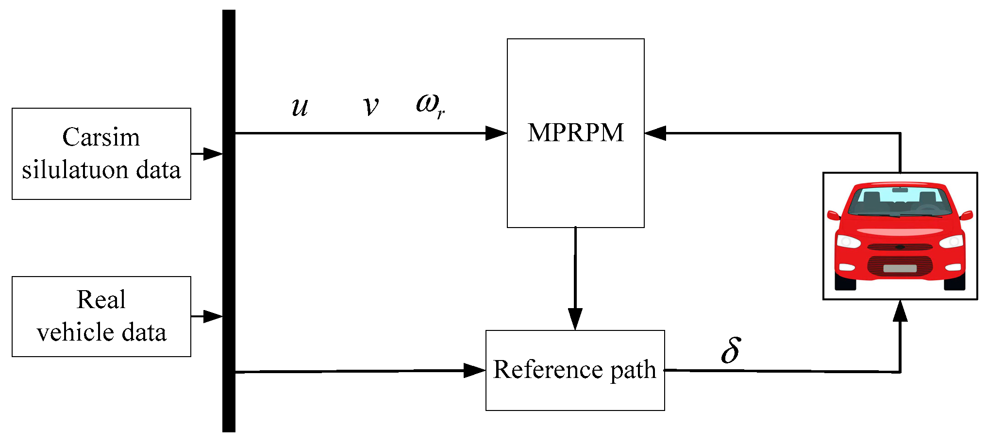
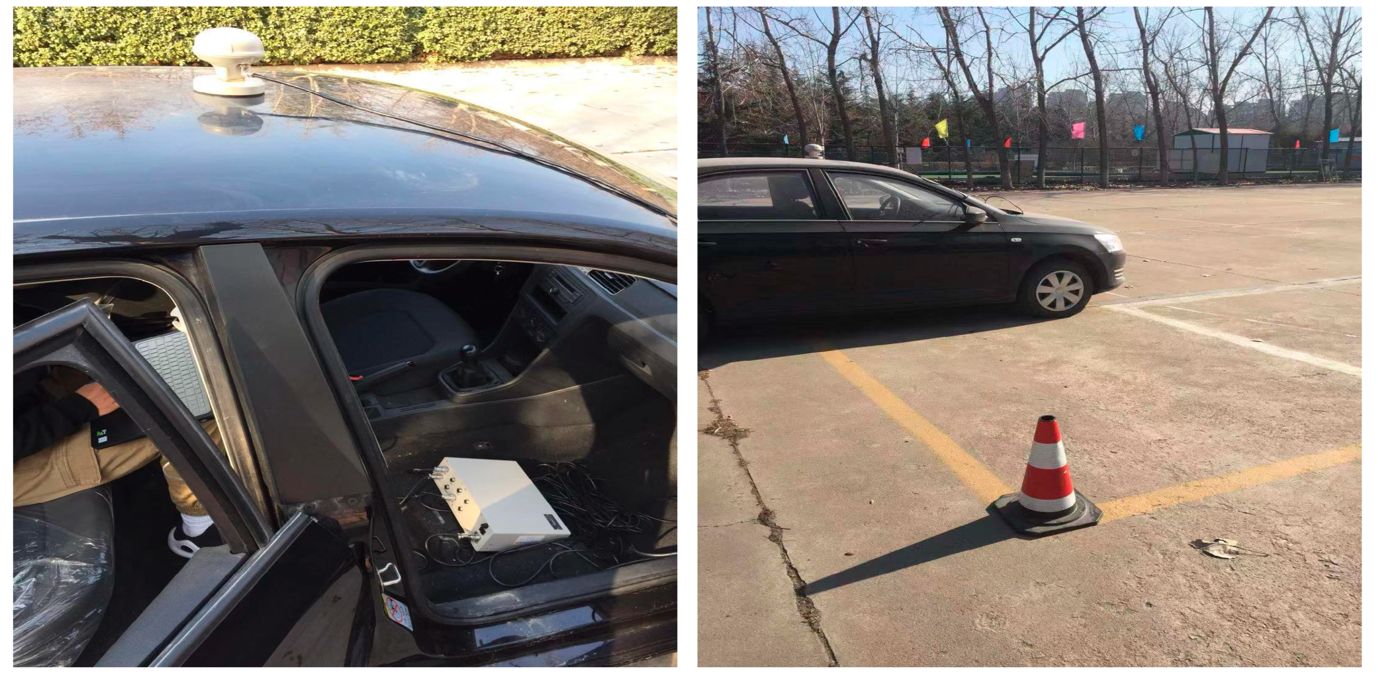
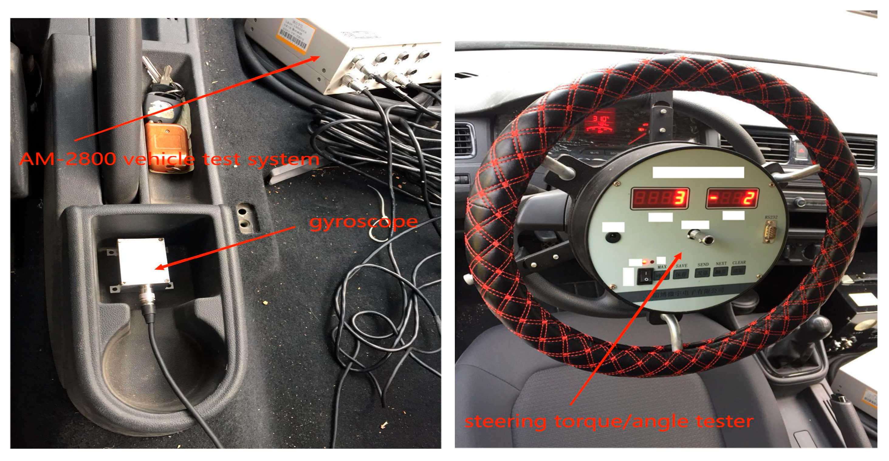
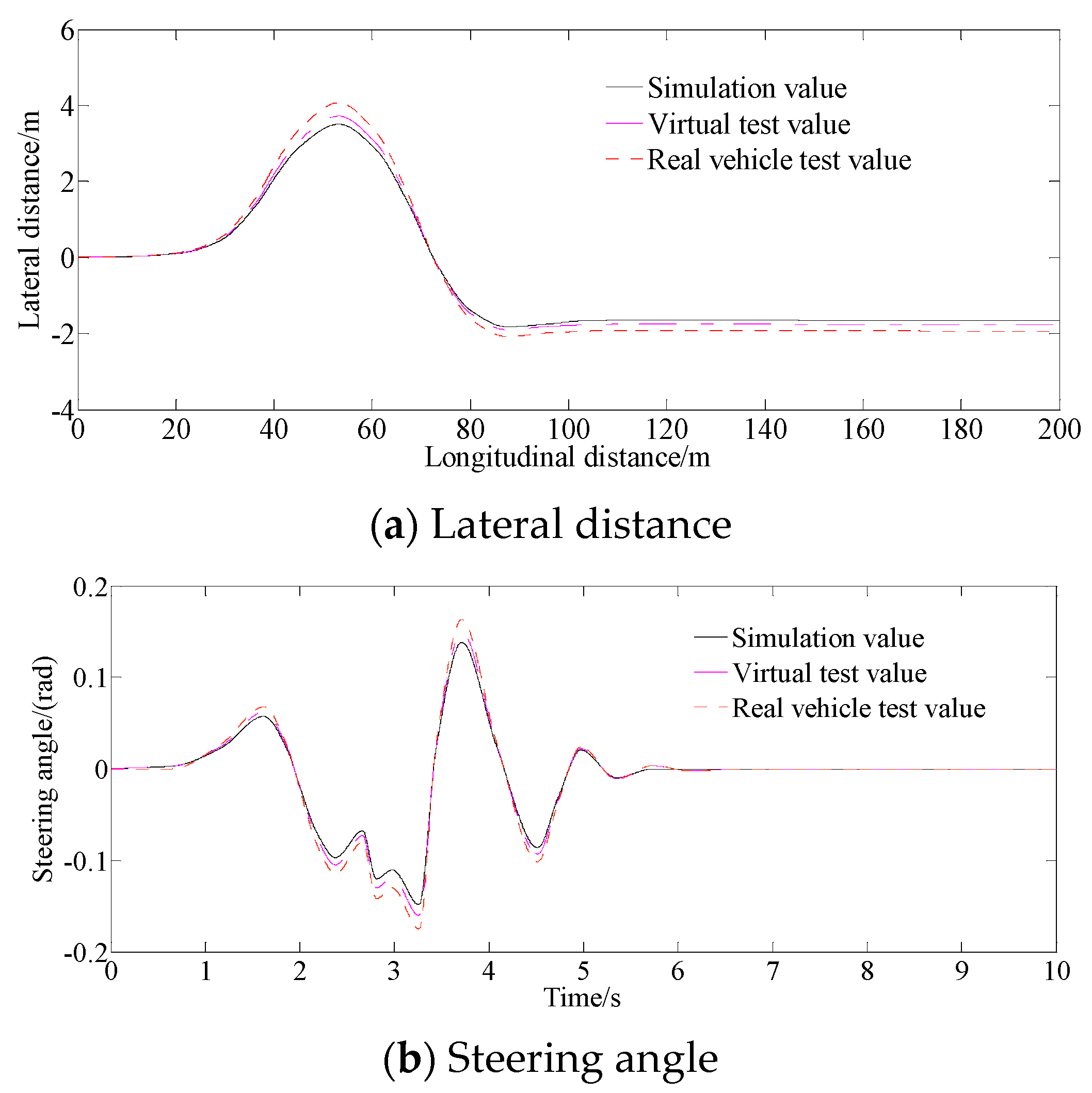
4.3. Experimental Verification

Carsim software (2019) can customize various vehicle models such as small cars, SUVs, etc., as well as customize road alignment index parameters. It can intuitively observe the three-dimensional animation and related indicators of the vehicle driving process, obtain parameter values that reflect the stability, smoothness, and other related indicators of the vehicle driving, establish the relationship between the vehicle mechanical characteristics and road operation safety. The Carsim simulation method can simplify, visualize, and quantify the complex operational status of vehicles. The Carsim work interface consists of three main parts: Model Parameters and Inputs, Run Control, and Output and Post Processing. The software development team uses symbolic multi-body programs in Vehicle Sim Lisp to generate mathematical model equations for vehicles. In addition to providing accurate solutions to highly complex nonlinear equation systems, the model equations have also been highly optimized for rapid computation. The processing speed of the Carsim model is usually more than ten times faster than the running speed of a personal computer with a frequency of 3 GHz, so results can be obtained quickly. Carsim supports real-time testing and hardware in the loop (HIL) systems. High processing speed is also beneficial for software’s repeated calculations such as optimization, design, and experimentation. Carsim packages almost all the tools required by users to predict vehicle dynamic characteristics into one, and can collaborate with other software to further expand its functionality. Carsim combines decades of precision in simulation model research with the ease of software use.
The real experimental vehicle is shown in Figure 6. The measurement devices are shown in Figure 7.
The experimental results are shown in Figure 8.
In Figure 8a, the maximum error between the virtual test and simulation values is 0.15 m. However, the maximum error between the real vehicle test and simulation values is 0.3 m. In Figure 8b the maximum error between the real vehicle test and simulation values is bigger than the one between the virtual test and simulation values, which is caused by the response lag of the control steering actuator and the driving skills of the driver.
The virtual and real vehicle test verification results of the double lane changing road show that both the trends of lateral distance and steering angle of the curve are consistent.

4.4. Summary of Different Path Tracking Methods

In this section, based on the above analysis, the advantages and disadvantages of different path tracking methods are summarized. The summary is shown in Table 2.

5. Conclusions

This paper investigates the problem of vehicle path tracking using the multiple phase Radau pseudospectral method. In order to verify the actual effectiveness of the control method designed in this article, a comparative verification of double lane changing simulation is conducted. The proposed method was compared with traditional control methods of GPM and LQR methods. The proposed method is 0.075 m while those of the GPM and LQR are 0.029 m and 0.05 m, respectively. The vehicle can complete path tracking process in the shortest time while meeting various constraint requirements. The method proposed in this article can provide some reference for the design of path tracking control for unmanned vehicles. Although multi-interval partitioning reduces the computational complexity of each subinterval to a certain extent, an increase in the number of subintervals will lead to an overall increase in computational complexity. Especially when the sub-intervals are divided very finely, operations such as point selection, weight calculation, and differential matrix construction need to be performed on each sub-interval, which significantly increases the computation time. In the future, the real-time performance of the algorithm needs in-depth research.

Author Contributions

Methodology, Y.L.; Software, B.W.; Data curation, Y.L.; Writing-original draft, Y.L.; Writing—review & editing, Q.W. All authors have read and agreed to the published version of the manuscript.

Funding

This research was supported by the Open Research Program of Huzhou Key Laboratory of Urban Multidimensional Perception and Intelligent Computing under Grant No. UMPIC202404. The authors gratefully acknowledge the support agency.

Institutional Review Board Statement

Not applicable.

Informed Consent Statement

Not applicable.

Data Availability Statement

The related data used to support the findings of this study are available from the corresponding author upon request.

Conflicts of Interest

The authors declare no conflicts of interest.

Nomenclature

RPMRadau pseudospectral method;
MPRPMmultiple phase Radau pseudospectral method;
GPMGaussian pseudospectral method;
LQRlinear quadratic regulator;
KKTKarush Kuhn Tucker;
NLPnonlinear programming;
LGRLegendre–Gauss–Radau;
m (kg)vehicle mass;
Iz (kg∙m2)moment of inertia around the z axis;
a (m)distances of front axle from the center of gravity;
b (m)distances of rear axle from the center of gravity;
k1 (N∙rad−1)synthesized stiffness of front tire;
k2 (N∙rad−1)synthesized stiffness of rear tire;
itransmission ratio of the steering system;
Iw (kg·m2)moment of inertia of the steering system;
c w / ( N · m · s · rad 1 ) drag coefficient;
k w / ( N · m · rad 1 ) synthesized cornering stiffness;
ξ 1 / m front wheel aligning arm of force;
hg (m)height of the center gravity.

References

  1. Liu, Y.J.; Cui, D.W.; Peng, W. Optimum Control for Path Tracking Problem of Vehicle Handling Inverse Dynamics. Sensors 2023, 23, 6673. [Google Scholar] [CrossRef]
  2. Liu, Y.J.; Cui, D.W. Estimation algorithm for vehicle state estimation using ant lion optimization algorithm. Adv. Mech. Eng. 2022, 14, 16878132221085839. [Google Scholar] [CrossRef]
  3. Liu, Y.J.; Cui, D.W.; Peng, W. Optimal Lane Changing Problem of Vehicle Handling Inverse Dynamics Based on Mesh Refinement Method. IEEE Access 2023, 11, 115617–115626. [Google Scholar] [CrossRef]
  4. Hwang, C.L.; Yang, C.C.; Hung, J.Y. Path tracking of an autonomous ground vehicle with different payloads by hierarchical improved fuzzy dynamic sliding-mode control. IEEE Trans. Fuzzy Syst. 2018, 26, 899–914. [Google Scholar] [CrossRef]
  5. Yu, R.; Ding, S.; Tian, H.; Chen, Y.H. A hierarchical constraint approach for dynamic modeling and trajectory tracking control of a mobile robot. J. Vib. Control. 2022, 28, 564–576. [Google Scholar] [CrossRef]
  6. Yin, H.; Chen, Y.H.; Huang, J.; Lü, H. Tackling mismatched uncertainty in robust constraint-following control of underactuated systems. Inf. Sci. 2020, 520, 337–352. [Google Scholar] [CrossRef]
  7. Wu, Y.; Wang, L.; Zhang, J.; Li, F. Path following control of autonomous ground vehicle based on nonsingular terminal sliding mode and active disturbance rejection control. IEEE Trans. Veh. Technol. 2019, 68, 6379–6390. [Google Scholar] [CrossRef]
  8. Imine, H.; Madani, T. Sliding-mode control for automated lane guidance of heavy vehicle. Int. J. Robust Nonlinear Control. 2013, 23, 67–76. [Google Scholar] [CrossRef]
  9. Han, Y.X.; Cheng, Y.; Xu, G.W. Trajectory tracking control of AGV based on sliding mode control with the improved reaching law. IEEE Access 2019, 7, 20748–20755. [Google Scholar] [CrossRef]
  10. Sabiha, A.D.; Kamel, M.A.; Said, E.; Hussein, W.M. ROS-based trajectory tracking control for autonomous tracked vehicle using optimized backstepping and sliding mode control. Robot. Auton. Syst. 2022, 152, 104058. [Google Scholar] [CrossRef]
  11. Zhang, S.W.; Ma, L.; Li, Q.; Wang, H. Observer-based adaptive path tracking control for autonomous ground vehicle with singularities and time-varying delays. J. Mech. Sci. Technol. 2025, 39, 1443–1456. [Google Scholar] [CrossRef]
  12. Dekhterman, S.R.; Norris, W.R.; Nottage, D.; Soylemezoglu, A. Hierarchical Rule-Base Reduction Fuzzy Control for Path Tracking Variable Linear Speed Differential Steer Vehicles. IEEE Trans. Fuzzy Syst. 2025, 33, 828–841. [Google Scholar] [CrossRef]
  13. Zhou, X.; Wang, H.; Li, Q.; Wu, L. Adaptive path tracking control for autonomous vehicles with sideslip effects and unknown input delays. Trans. Inst. Meas. Control. 2025, 47, 444–453. [Google Scholar] [CrossRef]
  14. Zhang, S.; Wang, Y.; Li, G.; Wang, Y. Path tracking control of autonomous vehicles via prescribed performance approach. Neural Comput. Appl. 2025, 37, 3839–3856. [Google Scholar] [CrossRef]
  15. Xu, D.H.; Xu, G.J.; Ye, S.X.; Wu, X.F.; Tang, D.J. Nonlinear Closed-loop Optimal Ascent Guidance for Aerospace Vehicle Based on Pseudospectral Method. Tactical Missile Technol. 2017, 4, 57–65. [Google Scholar]
  16. Hu, S.Q.; Chen, Y. Analysis of pseudospectral methods applied to aircraft trajectory optimization. J. Rocket. Propuls. 2014, 40, 61–68. [Google Scholar]
  17. Liu, Y.J.; Cui, D.W. Optimal Control of Vehicle Path Tracking Problem. World Electr. Veh. J. 2024, 15, 429. [Google Scholar] [CrossRef]
  18. Chen, T.T.; Sun, C.Z. Flight Corridor Planning Method of RBCC Ascent. Ordnance Ind. Autom. 2019, 38, 50–53. [Google Scholar]
  19. Benson, D. A Gauss Pseudospectral Transcription for Optimal Control. Ph.D. Thesis, Massachusetts Institute of Technology, Cambridge, MA, USA, 2004. [Google Scholar]
  20. Huntington, G.T.; Rao, A.V. Optimal reconfiguration of spacecraft formation using the Gauss pseudospectral method. AIAA J. Guid. Control. Dyn. 2008, 31, 689–698. [Google Scholar] [CrossRef]
  21. Garg, D.; William, W.H.; Rao, A.V. Gauss pseudospectral method for solving infinite-horizon optimal control problems. In Proceedings of the AIAA Guidance Navigation Control Conference, AIAA, Toronto, ON, Canada, 2–5 August 2010; pp. 1011–1020. [Google Scholar]
  22. Mei, J.; Ma, G.F.; Yang, B. Fuel-optimal control of satellite relative orbit transfer based on legendre pseudospectral method. J. Harbin Inst. Technol. 2010, 42, 352–357. [Google Scholar]
  23. Betts, J.T. Practical methods for optimal control and estimation using nonlinear programming. Appl. Mech. Rev. 2002, 55, 1–449. [Google Scholar] [CrossRef]
  24. Yan, C.X.; Tong, Y.A.; Song, J.H.; Lu, B.G.; Zhao, L.B. Optimization of Trajectory with Terminal Constraints Based on Multiple Phase Radau Pseudospectral Method. Tactical Missile Technol. 2021, 2, 94–100. [Google Scholar]
  25. Geoffrey, T.; Huntington; Rao, A.V. Optimal Configuration of Spacecraft Formations Via A Gauss Pseudospectral Method. Adv. Astronaut. Sci. 2005, 120, 33–50. [Google Scholar]
  26. Benson, D.A.; Huntington, G.T.; Thorvaldsen, T.P.; Rao, A.V. Direct Trajectory Optimization and Costate Estimation via an Orthogonal Collocation Method. J. Guid. Control. Dyn. 2006, 29, 1435–1440. [Google Scholar] [CrossRef]
Figure 1. 4-DOF vehicle model.
Wevj 16 00340 g001
Figure 2. Flow chart of co-simulation.
Wevj 16 00340 g002
Figure 3. Simulation result of double lane changing road.
Wevj 16 00340 g003aWevj 16 00340 g003b
Figure 4. Simulation result of serpentine road.
Wevj 16 00340 g004aWevj 16 00340 g004b
Figure 5. Comparison results between MPRPM, GPM and LQR.
Wevj 16 00340 g005
Figure 6. Real test vehicle.
Wevj 16 00340 g006
Figure 7. Measurement devices.
Wevj 16 00340 g007
Figure 8. Experimental results.
Wevj 16 00340 g008
Table 1. Simulation parameters.
ParameterValue
m (kg)1265
Iz (kg·m2)1800
a (m)1.170
b (m)1.195
k1 (N·rad−1)60,042
k2 (N·rad−1)109,295
i20
Iw (kg·m2)16.38
c w / ( N · m · s · rad 1 ) 140
k w / ( N · m · rad 1 ) 0
ξ 1 / m 0.021
hg (m)0.53
Table 2. Summary of path tracking methods.
AlgorithmsMean of Absolute Error of Path Tracking(m)AdvantagesDisadvantages
MPRPM0.075The MPRPM utilizes Gauss integration to configure differential algebraic equations at discrete points, resulting in higher computational efficiency. Meanwhile, the MPRPM exhibits good convergence.For large-scale or multi- interval problems, the MPRPM may require significant computational resources and time, especially when performing high-precision calculations.
GPM0.029The GPM has the characteristics of high computational accuracy, good stability, and wide applicability. When dealing with complex constraint conditions, GPM remains efficient and can generate smooth and constraint compliant paths.In some cases, GPM may be sensitive to initial conditions. And improper selection of initial conditions may lead to convergence problems or suboptimal solutions.
LQR0.05LQR can obtain the optimal control law of state linear feedback, which makes it easy to form closed-loop optimal control, thereby achieving system stability and performance optimization.The performance of LQR is highly sensitive to the selection of weight matrices Q and R, and improper parameter selection may lead to system performance degradation or instability.
Disclaimer/Publisher’s Note: The statements, opinions and data contained in all publications are solely those of the individual author(s) and contributor(s) and not of MDPI and/or the editor(s). MDPI and/or the editor(s) disclaim responsibility for any injury to people or property resulting from any ideas, methods, instructions or products referred to in the content.

