Emission/Reliability-Aware Stochastic Optimization of Electric Bus Parking Lots and Renewable Energy Sources in Distribution Network: A Fuzzy Multi-Objective Framework Considering Forecasted Data

Abstract

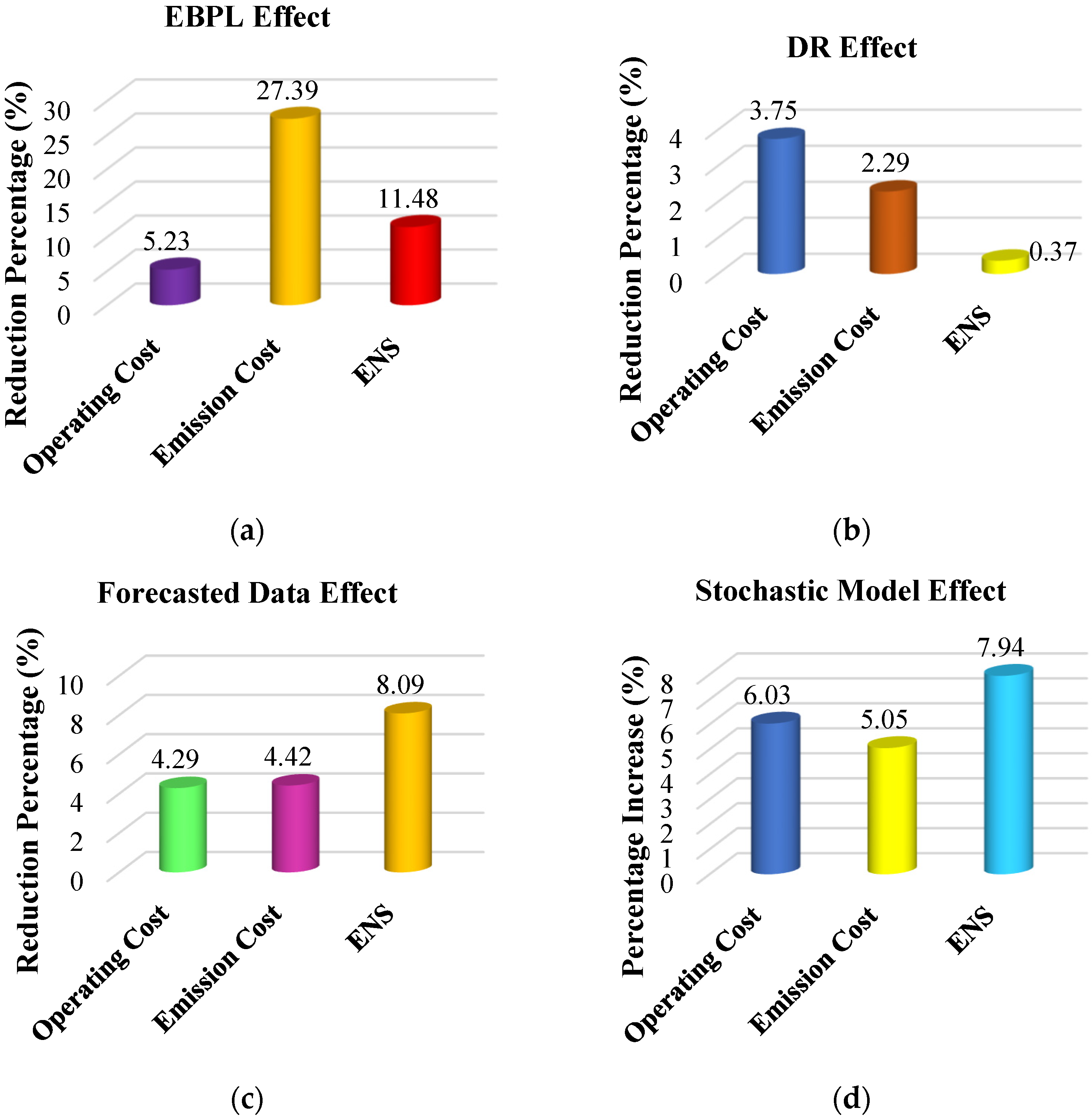
In this paper, an emission- and reliability-aware stochastic optimization model is proposed for the economic planning of electric bus parking lots (EBPLs) with photovoltaic (PV) and wind-turbine (WT) resources in an 85-bus radial distribution network. The model simultaneously minimizes operating, emission, and energy-loss costs while increasing system reliability, measured by energy not supplied (ENS), and uses a fuzzy decision-making approach to determine the final solution. To address optimization challenges, a new multi-objective entropy-guided Sinh–Cosh Optimizer (MO-ESCHO) is proposed to efficiently mitigate premature convergence and produce a well-distributed Pareto front. Also, a hybrid forecasting architecture that combines MO-ESCHO and artificial neural networks (ANN) is proposed for accurate prediction of PV and WT power and network loading. The framework is tested across five cases, progressively incorporating EBPL, demand response (DR), forecast information, and stochastic simulation of uncertainties using a new hybrid Unscented Transformation–Cubature Quadrature Rule (UT-CQR) method. Comparative analyses against conventional methods confirm superior performance in achieving better objective values and ensuring computational efficiency. The outcomes indicate that the combination of EBPL with RES reduces operating costs by 5.23%, emission costs by 27.39%, and ENS by 11.48% compared with the base case with RES alone. Moreover, incorporating the stochastic model increases operating costs by 6.03%, emission costs by 5.05%, and ENS by 7.94% over the deterministic forecast case, reflecting the added complexity of uncertainty. The main contributions lie in coupling EBPLs and RES under uncertainty and proposing UT-CQR, which exhibits robust system performance with reduced variance and lower computational effort compared with Monte Carlo and cloud-model approaches.

1. Introduction

Transport electrification has emerged as a central pillar of global efforts to curb greenhouse gas emissions and enable a sustainable energy transition [1]. Although light-duty electric vehicles (EVs) have led research and deployment in recent years, focus has increasingly turned toward public transit and heavy-duty fleets, with electric buses (EBs) being in the spotlight [1]. In comparison with dispersed individual EVs and their highly variable user behavior, EBs take fixed routes and schedules and have their charging requirements far more predictable and controllable [2,3]. Grid-to-Bus (G2B) refers to the charging mode in which electric buses receive energy from the grid, while Bus-to-Grid (B2G) denotes the discharging mode in which stored energy from electric buses is supplied back to the grid to support demand and improve system stability. Such an operation enables the integration of electric bus parking lots (EBPLs) into power grids not only as large loads but also as controllable, flexible energy resources [4]. EBPLs outperform scattered EVs in several ways. Their central charging points are amenable to coordinated control, making it possible for system operators to reduce peak demand, offer ancillary services, and improve overall stability. Their scheduled charging patterns are more predictable and easier to plan for than the uncertainty associated with non-public EV charging. EBPLs can also be utilized as distributed energy storage, absorbing excess energy and feeding it back to the grid, thereby assisting in network balancing. The combination of EBPLs with RES, such as PV panels and WTs, further increases these advantages [5]. Distribution networks, which would otherwise rely heavily on upstream grid purchases, can reduce costs and emissions by using local RES generation [6]. Local generation also reduces network losses by serving demand closer to the point of consumption. EBPLs supplement this plan by storing excess RES and injecting it during peak demand periods to reduce energy not supplied (ENS) and improve operational reliability. Combined, EBPLs and RES minimize operating costs, decrease the cost of emissions, and enhance the distribution system’s efficiency. Even with these benefits, the combined usage of EBPLs and RES introduces substantial uncertainties. Uncertainties induced by randomness in solar irradiance, wind speed, and load demand lead to stochastic outputs. Conventional deterministic optimization methods, which ignore uncertainty, tend to underestimate risk and may yield suboptimal or infeasible solutions. It is for this reason that stochastic optimization models are needed to capture the probabilistic behavior of RES generation and demand fluctuations [7]. Therefore, system operators can identify solutions that are not only sustainable and cost-effective but also robust and resilient under real operating conditions.

The integration of RES and electric parking lots (EPLs) into distribution networks has been an area of intense research interest in recent years. These resources can reduce power losses, improve voltage profiles, and provide increased system reliability. The following section reviews major studies proposing optimization solutions in this context. In [8], the authors formulated an optimal placement strategy for EVs, PV panels, and WTs in distribution systems using an MILP model. Environmental aspects, along with the uncertainties in load demand and renewable generation, were considered. Its primary objective was to minimize the discounted investment and operating costs while ensuring stable and sustainable system performance over the planning horizon. In [9], a framework was presented to balance the participation of EVs and RES in distribution networks. The framework aimed to maximize financial returns for market participants using an intelligent control strategy for EV charging and discharging. The proposed market-oriented EV management system was tested on a real distribution grid and then explored to assess its impact on network operation, particularly with respect to voltage control and system stability. The work in [10] investigated the optimal siting and sizing of EV charging and hydrogen fueling stations supplied by a hybrid renewable power system configuration of wind, solar, and battery storage. The optimization minimized the annualized construction, maintenance, and operating costs under stochastic demand, energy-price variability, and renewable-generation uncertainty. The study contributes to sustainable urban energy–infrastructure planning through the combined planning of alternative energy transport terminals. In [11], a coordinated day-ahead scheduling framework was presented for EVs in collaboration with renewable generators to participate in energy and reserve markets. The optimization was framed to achieve economic efficiency relative to system constraints. Large-scale computational simulations verified the performance of the scheduling scheme and demonstrated expanded market participation. However, this paper, and a couple of earlier ones, did not rigorously explore the potential adverse effects of such coordination on the hosting distribution grid. The paper in [12] introduced an innovative concept of a smart distribution grid hosting a virtual power plant (VPP), within a framework of Coupled Virtual Entities (CVEs). These entities were modeled to trade simultaneously in energy and reactive-power markets so as to maximize profits under stochastic market prices, load variations, and random renewable generation. The strategy highlighted the versatility of CVEs in ancillary services provision, grid-voltage stability, and economic benefits. A multi-objective model for distribution-system reconfiguration with Vehicle-to-Grid (V2G)-equipped EVs and renewable sources was presented in [13]. The objectives entailed minimizing power losses, minimizing voltage deviations, and increasing the voltage-stability index through strategic control of EV charging and discharging operations. In this study, the operational advantages of transactive-control approaches were demonstrated for grid resilience and energy efficiency. The framework suggested in [14] established a two-tier transactive-energy market enabling decentralized energy trading among EV charging stations with on-site solar PV arrays. Using a game-theoretic approach, charging points engaged in local energy exchanges while a top-level market operated by the distribution system operator (DSO) coordinated them. The model illustrated how distributed decision-making can improve competition and system-wide efficiency while respecting network limitations. In [15], various approaches to synchronizing EV operation with renewable generation were examined from a techno-economic perspective. The research concluded that smart charging is more cost-effective in the short term, whereas V2G operation is advantageous in the long term due to enhanced use of EV battery storage capacity. The investigation provided valuable insights into trade-offs between economic efficiency and operational flexibility in EV–RES coordination. A comprehensive integration analysis of a photovoltaic (PV) plant and an electric-vehicle parking lot was presented in [16]. The research compared impacts on power load, energy losses, and grid dependence under different operating conditions. The proposed parking facility operates with both grid supply and rooftop solar PV generation, offering a green alternative with reduced peak load and enhanced system dependability.

The integration of RES and electric parking lots (EPLs) into distribution networks has been an area of intense research interest in recent years. These resources can reduce power losses, improve voltage profiles, and provide increased system reliability. The following section reviews major studies proposing optimization solutions in this context. In [8], the authors formulated an optimal placement strategy for EVs, PV panels, and WTs in distribution systems using an MILP model. Environmental aspects, along with uncertainties in load demand and renewable generation, were considered. Its primary objective was to minimize discounted investment and operating costs while ensuring stable and sustainable system performance over the planning horizon. In [9], a framework was presented to balance the participation of EVs and RES in distribution networks. The framework aimed to maximize financial returns for market participants using an intelligent control strategy for EV charging and discharging. The proposed market-oriented EV management system was tested on a real distribution grid and then explored to assess its impact on network operation, particularly with respect to voltage control and system stability. The work in [10] investigated the optimal siting and sizing of EV-charging and hydrogen-fueling stations supplied by a hybrid renewable power system configuration of wind, solar, and battery storage. The optimization minimized the annualized construction, maintenance, and operating costs under stochastic demand, energy-price variability, and renewable-generation uncertainty. The study contributes to sustainable urban energy–infrastructure planning through the combined planning of alternative energy transport terminals. In [11], a coordinated day-ahead scheduling framework was presented for EVs in collaboration with renewable generators to participate in energy and reserve markets. The optimization was framed to achieve economic efficiency relative to system constraints. Large-scale computational simulations verified the performance of the scheduling scheme and demonstrated expanded market participation. However, this paper, and a couple of earlier ones, did not rigorously explore the potential adverse effects of such coordination on the hosting distribution grid. The paper in [12] introduced an innovative concept of a smart distribution grid hosting a virtual power plant (VPP), within a framework of Coupled Virtual Entities (CVEs). These entities were modeled to trade simultaneously in energy and reactive-power markets so as to maximize profits under stochastic market prices, load variations, and random renewable generation. The strategy highlighted the versatility of CVEs in ancillary-services provision, grid-voltage stability, and economic benefits. A multi-objective model for distribution-system reconfiguration with Vehicle-to-Grid (V2G)-equipped EVs and renewable sources was presented in [13]. The objectives entailed minimizing power losses and voltage deviations and increasing the voltage-stability index through strategic control of EV charging and discharging operations. In this study, the operational advantages of transactive-control approaches were demonstrated for grid resilience and energy efficiency. The framework suggested in [14] established a two-tier transactive-energy market enabling decentralized energy trading among EV charging stations with on-site solar PV arrays. Using a game-theoretic approach, charging points engaged in local energy exchanges while a top-level market operated by the distribution system operator (DSO) coordinated them. The model illustrated how distributed decision-making can improve competition and system-wide efficiency while respecting network limitations. In [15], various approaches to synchronizing EV operation with renewable generation were examined from a techno-economic perspective. The research concluded that smart charging is more cost-effective in the short term, whereas V2G operation is advantageous in the long term due to enhanced use of EV battery storage capacity. The investigation provided valuable insights into trade-offs between economic efficiency and operational flexibility in EV–RES coordination. A comprehensive integration analysis of a PV plant and an electric-vehicle parking lot was presented in [16]. The research compared impacts on power load, energy losses, and grid dependence under different operating conditions. The proposed parking facility operates with both grid supply and rooftop solar PV generation, offering a green alternative with reduced peak load and enhanced system dependability.

In [17], an optimization model was proposed to maximize the utilization of EV charging infrastructure in power systems that also accommodate renewable generation, such as solar resources. The strategy reduced operating expenses while allowing a smart system to predict vehicle arrival patterns and optimize charging behavior. The proposed framework demonstrated improved energy management and economic performance in smart-grid systems. Reference [18] introduced a voltage-management framework that synchronizes PV generation, EVs, conventional grid devices, and responsive loads. A mixed-integer nonlinear multi-objective optimization model was used with a Chebyshev goal-programming method to derive an optimal trade-off among multiple objectives, namely minimizing PV curtailment, system losses, and unmet demand, while flattening the voltage profile. The results underscored the importance of optimized synchronization in maintaining system stability. The planning model in [19] was directed toward designing an electric-vehicle charging ecosystem (EVCE) that involves distributed solar power generation and a distribution static compensator (DSTATCOM). The model assessed the long-term technical, economic, and environmental impacts of various planning options. Optimal siting and sizing of EVCE components were achieved with a particle swarm optimization (PSO) algorithm using a success-rate criterion. The study also included a detailed cost–benefit analysis covering installation, operation, and maintenance. The optimal design of a hybrid renewable system comprising PV, WT, and battery units for a grid-connected EV charging station based on V2G technology was considered in [20]. The authors employed a rule-based energy-management strategy (RB-EMS) to track power exchanges and incorporated a multi-objective enhanced arithmetic optimization algorithm (MOIAOA) to identify optimal component sizes. The optimization jointly minimized the levelized cost of electricity and grid dependence while maximizing energy export to the grid.

A two-step process was proposed in [21] for efficient EVCS and DG planning in distribution networks. In the first step, a fuzzy max–min approach with PSO was used to find the most cost-effective locations and capacities for EVCSs. The second step minimized the combined costs of EV users and the network operator while maximizing station profitability, taking into account EV waiting times and grid constraints. In [22], coordination of PV panels, wind turbines (WTs), and EV units in a radial distribution network was optimized to minimize power losses and improve voltage stability. The random nature of load demand was incorporated using a Multi-Population Evolution Whale Optimization Algorithm (MEWOA), which effectively handled conflicting parameters to optimize network performance. The concurrent location and capacity planning for refueling stations for electric vehicles supplied by hybrid renewable energy resources such as PV, WT, and bio-waste generation with energy storage was addressed in [23]. Optimization employed a bi-level framework that minimized annual operating and energy-loss costs while considering the interrelation between top-level planning and bottom-level operational decisions under a smart-grid network. In [24], a multi-objective expansion-planning model was proposed to decide EVCS siting and sizing and network reinforcement in high wind-energy-penetration networks. The optimization was performed to reduce overall investment and energy-loss costs while, simultaneously, maximizing captured traffic flow to enhance infrastructure utilization. Uncertainty in wind-power generation was treated explicitly to increase realism in the planning. A dynamic control strategy for EV charging/discharging to avoid overvoltage and reverse power-flow problems due to excessive PV generation in distribution systems was developed in [25]. By adaptive management of charging rates based on network conditions, the strategy provided improved voltage regulation and reduced reverse-power effects compared with conventional fixed-rate schemes. Ref. [26] proposed a probabilistic planning framework for long-term EV parking lot operation. By forecasting the probability of EV arrival at each facility, the proposed model maximized investor profit through an NSGA-based approach. This method enhanced allocation efficiency and avoided potential congestion in urban networks.

A summary of the literature is presented in Table 1.

Table 1. Summary of the literature.

Ref. No.	Device	Objective Function	Findings	Limitations
[8]	PV, WT, EV	Minimize investment and operational costs	Optimal allocation of RE and EV	Did not assess emission
[9]	EV, PV, WT	Maximize participant revenue via optimal EV charge/discharge	Enhanced system efficiency and voltage regulation	Focused mainly on market
[10]	PV, WT, Hydrogen, Battery	Minimize total annual cost	Cost-effective stochastic siting of EV and hydrogen stations	Did not exchange real-time operation with grid
[11]	PV, WT, EV	Minimize operational cost and participate in reserve markets	Economic efficiency and renewable utilization	Did not evaluate the grid hosting
[12]	PV, WT, EV	Maximize expected profits under market uncertainties	Flexible energy and reactive power participation	Limited reliability
[13]	PV, WT, EV (V2G)	Minimize power loss, voltage deviation; enhance voltage stability	Grid resilience and efficiency via V2G coordination	Did not include stochastic model
[14]	PV, EV	Enable energy trading among EVCSs with on-site PV	Efficiency enhancement	Ignored stochastic operation
[15]	PV, WT, EV	Evaluate techno-economic performance of EV-RE coordination strategies	Smart charging with V2G	No formal stochastic optimization
[16]	PV, EV	Minimize energy losses and grid dependency	Reliability enhancement	Did not incorporate stochastic optimization
[17]	PV, EV	Minimize operational cost; optimize EV behavior prediction	Intelligent management of EV charging	Focused on prediction, not stochastic planning
[18]	PV, EV, Responsive Loads	Minimize PV curtailment, system losses, unmet demand	Balanced trade-offs and stable voltage profile	Computationally heavy
[19]	PV, EV, DSTATCOM	Optimize site/capacity to minimize cost and emissions	Techno-economic assessment of EVCE integration	Did not examine operational stochastic model
[20]	PV, WT, Battery, EV	Optimize hybrid system sizing, minimize cost, maximize grid export	Hybrid RE-EVCS performance via V2G operation	Limited study on reliability impacts
[21]	EV, DG	Minimize user/network costs; maximize operator profit	Stochastic EVCS allocation	Did not consider emissions and reliability
[22]	PV, WT, EV	Reduce power loss, enhance voltage stability	Network performance under uncertain load	Did not analyze emission
[23]	PV, WT, Bio-waste, EV	Minimize annual operating and energy loss costs	Validated cost reduction	Complex coordination; lacks adaptability
[24]	WT, EV	Minimize total cost, energy losses; maximize traffic flow	Accounted for wind generation uncertainty	Did not study on emission
[25]	PV, EV	Mitigate overvoltage and reverse flow	Better voltage support and reduced reverse power flow	Focused on operational control
[26]	EV	Maximize profit via probabilistic EV arrival modeling	Enhanced allocation and reduced congestion	Did not include emission analysis
[27]	WT, EV, Battery	Minimize cost-to-revenue ratio under uncertainty	Reliable scheduling considering uncertainty	Did not explore emission and reliability

The following major gaps in research are synthesized from the literature:

• Insufficient focus on EBPL integration in distribution networks: Despite several studies [8,9,10,11,12,13,15,16,22,23] analyzing the integration of EVs with renewable energy sources, the majority focus on light-duty or dispersed EVs, with limited consideration for centralized electric bus parking lots (EBPLs). These have distinguishing characteristics due to their extensive storage capacity, controllability, and significant impact on network operation. There is a shortage of detailed studies on EBPL planning and operation under conditions of renewable abundance, which limits understanding of their impact on network reliability and cost-effectiveness.
• Inadequate treatment of uncertainty in renewable and load parameters: Despite stochastic considerations being partially addressed in some contributions [8,10,11,19,21,22,24], uncertainty is often handled using simplified or deterministic approaches, neglecting the true variability of solar, wind, and demand profiles. The majority of existing models apply fixed scenarios or probability distributions without considering temporal correlation or variability propagation. This gap highlights the need for a robust stochastic framework capable of addressing multiple sources of uncertainty simultaneously.
• Limitations of existing metaheuristic optimization techniques: Most works employ metaheuristic approaches such as PSO [19], MEWOA [22], NSGA-II [26], and other evolutionary algorithms [13,14,18], but these techniques are often affected by premature convergence, poor adaptability, and diminished exploration in high-dimensional, multi-objective environments. Few works have explored innovative or hybrid optimization techniques that dynamically trade off exploration and exploitation or maintain solution diversity to improve global search efficacy.
• Limited integration of forecasting within optimization frameworks: Though renewable forecasting is identified as crucial for system operation, few studies [17,20,25] integrate predictive information on renewable generation or load behavior directly. Nearly all existing works conduct optimization using static or past data, without accounting for the possible benefit of forecast-driven optimization. The absence of hybrid forecasting–optimization models limits the ability to minimize energy not supplied (ENS), emission levels, and operating costs based on real-world uncertainties.
• High computational burden of classical stochastic techniques: Previous work using conventional stochastic techniques such as Monte Carlo simulation (MCS) or cloud models [8,19,24] entails heavy computational effort and inconsistent outcomes due to the substantial number of samples required to ensure convergence. These limitations point to the need for computationally effective stochastic optimization models with high-quality, stable output at lower processing requirements without sacrificing reliability or robustness.

This paper introduces an emission- and reliability-aware stochastic optimization framework for the simultaneous planning of EBPLs and RES in distribution networks. The key contributions and novelties include:

• Combined Planning of EBPL and RES in Distribution Systems: Unlike previous work that primarily addressed dispersed light-duty EVs [8,9,10,11,12,13,15,22,23], this article presents a comprehensive planning scheme that integrates centralized EBPLs with PV and WT resources. The method simultaneously accounts for operational, emission, and energy-loss expenses and demonstrates the value of EBPLs as controllable, high-capacity resources that enhance system reliability and cost savings.
• Novel Multi-Objective Optimization Algorithm (MO-ESCHO): To overcome the convergence and exploration limitations of conventional metaheuristics such as PSO [19], MEWOA [22], and NSGA-II [26], a new multi-objective entropy-guided Sinh–Cosh Optimizer (MO-ESCHO) is proposed. Unlike existing methods that use static entropy weighting or heuristic parameter tuning [27], MO-ESCHO employs a dynamic entropy-based exploration–exploitation controller that adaptively controls the search process based on population diversity and convergence rate. Moreover, its multi-objective extension maintains both Pareto-front diversity and convergence precision simultaneously, a feature not addressed by earlier models. The entropy-based learning process maintains population diversity, prevents premature convergence, and generates well-distributed Pareto-optimal solutions for multiple objective functions.
• Hybrid Forecasting–Optimization Mechanism: Addressing the limited use of forecasting models in prior works [17,20,25], a hybrid artificial neural network (ANN) model is embedded within the optimization framework. Through this hybridization, PV, WT, and load-profile forecasting accuracy are improved, resulting in improved reliability of stochastic planning and the overall decision-making process for RES–EBPL coordination.
• Enhanced Stochastic Modeling through UT–CQR Method: To avoid the computational complexity and accuracy issues of traditional stochastic approaches such as MCS and classical UT [8,19,24], this paper proposes a hybrid Unscented Transformation–Cubature Quadrature Rule (UT–CQR) method. The proposed method captures the probabilistic behavior of renewable generation and load demand more precisely with significantly reduced sampling requirements, facilitating efficient real-time operation of the proposed framework under uncertainty.
• Scenario-Based Comparative Analysis: The performance of the proposed model is examined across five distinct operational scenarios that sequentially add EBPLs, demand response (DR), forecast data, and stochastic modeling. The multi-scenario analysis provides a comprehensive overview of the role of each functional module in reducing costs, emissions, and the reliability index in practical distribution-network environments.
• Cumulative Improvement: In summary, the proposed methodology offers a methodologically rigorous and computationally efficient solution to multi-objective stochastic optimization in smart grids. It lays the groundwork for future research on improving the sustainability, emission footprint, and reliability of power distribution systems with renewable generation and large-scale electric–mobility infrastructure.

The rest of this paper is organized as follows. Section 2 (Methodology) includes PV, WT, and EBPL modeling; objective functions and constraints; and the employed optimization technique. The conventional SCHO and its entropy-based enhanced model are explained, along with the multi-objective optimization platform and the MO-ESCHO-ANN prediction framework. Section 3 presents numerical results, including comparisons across scenarios, comparisons with conventional stochastic methods, and sensitivity analysis of EBPL operation. Section 4 concludes the study by summarizing the findings, highlighting implications, and suggesting areas for future work.

2. Methodology

2.1. Devices Modeling

2.1.1. WT Model

The output power of a WT is directly governed by wind speed. Using the wind speed–power characteristic curve, which defines cut-in, rated, and cut-out regions, the generated power can be computed by the following [5,28,29]:

$$P_{WT}^t=\left\{\begin{array}{c}{P}_{rtd,WT}\times \left.\left({\displaystyle \frac{{{\omega }_w^t}^2-{{\omega }_{ci}}^2}{{{\omega }_{Nom}}^2-{{\omega }_{ci}}^2}}\right.\right);{\omega }_{ci}\le {\omega }_w^t\le {\omega }_{Nom}\\ P_{Nom,WT};{\omega }_{Nom}\le {\omega }_w^t\le {\omega }_{co}\\ 0\mathrm{Otherwise}\end{array}\right\}$$

(1)

where $P_{Nom,WT}$ represents the nominal power of the WT, ${\omega }_W^t$ is the wind speed at time t, while ${\omega }_{ci}$, ${\omega }_{Nom}$ and ${\omega }_{co}$ are cut-in, nominal, and cut-out wind speed, respectively.

2.1.2. PV Model

Irradiance and ambient temperature play a decisive role in electricity generation of PV systems, as both vary hourly throughout the day. Consequently, PV performance under real operating conditions often deviates from standard test conditions (STC: G_STC = 1000 W/m², T_C = 25°). Since PV modules are typically evaluated under STC, their actual power output is determined by cell temperature and solar irradiation, calculated using (2) [5,28,29].

$$P_{PV}^t=P_{STC}\times {\displaystyle \frac{G}{G_{STC}}}\times (1+K(T_c-T_{ref}))$$

(2)

Here, $P_{PV}^t$ denotes the power generated by the PV system at time t, while P_STC is the output under standard test conditions. G represents solar irradiation on the module surface, G_STC is standard test condition irradiance, T_C is temperature in standard test condition, K is the temperature coefficient, T_ref is the reference cell temperature, and T_c indicates the PV temperature under STC.

The cell temperature varies with the level of solar irradiance incident on the module surface, and can be estimated using the standard relation given in [5,28,29].

$$T_c=T_a+\left({\displaystyle \frac{NOCT-20^{°}}{0.8}}\right)G$$

(3)

where T_a refers to the ambient air temperature, while NOCT specifies the normal operating cell temperature under standard reference conditions.

2.1.3. EBPL Model

The increasing importance of new modes of transport, more specifically EBs, has created new opportunities to make distribution systems more sustainable. Parking lots, once mere places to park automobiles, can now be considered distributed energy nodes by concentrating a large array of EBs and enabling them to return energy to the grid [2,3,4]. The EBPL in the model is treated as a shared storage unit by aggregating the battery capacity of multiple EBs. The EBPL has two operating modes: B2G and G2B. In this study, EB owners are encouraged by the parking lot operator to participate in B2G and G2B schemes. The EBPLs have certain advantages over electric vehicle parking lots (EVPLs), especially for their integration into distribution networks. Unlike dispersed private EVs whose charging behavior is uncertain, EBPLs are aggregated and equipped with high-capacity batteries whose charge and discharge routines are known and manageable. This aggregation capability allows EBPLs to serve as aggregated storage resources and provide valuable flexibility to facilitate load balancing, peak shaving, and ancillary services. From an economic perspective, the greater scale of EBPLs offers greater potential for reducing operating costs by minimizing power drawn from the upstream grid. Therefore, EBPLs not only ensure better and more sustainable integration of renewable energy sources but also offer greater economic and operational benefits for distribution networks compared to EVPLs.

During intervals when EBs remain connected to the designated parking facility, the stored energy within the EBPL ($E_{EBPL}^t$) is governed by the energy retained in the preceding time step ($E_{EBPL}^{t-1}$) together with the ongoing state of charging or discharging, as formulated in Equation (4). This mathematical expression incorporates both the charging and discharging power flows, alongside the associated efficiencies of these processes. Such efficiencies depend not only on the intrinsic battery size but also on the arrival and departure schedules of the buses [2,3,4].

$$E_{EBPL}^t=E_{EBPL}^{t-1}+\left({\displaystyle \frac{{\eta }_{ch}^{EBPL}\times P_{EBPL,ch}^t}{S^{EBPL}}}-{\displaystyle \frac{P_{EBPL,disch}^t}{{\eta }_{disch}^{EBPL}\times S^{EBPL}}}\right)\times \Delta t;\hspace{1em}{\partial }_{en}^{EB}<t\le {\partial }_{ex}^{EB}$$

(4)

In this context, $P_{EBPL,ch}^t$ and $P_{EBPL,disch}^t$ indicate, respectively, the charging and releasing power associated with the batteries of the EBs. Likewise, ${\eta }_{ch}^{EBPL}$ and ${\eta }_{disch}^{EBPL}$ correspond to the efficiencies of the charging and discharging processes for the EBPL battery system. The symbol $S^{EBPL}$ denotes the storage capacity of the bus batteries. Furthermore, ${\partial }_{en}^{EB}$ and ${\partial }_{ex}^{EB}$ specify the arrival and departure instants of the EBs, respectively. Finally, Δt defines the simulation interval, which is considered equal to one hour.

2.2. Objective Functions

The proposed optimization framework is designed to address three objectives: maximizing reliability, minimizing operating cost, and minimizing emission cost, to achieve a reliable, cost-effective, and environmentally friendly power distribution system. The following subsections present the mathematical formulation of each objective function.

2.2.1. Maximizing the Reliability

Reliability indices are applied because the cost of system unavailability is very high; when outages occur, they can cause loss of service to a large number of customers and have significant economic consequences. For the purposes of this research, the Energy Not Supplied (ENS) index [30] is employed as the primary reliability measure to assess system performance. The objective is to increase system reliability by minimizing ENS, resulting in an optimal allocation of RESs and EBPLs in the distribution network. The annual ENS (MWh/year) is estimated as in the following [30]:

$${\varpi }_{ENS}=\sum _{i=1}^{N_l}\sum _{j=1}^{N_{lp}}{\lambda }_i\times L_i\times t_i\times {\rho }_j$$

(5)

where N_l is the line number and N_lp is the number of interrupted loads because of the outage of line l; λ_i is the outage rate of line l per km in a year (failures/km·year), and L_i is the length of the line (km); t_i is the time to clear the fault (h/failure), and ${\rho }_j$ is the load level affected by the outage of line l (MW).

For this study, ENS is employed as the main reliability indicator because it directly indicates how much energy is not served due to line outages. The proposed method is designed to minimize this unserved energy by improving operational coordination between EBPLs and renewable resources. Unlike metrics such as SAIDI and SAIFI, which quantify outage duration and frequency, respectively, ENS captures both effects by measuring unserved energy (MWh). It is therefore the most suitable metric for evaluating the extent to which the proposed model enhances network reliability and reduces outage-induced energy losses.

2.2.2. Minimizing the Operating Cost

Minimizing the operating cost is the second objective of this study. In most research, the cost of equipment that supplies renewable energy and storage systems alone is considered part of the operating cost [28,29]. In this article, grid load demand is supplied by renewable resources such as wind and PV, EBPL discharging, and the grid. In addition, the cost of energy loss is also encompassed in the operating-cost function (${\varpi }_{ope}$), as presented in the following model.

$${\varpi }_{ope}={\varpi }_{eloss}+{\varpi }_{WT}+{\varpi }_{PV}+{\varpi }_{Grid}$$

(6)

where ${\varpi }_{eloss}$, ${\varpi }_{WT}$, ${\varpi }_{PV}$, and ${\varpi }_{Grid}$ denote the annual cost of network energy losses, WT power, PV power, and grid power, respectively.

The distribution network losses are determined by evaluation of total line losses and determination of the line currents. Hence, the cost involving annually incurred power loss in the network is expressed as follows [28,29]:

$${\varpi }_{eloss}=365\times C_{eloss}\times \sum _{t=1}^T\sum _{i=1}^{N_l}{(R}_i\times I_i^2(t))$$

(7)

where R_i and I_i are resistance and current of line i, respectively. N_l is network lines number, C_eloss is the cost of energy loss (USD/kWh), and T is 24 h.

The cost of power injected into the distribution network from a WT is equal to the total amount of annual power injected times the cost per kW of wind power (C_WT), which is defined as follows:

$${\varpi }_{WT}={365\times C}_{WT}\times {\sum }_{t=1}^T{P}_{WT}^t$$

(8)

The cost of power injected into the distribution network from the PV units is equal to the total amount of annual power injected times the cost per kW of PV power (C_PV), which is defined as follows:

$${\varpi }_{PV}={365\times C}_{PV}\times {\sum }_{t=1}^T{P}_{PV}^t$$

(9)

The distribution network is the primary system that supplies electrical energy demand. The power injected from the grid into the distribution network is priced such that the annual cost equals the annual injected power multiplied by the cost per kW of grid power (C_Grid), as expressed below [29,31,32]:

$${\varpi }_{Grid}={365\times C}_{Grid}\times {\sum }_{t=1}^T{P}_{Grid}^t$$

(10)

2.2.3. Minimizing the Emission Cost

The second is to decrease environmental pollution emission costs (${\varpi }_{ems}$) due to grid operation. The annual emission cost is approximated using the emissions of three types of pollutants as shown below [29,31,32]:

$${\varpi }_{ems}=365\times C_{ems}\times {\sum }_{t=1}^T{E}_{Grid}^t$$

(11)

$$E_{Grid}^t=\left({CO}_{2,Grid}+{SO}_{2,Grid}+{NO}_{x,Grid}\right)\times P_{Grid}^t$$

(12)

where C_ems is cost of emissions coefficient (USD/kg), $E_{Grid}^t$ denotes total grid emissions at time t (kg/kWh), and ${CO}_{2,Grid}^t$, ${SO}_{2,Grid}^t$, and ${NO}_{x,Grid}^t$ are carbon dioxide, sulfur dioxide, and nitrogen oxides, respectively.

2.3. Constraints

The optimization problem must satisfy several constraints to ensure the modern distribution network remains viable, reliable, and secure. These include power balance, generation-capacity limits, storage operation, network constraints, and environmental limits [28,29,30,31,32].

2.3.1. WT Generation

The power generation from WT must operate within their minimum and maximum limits as follows:

$$P_{min,WT}\le P_{WT}^t\le P_{max,WT}$$

(13)

where $P_{min,WT}$ and $P_{max,WT}$ are lower and upper limits of WT power, respectively.

2.3.2. PV Generation

The power generation from PV sources must operate within their lower and upper limits as follows:

$$P_{minPV}\le P_{PV}^t\le P_{maxPV}$$

(14)

where $P_{min,PV}$ and $P_{max,PV}$ are smallest and highest limits of PV power, respectively.

2.3.3. EBPL

During the discharge phase, the EBPL injects its accumulated energy back into the distribution grid, to reduce peak demand and help stabilize voltage, with a focus on hours when marginal emissions or market prices are at their highest. This controlled charging–discharging framework ensures optimal utilization of renewable resources, reduces reliance on fossil-based grid electricity, and strengthens the resilience of the power system in both deterministic and probabilistic operating conditions.

$$E_{min,EBPL}\le E_{EBPL}^t\le E_{max,EBPL}$$

(15)

$$E_{min,EBPL}=\left(1-DOD\right)\times E_{max,EBPL}$$

(16)

$${\partial }_{en}^{EB}<t\le {\partial }_{ex}^{EB}$$

(17)

where $E_{min,EBPL}$ and $E_{max,EBPL}$ refer to the lower and upper values of the EBPL state of charge, respectively. Also, ${\partial }_{en}^{EB}$ and ${\partial }_{ex}^{EB}$ are entry and exit times of the EBPL (operation duration) and equal 5:00, and 20:00, respectively.

2.3.4. Grid Power

Since we know that the main grid supplying the electrical energy demand is the distribution network, power injected into the network load from the main grid has to operate within its minimum and maximum levels as given below:

$$P_{min,Grid}\le P_{Grid}^t\le P_{max,Grid}$$

(18)

where $P_{min,Grid}$ and $P_{max,Grid}$ are lower and upper limits of grid power injected to distribution network, respectively.

2.3.5. Power Balance

The power–balance constraint ensures that total power generation equals total power demand at every time step. It encompasses power from the grid, RES, and energy-storage components.

$$P_{WT}^t+P_{PV}^t+P_{Grid}^t+\left(P_{EBPL,disch}^t-P_{EBPL,ch}^t\right)=P_{Ld}^t+P_{Loss}^t$$

(19)

where $P_{Ld}^t$ is network load power at time t, and $P_{Loss}^t$ denotes network loss at time t.

2.3.6. Network Bus Voltage

The distribution network must operate within its technical limits (bus–voltage and line–flow limits) to ensure stability and reliability.

The buses voltage of distribution network should be in allowable range as follows:

$${\vartheta }_{\mathit{min}bus}\le {\vartheta }_{Bus}^t\le {\vartheta }_{\mathit{max}bus}$$

(20)

where ${\vartheta }_{Bus}^t$ is bus voltage at time t, and ${\vartheta }_{\mathit{min}bus}$, and ${\vartheta }_{\mathit{max}bus}$ are allowable range of voltage value.

2.3.7. Network Line Current

The current flowing through the network lines has an allowable maximum capacity ($I_{\mathit{max}line}$) that is constrained as follows:

$$I_{line}^t\le I_{\mathit{max}line}$$

(21)

where $I_{line}^t$, and $I_{\mathit{max}line}$ are line current at time t, and maximum allowable current of the line, respectively.

2.4. Proposed Forecasting Approach

2.4.1. Hybrid ESCHO-ANN Forecasting Approach

A novel hybrid forecasting model is presented through the integration of the proposed enhanced Sinh–Cosh Optimizer (ESCHO), formulated in Appendix A, and an artificial neural network (ESCHO-ANN) for forecasting. The conventional Sinh–Cosh Optimizer (SCHO) [33] is improved using entropy-guided exploration control to overcome premature convergence. The method enhances ANN performance by tuning its parameters (weights and biases) using ESCHO to obtain a more accurate 24 h ahead prediction of PV, WT, and network load. The hybrid model achieves significant improvements in prediction accuracy by combining the global-search capability of ESCHO with the learning capability of ANN. ANNs [34,35], are biologically inspired models that consist of input, hidden, and output layers with nonlinear activation functions, such as the sigmoid, enabling effective learning of complex data correlations. Training involves weight adaptation via backpropagation to discover hidden patterns for prediction and classification tasks. ESCHO-ANN leverages this flexibility, making it a powerful tool for energy forecasting and system optimization.

Equation (22), known as the sigmoid function, introduces nonlinearity into the neural network and enables the model to capture complex input–output relationships during training. It plays a crucial role in mapping input signals to a bounded output range (0–1), which is particularly suitable for normalized meteorological and power data used in this study.

$$f={\displaystyle \frac{1}{1+exp\left(x\right)}}$$

(22)

where x represents the net input to a neuron, i.e., the weighted sum of all incoming signals to the neuron before applying the activation function. f denotes the output (activation value) of the neuron after applying the sigmoid transformation to input x.

The neural network can learn and represent complex mappings from inputs to outputs because of its nonlinear transformation capability. Training in an ANN consists of adapting connection weights to reduce prediction errors. The prediction error, which measures the difference between actual and estimated outputs, is computed as follows:

$$w=w_{ij}+∆w_{ij}$$

(23)

where w_ij denotes the present connection weight, while Δw_ij corresponds to the adjustment in weight calculated during the training iterations.

The modification of synaptic weights is expressed by the following:

$$∆w_{ij}=\alpha e_i{x}_j$$

(24)

where α refers to the learning rate, which acts as a parameter controlling the scale of weight modifications; e_i designates the error signal corresponding to the neuron; and x_j indicates the input signal linked to the respective weight.

The prediction error, which measures the discrepancy between the actual and estimated outputs, is computed as follows:

$$e_i=\widehat{y}\left(t+k\right)-y(t+k)$$

(25)

where $\widehat{y}$(t + k) is the forecasted output at future time t + k, and y(t + k) is the actual observed value at the same time.

For the output layer, a linear activation function is typically employed. The linear function simply sums the weighted input signals at the output neuron and allows the network to generate a continuous-valued output. The output of the neural network is then computed as follows:

$$\widehat{y}\left(t+k\right)=f_s(\sum w{x}_j)$$

(26)

where f_s is the linear activation function, and ∑wx_j is the weighted summation of the input signals.

2.4.2. The Data Preprocessing Procedure

Data Cleaning: The preprocessing of data is a necessary prerequisite for the stable operation of the hybrid ESCHO–ANN forecasting system. It begins with the collection of ten years of historical meteorological and operational data, including solar radiation, wind speed, and distribution network loading. The PV and wind resource unit capacity is obtained for each time interval by assuming a nominal capacity of 1 kW and deriving power from solar radiation and wind speed according to the relations in [28,29]. These figures were obtained for the Dammam region, spanning 8760 hourly observations per year to represent the full annual cycle of climatic and operational variation. This dataset ensures that the forecast model can capture diurnal and seasonal trends in renewable generation and demand.

Normalization: As a preprocessing step prior to model training, raw data underwent strict quality control. Any missing values, anomalies, and outliers were identified through statistical analysis and corrected by interpolation and smoothing techniques to maintain temporal consistency. Noise and abrupt deviations due to sensor or measurement errors were filtered to enhance the stability of the dataset. To enhance computational efficiency and accelerate neural-network convergence, all data features were normalized to [0, 1]. This step prevents variables with large values—such as solar radiation or network loading—from overshadowing small-scale parameters like wind speed, thereby enhancing the learning efficiency of the ANN.

Correlation Analysis: Pearson correlation coefficients were calculated between target outputs and input variables to determine variable relevance and prevent multicollinearity. Only the most relevant features were retained to make the model more interpretable and less prone to overfitting.

Data Splitting: After cleaning and normalizing the data, it was segmented into 24 h sequences that were used as input windows for training the model, allowing the system to learn hourly dependencies throughout a typical daily cycle. For effective learning and evaluation, the dataset was split into three subsets: 80% for training, 10% for validation, and 10% for testing. The training subset (approximately 70,080 samples in a decade) was used to estimate the optimal ANN weights and biases, while the validation subset (8760 samples) was used for hyperparameter tuning and to prevent overfitting. The remaining testing subset (8760 samples) served as an unbiased independent dataset to evaluate the models.

The ESCHO begins with the initialization of a population of candidate ANN configurations, in which each configuration represents a possible set of weights and biases. The candidates are refined iteratively via entropy-based exploration and exploitation to minimize forecasting errors. Model performance is evaluated using the Mean Absolute Percentage Error (MAPE), Root Mean Square Error (RMSE), and R-squared (R²) [34,35] for better accuracy and generalization. Optimization is carried out until the convergence criteria are met, and then the optimized ESCHO–ANN model is validated on unseen test data. The final forecasts of PV and WT unit power and network loading demonstrate high forecasting accuracy and robustness to nonlinear and seasonal variations in renewable generation and demand.

The flowchart of the proposed forecasting method is provided in Figure 1. The role of ESCHO in ANN parameter optimization and the corresponding tuning results are described and substantiated with quantitative results. ESCHO hunts for the best internal parameters of the ANN—weights, biases, learning rate, and neuron structure—by representing every candidate solution in its search population as a prospective ANN parameter set. Each candidate is evaluated using the MAPE, RMSE, and R² of predicted and actual values. The entropy-guided exploration mechanism enables ESCHO to maintain diversity, avoiding local minima and achieving a good global-exploration/local-exploitation balance. This process continues until convergence, at which point the set of ANN parameters that yields the lowest validation MAPE is selected.

Figure 1. Flowchart of the proposed forecasting framework.

2.4.3. Model Performance Assessment and Outcomes

The results shown in Table 2 clearly indicate that the engineered ESCHO–ANN model performs better than the conventional ANN and SCHO–ANN models across all performance metrics, which attests to its superior forecasting accuracy and enhanced network learning efficiency. On the measure of MAPE, ESCHO–ANN achieves the lowest prediction errors, with PV and WT unit-power errors of 6.72% and 6.93%, and a network loading error of 4.65%—reflecting reductions of approximately 35–45% compared to the conventional ANN. These results indicate that the entropy-based enhancement mechanism in ESCHO effectively reduces prediction errors by improving the exploration–exploitation trade-off in ANN training. For the RMSE indicator, which measures the absolute deviation between predicted and actual values, ESCHO–ANN again shows clear superiority. RMSE for PV, WT, and network loading decreases to 0.054 kW, 0.058 kW, and 0.046 kW, respectively, from 0.084 kW, 0.091 kW, and 0.072 kW in the ANN model. This uniform decline for all parameters confirms the model’s ability to generate smoother and more precise predictions with lower residual error. The same applies to R² values, which indicate stronger agreement between predictions and observations. ESCHO–ANN achieves R² values of 0.972, 0.968, and 0.975 for PV power, WT power, and network loading, respectively—indicating a better fit and higher prediction reliability than SCHO–ANN and ANN.

Table 2. MAPE and hyperparameter tuning results.

Item/Method	ANN	SCHO-ANN	ESCHO-ANN
Number of hidden neurons	8	10	12
Learning rate (α)	0.02	0.015	0.010
Momentum coefficient	0.6	0.7	0.8
Activation function	Sigmoid	Sigmoid–ReLU hybrid	Sigmoid–Tanh hybrid
Maximum training epochs	800	1000	1200
MAPE (%)–PV unit power	10.36	7.45	6.72
MAPE (%)–WT unit power	10.67	7.82	6.93
MAPE (%)–Network loading	8.41	5.70	4.65
RMSE (kW)–PV unit power	0.084	0.063	0.054
RMSE (kW)–WT unit power	0.091	0.067	0.058
RMSE (kW)–Network loading	0.072	0.052	0.043
R2–PV unit power	0.925	0.953	0.972
R2–WT unit power	0.918	0.949	0.968
R2–Network loading	0.933	0.958	0.975

The hyperparameter tuning results further demonstrate the model’s advantage. By setting the hidden neurons to 12 (vs. 8 in ANN), setting the learning rate to 0.012, and employing a sigmoid–tanh hybrid activation function, ESCHO–ANN achieves improved convergence stability and representation capacity. Employing longer training epochs (1200) also enables finer-grained weight updates without overfitting, yielding the best trade-off between learning speed and accuracy.

In summary, the ESCHO–ANN model delivers the most accurate, stable, and generalizable forecasting performance across all indicators. The combination of entropy-guided optimization and adaptive hyperparameter tuning allows the model to effectively capture nonlinear fluctuations in renewable generation and network load, outperforming existing forecasting approaches across all evaluated dimensions.

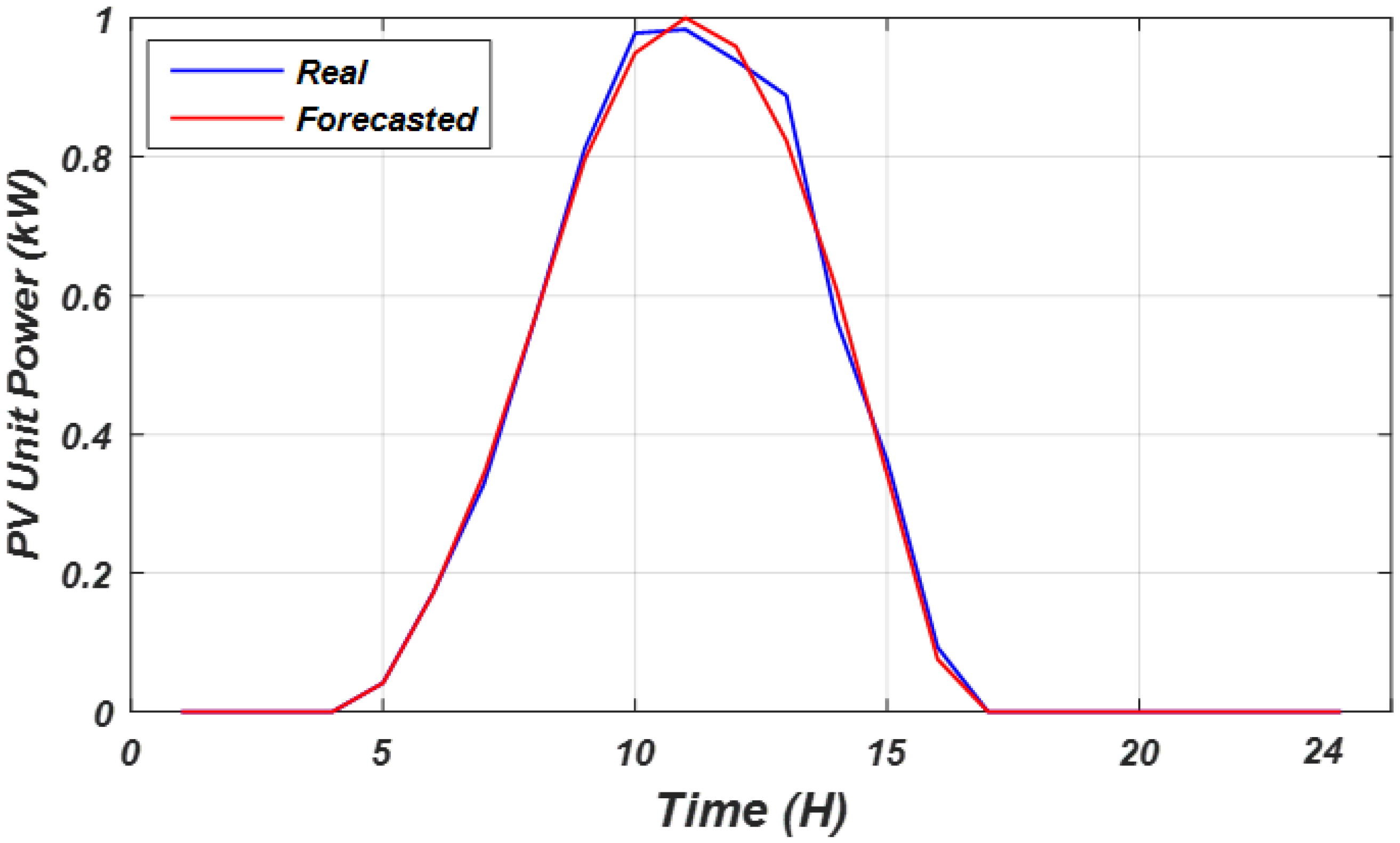
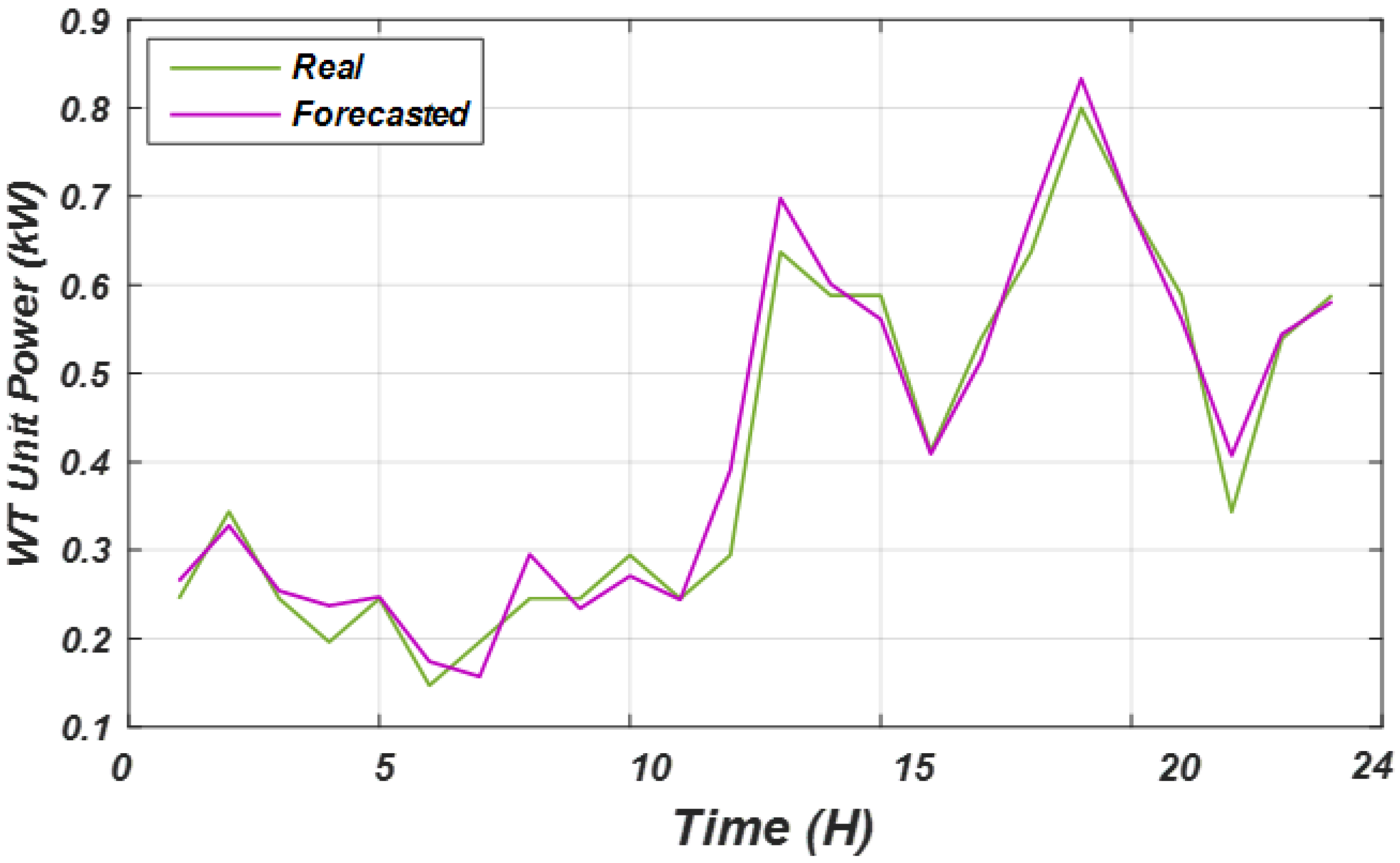
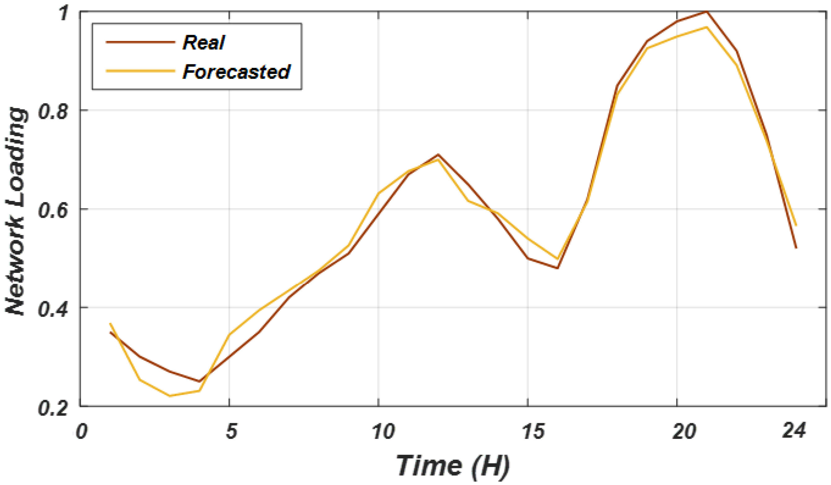
As shown, the ESCHO-ANN accurately forecasts PV and WT unit power and network loading. The ESCHO-ANN was trained on real data from solar and wind sites in the Dammam area of Saudi Arabia (26°26′3.9″ N, 50°6′11.74″ E) [36]. These data provide the meteorological parameters needed to train the model for forecasting variables used in distribution-network optimization, such as renewable unit power and network loading. Forecasts produced by ESCHO-ANN are compared with observations and are presented in Figure 2, Figure 3 and Figure 4, respectively.

Figure 2. The normalized PV unit power during a day.

Figure 3. The normalized WT unit power during a day.

Figure 4. The normalized distribution network loading during a day.

2.5. Proposed Stochastic Approach

The Unscented Transformation (UT) [37] method selects 2n + 1 sigma points to approximate the input distribution and compute the output mean and covariance. Although the method is more computationally efficient than Monte Carlo simulation, in high-dimensional problems, the number of sigma points grows linearly with dimension, and the computational cost can become excessive. As an alternative to this, the Cubature Quadrature Rule (CQR) [38] is introduced. The strength of CQR lies in calculating the required multidimensional integrals for statistical moments not through large random sampling but by using a small number of cubature points, placed centrally around the distribution mean. To achieve this, UT-CQR combines the simplicity of UT and the efficiency of CQR and achieves high accuracy with fewer points. The reason for using the UT-CQR framework is the reduced efficiency of the conventional UT when applied to high-dimensional stochastic systems.

Although UT is an efficient substitute for Monte Carlo sampling using a deterministic collection of sigma points, its computational complexity scales with system dimension (2n + 1 points). CQR addresses this issue by replacing sigma points with symmetrically ordered cubature points, requiring 2n evaluations without loss of accuracy. With balanced and symmetric integration, CQR improves covariance and mean estimation, numerical stability, and preservation of higher-order moment information. With these improvements, the use of CQR with UT not only alleviates the computational burden but also significantly improves computational efficiency and accuracy in uncertainty transfer, and hence is of particular interest for the analysis of large-scale nonlinear distribution systems. Let the input random vector be $x\in {\mathbb{R}}^n$ with mean ${\mu }_x$ and covariance σx. The objective is to estimate the transformed mean and covariance of the nonlinear mapping $y=f\left(x\right)$.

• Cubature point selection

A symmetric collection of 2n cubature points around the mean is created as follows:

$$X_i={\mu }_x+\sqrt{n}\cdot e_i,\hspace{1em}i=1,\dots ,n$$

(27)

$$X_{i+n}={\mu }_x-\sqrt{n}\cdot e_i,\hspace{1em}i=1,\dots ,n$$

(28)

where e_i is the ith unit basis vector in Rⁿ. This construction ensures third-order exact integration of polynomials.

• Propagation through the nonlinear function

Every cubature point is mapped by the nonlinear function as follows:

$$Y_i=f\left(X_i\right),\hspace{1em}i=1,\dots ,2n$$

(29)

• Mean estimation

The mean of the transformed distribution is obtained as follows:

$${\mu }_y={\displaystyle \frac{1}{2n}}\sum _{i=1}^{2n}{Y}_i$$

(30)

• Covariance estimation

The covariance of the transformed distribution is as follows:

$${\sigma }_y={\displaystyle \frac{1}{2n}}\sum _{i=1}^{2n}(Y_i-{\mu }_y)(Y_i-{\mu }_y{)}^T$$

(31)

Pseudocode of the UT-CQR approach is given in Algorithm 1.

Algorithm 1. Pseudocode of the UT-CQR approach

Input:     Mean of input state: μ_x     Covariance of input state: σ_x     Dimension of state: n     Nonlinear function: f(·) Step 1: Generate Cubature Points     For i = 1 to n:         X_i      = μ_x + sqrt(n) * e_i         X_(i+n) = μ_x − sqrt(n) * e_i     End     Total cubature points = 2n Step 2: Propagation Through Nonlinear Function     For each point X_i:         Y_i = f(X_i)     End Step 3: Compute Mean of Output     μ_y = (1/(2n)) * Σ (Y_i), i = 1 to 2n Step 4: Compute Covariance of Output     σ_y = (1/(2n)) * Σ ((Y_i − μ_y)(Y_i − μ_y)^T), i = 1 to 2n Output:     Estimated mean μ_y     Estimated covariance σ_y

3. Numerical Results and Discussion

3.1. System Data and Simulation Cases

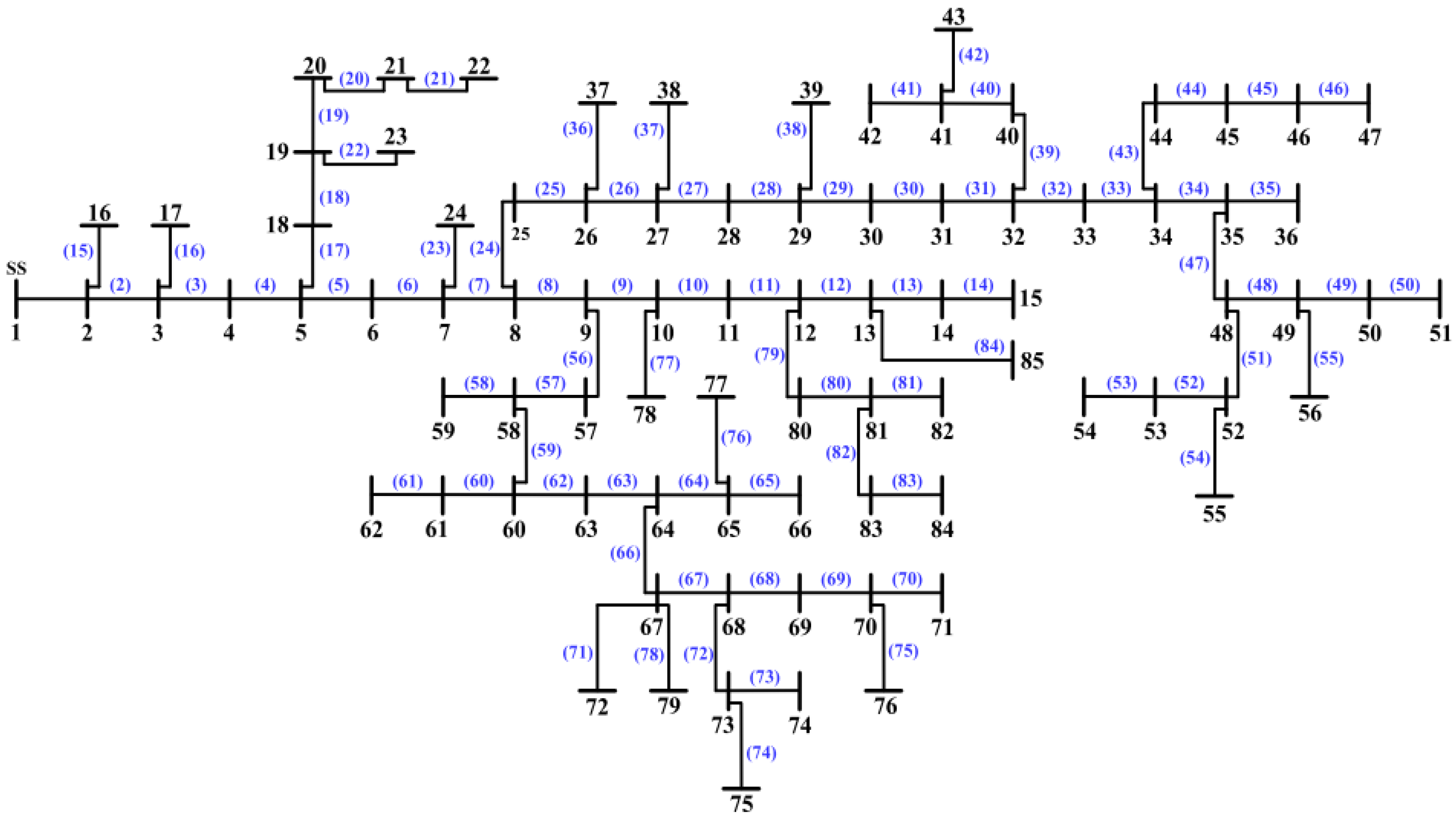
In the present study, results of emission- and reliability-aware stochastic optimization of EBPLs and WT–PV are presented for a radial 85-bus distribution system (Figure 5) using a fuzzy decision-making multi-objective approach based on real and forecasted data and uncertainty handled by MO-ESCHO. The 85-bus distribution system has loads of 2570.28 kW and 2622.08 kVAr with 84 lines at a nominal voltage of 11 kV, with bus and line data adopted from [39]. The energy-loss cost and grid cost in this work are assumed to be 0.06 USD/kWh and 0.096 USD/kW, respectively [40]. Maximum capacity for WT and PV is considered to be 2 MW, and the EBPL capacity is 3.5 MWh, respectively. The PV arrays are assumed to be fixed-tilt systems at the optimum tilt angle corresponding to the site latitude and facing south for maximum annual energy production. All PV arrays in the plant (maximum capacity of 2 MW) operate under standard test conditions (STC) with an inverter efficiency of 96% and are connected to the distribution feeder through a three-phase inverter interface. Also, the ENS penalty cost is taken as 0.5 USD/kWh. For calculation of reliability, the failure rate of each line is taken as 0.02 failures/year, and the repair time is 8 h [41]. Cost values for unit power of WT, PV, and EBPL purchased by the distribution network are shown in Table 3. The proposed MO-ESCHO is compared with MO-SCHO, MO-PSO, and MO-SCA algorithms. The population size, iterations, and independent runs of each algorithm are set to 50, 200, and 20, respectively. Algorithm control parameters are shown in Table 4 [42,43]. The implemented methodology is coded in MATLAB 2015b and executed on a desktop computer with an Intel Core i7-4510U processor [Intel, Beijing, China] (up to 3.1 GHz), 1 TB HDD, and a 64-bit Windows 8 operating system.

Figure 5. Single diagram of 85-bus distribution network (blue numbers refer to the network lines number).

Table 3. The cost details of PV, WT, and EBPL unit capacity [40,41].

Device	Value
PV unit power cost (USD/kW)	0.045
WT unit power cost (USD/kW)	0.070
EBPL unit energy cost (USD/kWh)	0.055

Table 4. Control parameters of each algorithm.

Algorithm	Parameter	Value
SCHO [33]	Sensitive variable, u Constant parameter, m Coefficient, n	0.388 0.45 0.5
PSO [42]	Inertia weight Cognitive and social factors	Linear decrease from 0.9 to 0.1 2, 2
SCA [43]	r1	Decreases linearly from 2 to 0

The test cases of the proposed methodology are as follows:

Case I: RES without EBPL + real data: The distribution network operates solely on RES (PV and wind) without EBPL. Actual historical data are used to evaluate performance. This serves as a benchmark for assessing the impact of EBPL and other measures.

Case II: RES with EBPL + real data: EBPL is incorporated alongside RES, again using real data. This case quantifies EBPL effects on operating cost, energy losses, and reliability, and is compared with Case I to measure the benefits of EBPL integration.

Case III: RES with EBPL + real data + DR: In addition to RES and EBPL, a demand-response (DR) strategy using realistic data is applied. DR enables load shifting based on network conditions to improve efficiency, reduce operating costs, and further enhance reliability. This case evaluates the joint impact of EBPL and DR.

Case IV: RES with EBPL + forecasted data + DR: RES, EBPL, and DR are considered with forecasted PV, wind, and load data. This case analyzes predictive-mode performance and the effect of forecast accuracy on optimization outcomes, energy losses, operating cost, and reliability.

Case V: RES with EBPL + forecasted data + DR + stochastic modeling: This case extends Case IV with stochastic modeling to capture uncertainty in PV and wind generation and in network load. It evaluates the robustness of the optimization framework and its ability to deliver reliable, emission-aware solutions under real-world uncertainty. Considered uncertainties include PV fluctuations driven by seasonal solar-irradiance variability, wind-power variability due to changing wind speeds, and customer-demand variations affecting network load.

3.2. Results of Case I, RES Without EBPL with Real Data

For this case, the system is optimized with RES, i.e., solar and wind, using actual data, but without EBPL. The primary objective is to minimize operating cost, emission cost, and ENS while keeping the network reliable. For this case, the Pareto-front solution is presented, showing the trade-off among operating cost, emission cost, and ENS for the optimization without EBPL. The Pareto front in Figure 6 presents various combinations of the objectives, delineating the relationship between operating cost, emission cost, and reliability based on ENS. As shown, emission cost increases nearly linearly with operating cost, while ENS remains relatively flat across the solution set. This analysis outlines how different RES (PV and WT) configurations affect the objectives and provides a baseline for comparison when EBPLs and DR are incorporated.

Figure 6. Pareto front solution set for case I (blue circles refer to the Pareto solution set).

A comparison of optimization results for Case I using the algorithms MO-ESCHO, MO-SCHO, MO-PSO, and MO-SCA is presented in Table 5. The comparison covers key parameters, including PV and WT size, operating cost, emission cost, ENS, and energy-loss cost. MO-ESCHO achieves the lowest emission cost of USD 360,474,505.31, a 56.2% reduction relative to the Base Network (USD 822,276,015.03). It also yields the lowest operating cost of USD 1,237,651.10, slightly lower than MO-SCHO at USD 1,241,651.10. Considering energy-loss costs, MO-ESCHO performs better with USD 56,768.30, a 41.3% reduction from the Base Network (USD 96,732.12). For ENS, MO-ESCHO delivers 39.63 MWh, with MO-SCHO second at 39.93 MWh, matching the Base Network’s value of 39.63 MWh. These results show that MO-ESCHO greatly reduces emission and energy-loss costs while improving network reliability. The results also confirm that integrating RES into the distribution network is more energy-efficient and cost-effective than the Base Network.

Table 5. Optimization results for case I.

Item/Value	Base Network	MO-ESCHO	MO-SCHO	MO-PSO	MO-SCA
PV Size (kW)/@PV Site (Bus)	--	2000/@4	2000/@4	2000/@57	2000/@57
WT Size (kW)/@WT Site (Bus)	--	1596.07/@20	1612.65/@46	1600.36/@8	1585.65/@25
Operating Cost (USD)	--	1,237,651.10	1,241,651.10	1,239,515.50	1,240,592.67
Emission Cost (USD)	822,276,015.03	360,474,505.31	371,739,026.25	368,863,911.58	372,502,114.25
Energy Not Supplied (MWh)	58.74	39.63	39.93	39.72	39.90
Energy Loss Cost (USD)	96,732.12	56,768.30	57,214.35	57,125.14	57,266.17
PV Cost (USD)	--	219,150.00	219,150.00	219,150.00	219,150.00
WT Cost (USD)	--	755,072.30	761,375.16	756,240.36	751,083.44
Hypervolume	--	0.8627	0.8453	0.8571	0.8460
Spacing	--	0.2356	0.2459	0.2411	0.2438

In Figure 7, the power injected into the distribution system by PV, WT, and the grid for a 24 h period is shown. The PV power peaks around noon at approximately 2000 kW and then declines as the sun sets. WT power fluctuates with wind conditions, is somewhat irregular, and generally remains below PV output, peaking slightly above 1500 kW. The third plot shows grid power consumed to meet residual demand when renewable generation is insufficient. Thus, the grid provides additional power when renewable generation is inadequate, and the system relies on the grid at night or during low renewable output. This reflects the effectiveness of integrating RES into the system. The grid supply bridges the gap, while the PV and WT systems reduce grid dependency, particularly during peak renewable output periods. Through optimal utilization of RES, the system can significantly reduce its dependency on the grid, as reflected in the power balance.

Figure 7. Power injected to distribution network by the PV (red), WT (green), and grid (blue) for Case I.

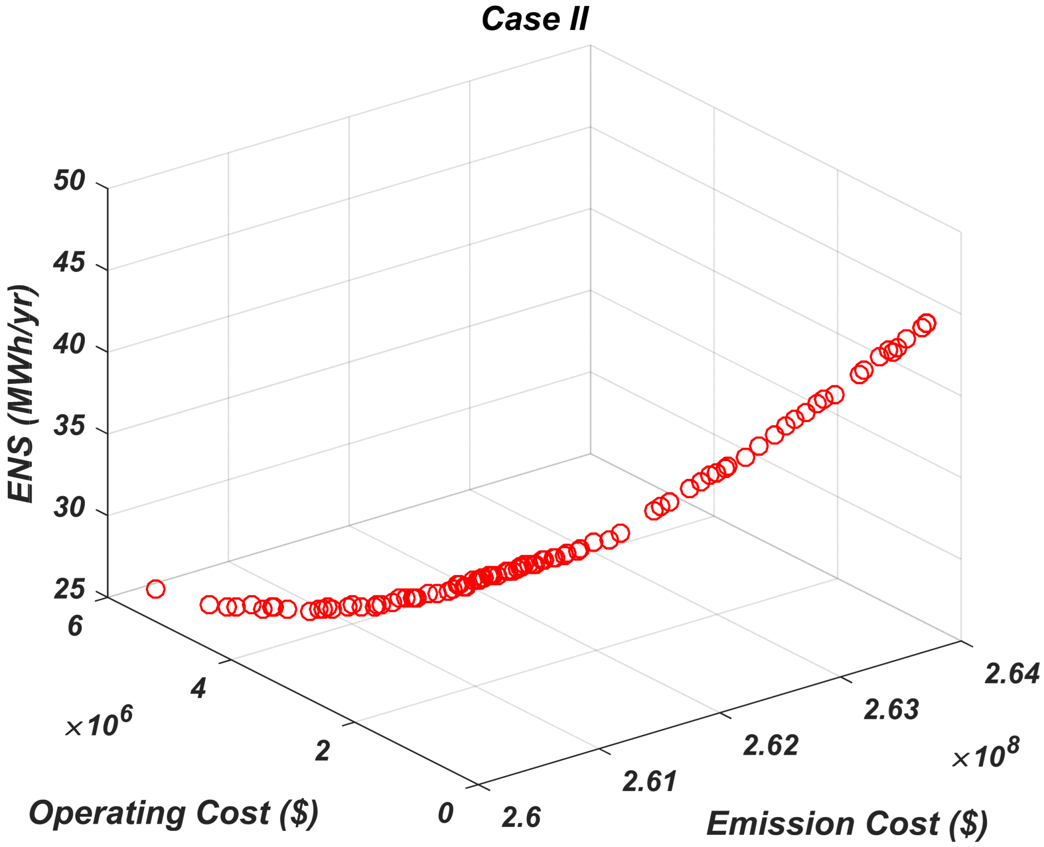
For Case II, the optimization considers integrating EBPL with RES (WT and PV) using real data.

The goal is to quantify how EBPL contributes to reducing operating costs, emission costs, energy losses, and ENS while maintaining reliability. The Pareto front in Figure 8 shows the trade-offs: higher operating costs correspond to higher emission costs, whereas ENS remains relatively constant. EBPL integration enhances energy storage and dispatch flexibility, reducing costs and emissions. Overall, EBPL integration leads to a more balanced and efficient system operation.

Figure 8. Pareto front solution set for case II (red circles refer to the Pareto solution set).

Table 6 presents a comparison of optimization results for Case II using the algorithms MO-ESCHO, MO-SCHO, MO-PSO, and MO-SCA. The table reports PV and WT capacities, EBPL capacity, operating cost, emission cost, ENS, energy-loss cost, and other parameters for all algorithms. MO-ESCHO yields the lowest emission cost of USD 261,716,433.24, a 68.2% reduction relative to the Base Network (USD 822,276,015.03). This substantial reduction indicates the effectiveness of MO-ESCHO in minimizing emissions with RES and EBPL integration. In addition, MO-ESCHO achieves the lowest operating cost of USD 1,172,889.61, marginally better than MO-SCHO’s USD 1,181,573.58.

Table 6. Optimization results for case II.

Item/Value	Base Network	MO-ESCHO	MO-SCHO	MO-PSO	MO-SCA
PV Size (kW)/@Site (Bus)	--	2000/@5	2000/@21	1992/@32	1886/@60
WT Size (kW)/@Site (Bus)	--	1605.12/@28	1611.58/@27	1637.36/@61	1792.15/@34
EBPL Size (kW)/@Site (Bus)	--	3115/@32	3133/@60	3104/@12	3162/@51
Operating Cost (USD)	--	1,172,889.61	1,181,573.58	1,177,246.01	1,179,536.40
Emission Cost (USD)	822,276,015.03	261,716,433.24	265,735,803.72	262,762,118.25	264,342,500.66
Energy Not Supplied (MWh)	58.74	35.08	35.73	35.46	35.59
Energy Loss Cost (USD)	96,732.12	37,683.897	37,924.76	37,794.18	37,764.36
PV Cost (USD)	--	219,150.00	219,150.00	217,820.73	201,905.96
WT Cost (USD)	--	716,686.22	718,527.35	726,922.86	788,482.85
EBPL Charge Cost (USD)	--	46,619.27	62,897.61	622,904.20	64,157.08
EBPL Discharge Cost (USD)	--	33,927.40	34,520.08	44,327.91	31,512.37
Hypervolume	--	0.8741	0.8639	0.8652	0.8663
Spacing	--	0.2157	0.2293	0.2285	0.2276

Compared to the Base Network, the reduction in operating cost is also evident, further supporting the value of EBPL integration. MO-ESCHO also achieves the lowest energy-loss cost of USD 37,683.897, which is 61.1% lower than the Base Network’s USD 96,732.12. This indicates that the incorporation of EBPL and RES significantly reduces energy losses and improves overall network efficiency. For ENS, the best performer is MO-ESCHO at 35.08 MWh, slightly improving on MO-SCHO at 35.73 MWh. Both algorithms outperform the Base Network, demonstrating that EBPL and RES reduce ENS. The reduction in ENS highlights the role of energy storage (via EBPL) in reinforcing network reliability and reducing the likelihood of power shortages. The EBPL charging and discharging costs are also reported. MO-ESCHO yields a charging cost of USD 46,619.27 and a discharging cost of USD 33,927.40. These reflect EBPL’s contribution to the overall process of power distribution and storage, maximizing benefits while minimizing losses and costs.

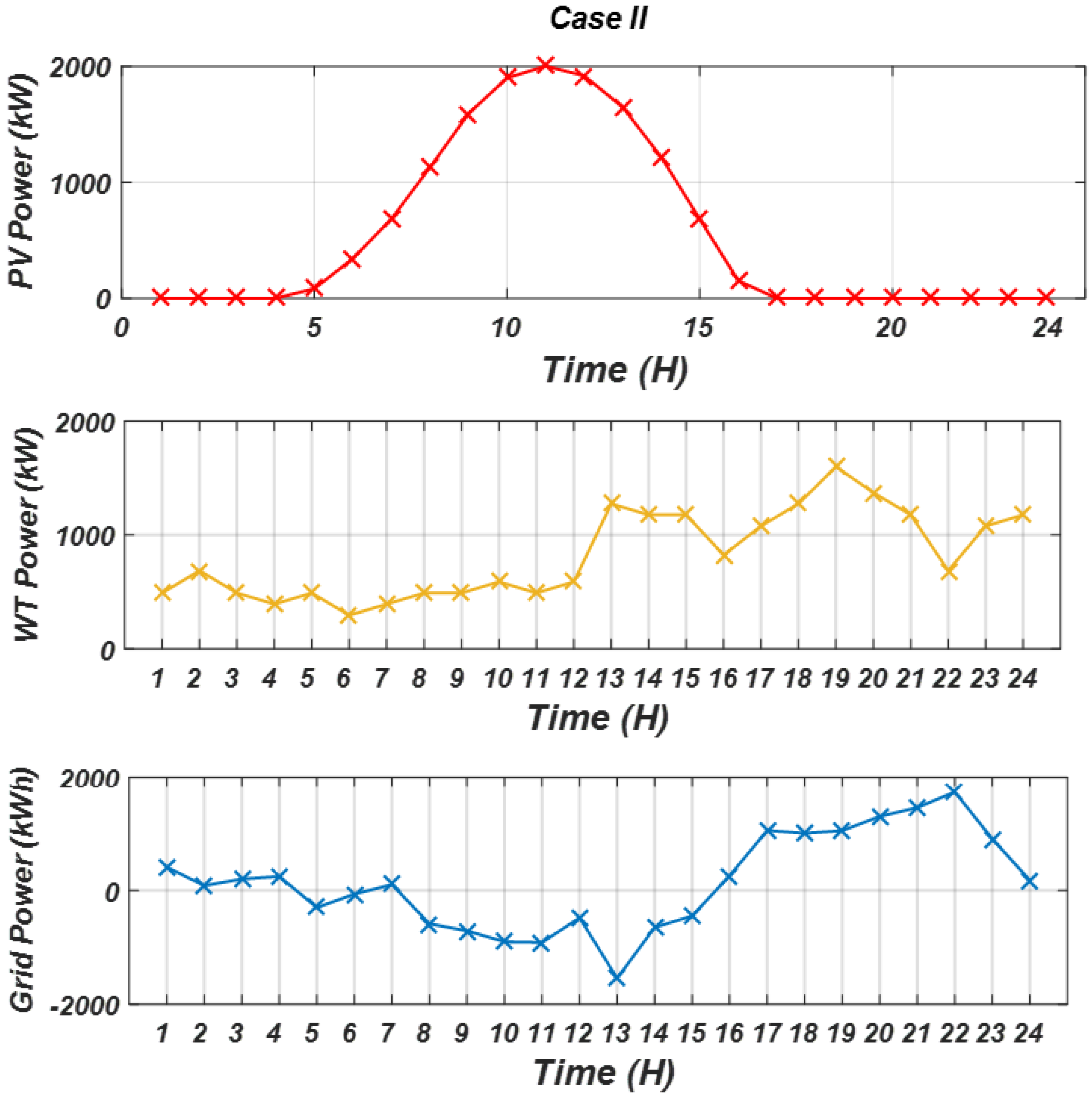
Figure 9 shows the power contributions from PV, WT, and the grid during a 24 h period. The top panel shows PV generation, which peaks in the middle of the day with maximum power around 12:00. The second panel represents WT output, which varies day to day with changing wind conditions. The third panel shows grid power, the supply required when RES generation is insufficient to cover demand. Overall, the combination of PV and WT substantially reduces grid dependency, particularly during peak PV hours. This confirms the effectiveness of RES with EBPL in reducing grid dependency.

Figure 9. Power injected to distribution network by the PV (red), WT (orange), and grid (blue) for Case II.

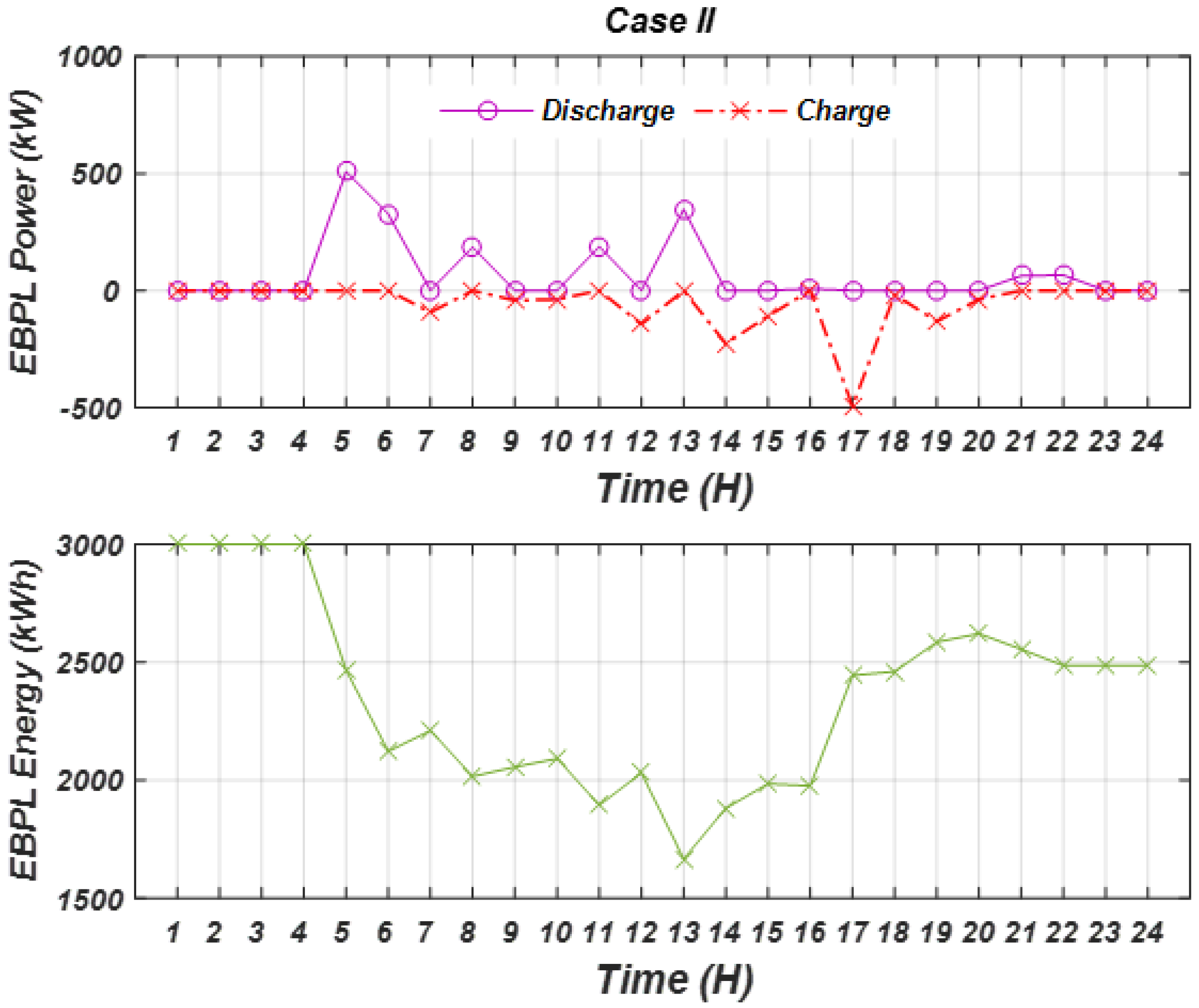
EBPL charging and discharging patterns and the stored-energy profile over a 24 h horizon are shown in Figure 10. The top curve shows charging and discharging power, peaking when energy is delivered to or drawn from the EBPL. The bottom curve shows the stored energy, which accumulates during periods of high PV or WT output and decreases when energy is supplied to the grid. The inclusion of an EBPL improves supply–demand matching and helps ensure energy availability during periods of lower RES output.

Figure 10. EBPL charge and discharge power as well as its energy changes (green) during a day for Case II.

3.3. Results of Case III, RES with EBPL and DR

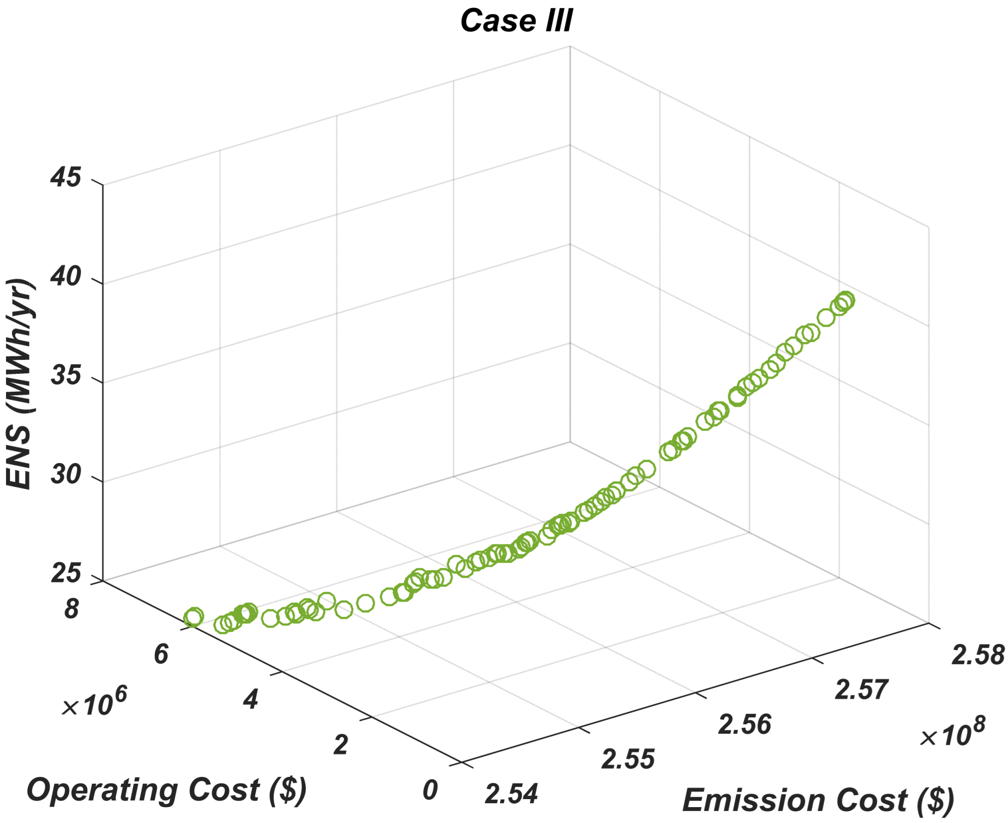
For Case III, the optimization includes EBPL, RES (WT and PV), and DR with actual data. The aim is to study their combined impact on operating cost, emission cost, energy loss, and ENS, while maintaining reliability. Figure 11 shows the Pareto front, which illustrates the trade-offs among these objectives. As in earlier examples, operating and emission costs increase simultaneously, whereas the inclusion of EBPL and DR reduces ENS and improves overall performance. Overall, the results show that integrating EBPL and DR enhances system efficiency and sustainability through a more efficient energy-distribution plan.

Figure 11. Pareto front solution set for case III (green circles refer to the Pareto solution set).

Table 7 presents the optimization results for Case III using four algorithms as follows: MO-ESCHO, MO-SCHO, MO-PSO, and MO-SCA. The comparison includes key parameters such as PV and WT unit sizes, EBPL capacity, operating cost, emission cost, ENS, and energy-loss cost. MO-ESCHO shows the best performance, achieving a minimum emission cost of USD 255,709,362.56, which represents a 31.5% decrease from the Base Network value of USD 37,440,173.00. This reflects the algorithm’s capability to significantly decrease emissions with optimized operating costs. In addition, MO-ESCHO yields the lowest operating cost of USD 1,128,894.06, slightly lower than MO-SCHO’s USD 1,131,573.58, representing a 3.4% reduction from the base case.

Table 7. Optimization results for case III.

Item/Value	Base Network	MO-ESCHO	MO-SCHO	MO-PSO	MO-SCA
PV Size (kW)/@Site (Bus)	--	2000/@5	1980.78/@41	1957/@21	1971/@21
WT Size (kW)/@Site (Bus)	--	1600.04/@28	1589.14/@20	1631.04/@47	1689.04/@27
EBPL Size (kW)/@Site (Bus)	--	3148/@29	3082/@69	3156/@43	3101/@43
Operating Cost (USD)	--	1,128,894.06	1,142,975.44	1,130,705.21	1,140,575.49
Emission Cost (USD)	822,276,015.03	255,709,362.56	257,200,346.08	257,110,226.32	257,184,223.37
Energy Not Supplied (MWh)	58.74	34.11	34.35	34.26	34.31
Energy Loss Cost (USD)	96,732.12	36,597.84	37,088.53	36,754.68	36,915.34
PV Cost (USD)	--	219,150.00	216,715.27	214,281.33	211,428.40
WT Cost (USD)	--	687,793.15	681,014.93	674,104.02	690,371.87
DR Cost (USD)	--	31,107	33,536	31,560.75	31,744.06
EBPL Charge Cost (USD)	--	39,081.58	41,915.22	42,536.41	41,885.24
EBPL Discharge Cost (USD)	--	30,175.90	37,631.84	30,175.90	30,128.01
Hypervolume	--	0.8976	0.8473	0.8420	0.8478
Spacing	--	0.1932	0.1975	0.1964	0.1979

In terms of energy-loss cost, MO-ESCHO achieves the lowest value of USD 36,597.84, a reduction of 62.2% from the Base Network’s USD 96,732.12, indicating higher system efficiency when EBPL and RES are used together.

For ENS, the best result is achieved by MO-ESCHO at 34.11 MWh, closely followed by MO-SCHO at 34.35 MWh, with both algorithms showing substantial improvements over the baseline network and, thus, improving reliability.

EBPL charging and discharging costs are also reported: MO-ESCHO yields a charging cost of USD 39,851.58 and a discharging cost of USD 30,775.90, reflecting EBPL operating costs and the energy balancing it provides.

Regarding performance indicators, Hypervolume and Spacing are used to measure optimization quality. MO-ESCHO has the highest Hypervolume at 0.8976, followed by MO-PSO at 0.8652, indicating a more Pareto-optimal and diverse set of solutions. The Spacing index, which measures solution uniformity, is lowest for MO-ESCHO at 0.1932, meaning its Pareto-front distribution is more uniformly spaced compared to other algorithms. In general, these findings further confirm MO-ESCHO’s dominance in producing well-distributed, diverse, and effective optimization outcomes across all objectives.

Figure 12 for Case III shows the 24 h power contributions from PV, WT, and the grid. PV power follows a typical daily cycle, peaking at approximately 2000 kW around midday, while WT power varies with wind conditions, peaking around 1000 kW. The grid supplies power mostly at night and during periods of low renewable output. The integration of PV, WT, and grid power, supported by EBPL and DR, improves energy management by reducing grid dependence during peak renewable availability and increasing overall system efficiency.

Figure 12. Power injected to distribution network by the PV (orange), WT (red), and grid (green) for Case III.

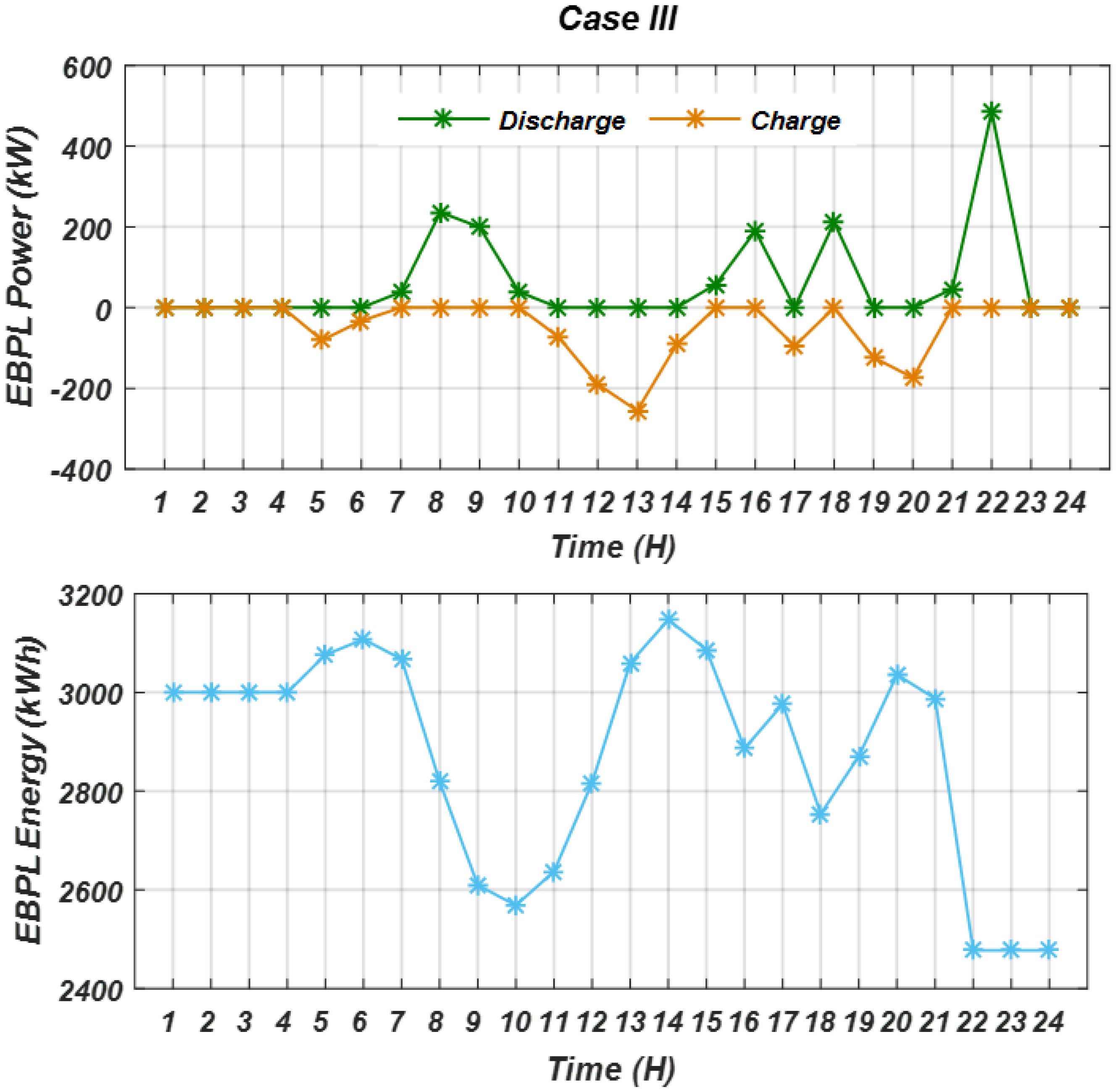
The EBPL charging and discharging power with its stored energy over a 24 h period are shown in Figure 13. The upper panel illustrates the charging process when there is abundant RES output and the discharging process during peak-demand hours. The lower panel indicates the fluctuation of stored energy in the EBPL, which increases during periods of abundant renewable generation and decreases when energy is fed to the grid to compensate for lower RES production.

Figure 13. The EBPL charge and discharge power as well as its energy changes (blue) during a day for Case III.

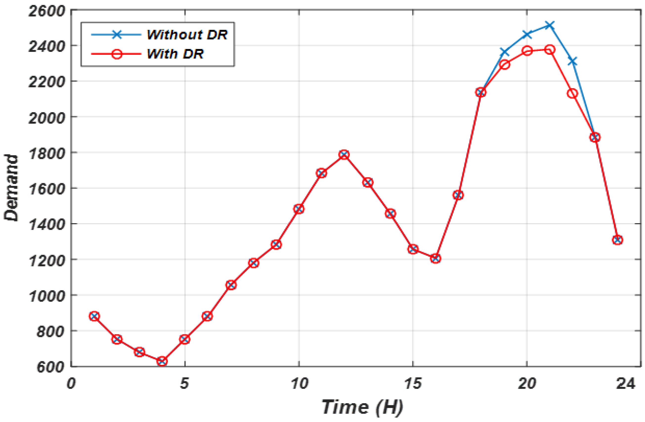
Figure 14 shows a load-demand profile for Case III with and without demand response (DR). The use of DR successfully redistributes demand, lowering peak loads and smoothing the profile. This is evident from the deviation between the “without DR” (blue) and “with DR” (red) curves. By smoothing demand during peak hours, DR reduces grid stress, enhances system reliability, and decreases the need for backup grid power.

Figure 14. The load demand without and with DR for Case III.

3.4. Results of Case IV, RES with EBPL Under Forecasted Data

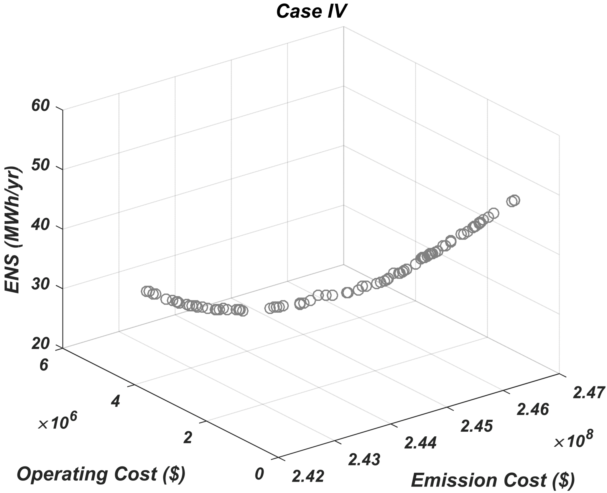
In Case IV, the integration of EBPL with forecasted renewable generation and load data enables more effective system optimization. The Pareto front (Figure 15) results have improved trade-offs, with operational cost held steady while emission cost and ENS are reduced. This demonstrates the benefit of accurate forecasting combined with EBPL to provide balanced, reliable, and sustainable energy management.

Figure 15. Pareto front solution set for case IV (grey circles refer to the Pareto solution set).

Case IV includes the integration of EBPL, RES, and forecasted data for optimization. The comparison of optimization results for MO-ESCHO, MO-SCHO, MO-PSO, MO-SCA, NSGA-II, and the Base Network in Table 8 provides system-performance details for important parameters such as operating cost, emission cost, energy-loss cost, ENS, and the costs of PV, WT, and EBPL. The MO-ESCHO algorithm achieves the lowest operating cost of USD 1,080,464.50, significantly lower than the Base Network at USD 1,172,889.61. This represents a 7.9% reduction in operating cost. MO-ESCHO performs best at minimizing operating cost compared with the other algorithms: MO-SCHO at USD 1,135,574.21, MO-PSO at USD 1,110,937.53, and MO-SCA at USD 1,112,283.27.

Table 8. Optimization results for case IV.

Item/Value	Base Network	MO-ESCHO	MO-SCHO	MO-PSO	NSGA-II	MO-SCA
PV Size (kW)/@Site (Bus)	--	1966.49/@5	1874.73/@5	2000/@61	2000/@61	2000/@61
WT Size (kW)/@Site (Bus)	--	1668.53/@9	1776.94/@29	1689.11/@29	1692.53/@29	1794.65/@26
EBPL Size (kW)/@Site (Bus)	--	3235.23/@16	3495.38/@46	3105.35/@24	3117.31/@46	2850.71/@44
Operating Cost (USD)	--	1,080,464.50	1,135,574.21	1,110,937.53	1,118,732.38	1,112,283.27
Emission Cost (USD)	822,276,015.03	244,394,019.89	246,175,914.50	244,734,118.06	244,966,504.14	244,966,720.48
Energy Not Supplied (MWh)	58.74	32.36	33.15	32.57	32.64	32.83
Energy Loss Cost (USD)	96,732.12	37,231.87	39,463.82	37,472.28	37,506.95	37,885.61
PV Cost (USD)	--	213,150.00	205,339.20	219,150.00	219,150.00	219,150.00
WT Cost (USD)	--	656,686.10	685,178.18	661,186.65	661,288.91	692,186.65
EBPL Charge Cost (USD)	--	62,007.44	60,400.06	61,929.80	61,947.33	56,122.07
EBPL Discharge Cost (USD)	--	41,698.82	38,248.03	40,056.71	40,107.56	37,883.61
Hypervolume	--	0.8930	0.8829	0.8875	0.8859	0.8842
Spacing	--	0.1945	0.1988	0.1976	0.1980	0.1982

The emission cost for MO-ESCHO is USD 244,394,019.89, a 70.3% reduction from the Base Network’s USD 822,276,015.03. This indicates strong emission-reduction performance, consistent with comparisons to the other algorithms. MO-SCHO and MO-PSO also achieve large reductions, with costs of USD 246,175,914.50 and USD 244,734,118.06, respectively. These reductions indicate the positive impact of integrating RES and EBPL. MO-ESCHO’s ENS is 32.36 MWh, much lower than the Base Network at 58.74 MWh, a reduction of 44.9%. MO-SCHO follows with 33.15 MWh and MO-PSO with 32.57 MWh, both improving on the Base Network. Energy-loss cost is lowest for MO-ESCHO at USD 37,231.87, a 61.5% reduction from the Base Network at USD 96,732.12. This reduction underscores the efficacy of MO-ESCHO in reducing system losses. The remaining algorithms have higher energy-loss costs: MO-SCHO at USD 39,463.82, MO-PSO at USD 38,248.03, MO-SCA at USD 37,885.61, and NSGA-II at USD 37,506.95.

MO-ESCHO has a PV cost of USD 213,150.00, which is higher than the Base Network (no PV). The remaining algorithms report comparable PV costs, with MO-SCHO at USD 205,339.20 and MO-PSO at USD 219,150.00. WT cost: MO-PSO provides the highest WT cost of USD 718,527.35, followed by MO-ESCHO with USD 656,686.10 and MO-SCHO with USD 685,178.18. EBPL charge and discharge costs: MO-ESCHO reports a charging cost of USD 62,007.44 and a discharging cost of USD 41,698.82, representing the cost of charging and discharging energy in the EBPL system.

In optimization metrics, MO-ESCHO outperforms the other algorithms in both Hypervolume and Spacing. MO-ESCHO has a Hypervolume of 0.8930, exceeding MO-SCHO at 0.8829 and MO-PSO at 0.8857. This indicates that MO-ESCHO provides a broader range of Pareto-optimal solutions, enhancing solution diversity. The Spacing index of MO-ESCHO is also the lowest at 0.1945, meaning its solutions are more evenly distributed along the Pareto front, compared to MO-SCHO at 0.1988, MO-PSO at 0.1964, and MO-SCA at 0.1979. The lower Spacing value indicates that MO-ESCHO has a more uniform distribution of solutions, and therefore is preferable for obtaining a well-distributed trade-off between objectives.

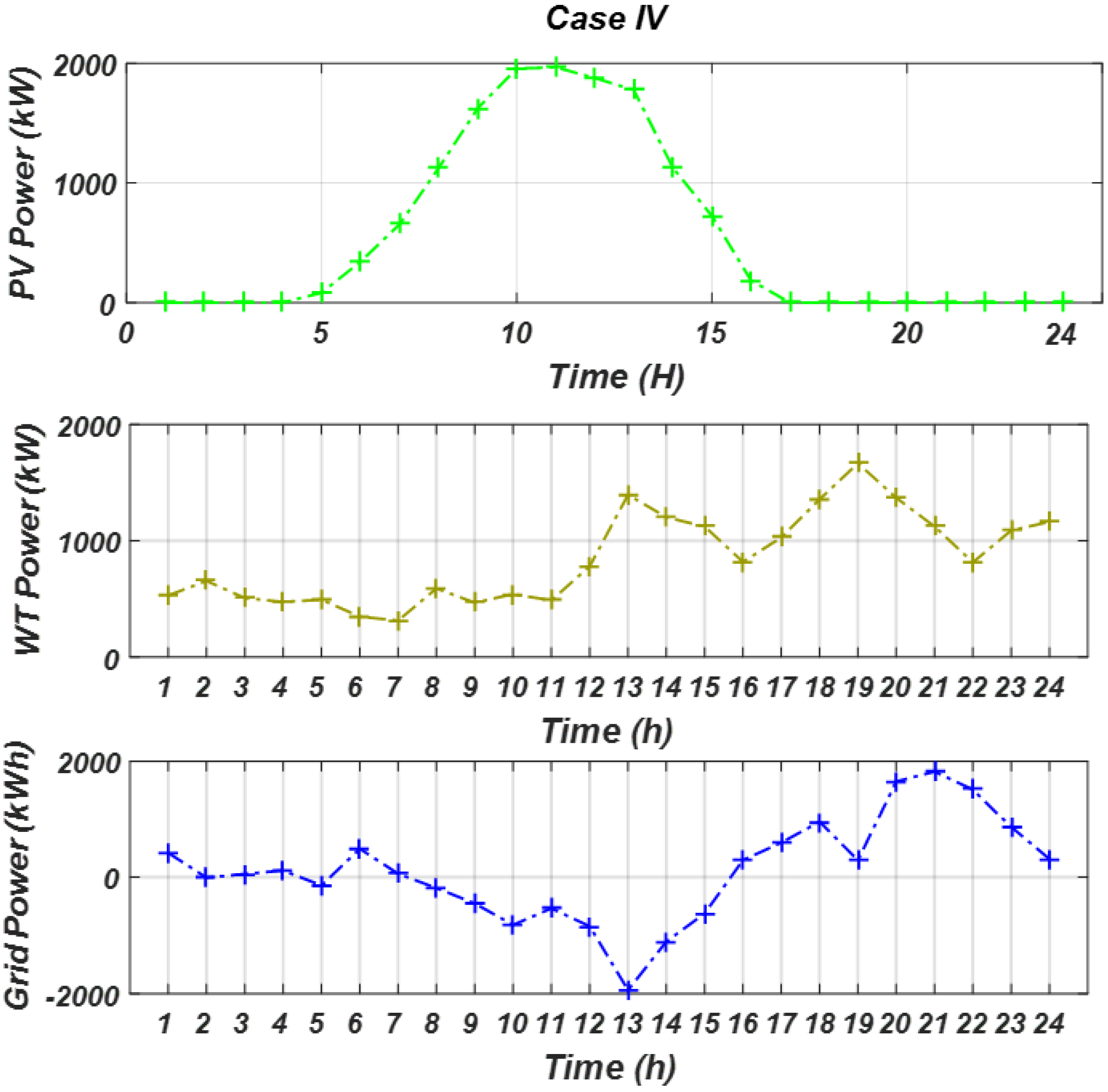
Figure 16 illustrates the 24 h power output of PV, WT, and the grid in Case IV. PV output follows a standard solar curve, peaking at noon and declining in the evening. WT power varies throughout the day, with peaks at different times depending on wind availability. The grid supplies additional power mainly at night when solar output decreases. This indicates how EBPL, along with RES, reduces dependence on the grid by storing excess energy during periods of high renewable generation and discharging it when demand exceeds generation.

Figure 16. Power injected to distribution network by the PV (green), WT (brown), and grid (blue) for Case IV.

Figure 17 shows the EBPL charge/discharge power and stored energy over a 24 h period. The upper panel shows charging during high PV and WT generation and discharging as demand rises or renewable generation falls. The lower panel shows stored energy, which accumulates during high renewable output and draws down as it feeds energy back into the system. This demonstrates EBPL’s role in optimizing energy management by stabilizing fluctuations in renewable availability and contributing to a smoother supply–demand equilibrium.

Figure 17. The EBPL charge and discharge power as well as its energy changes (green) during a day for Case IV.

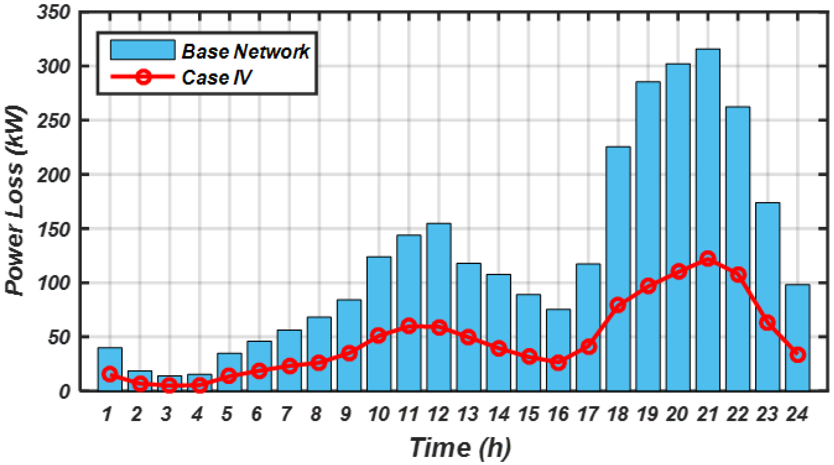
Figure 18 compares the power loss in the distribution network before and after improvement for Case IV. Blue bars represent the Base Network, which experiences higher power loss, especially during peak demand hours. The red line represents Case IV, showing a significant reduction in power loss due to the integration of RES and EBPL. The optimization has managed to minimize the energy loss, depicting the benefits of the utilization of RES and EBPL in improving system efficiency and reducing energy loss.

Figure 18. The power loss of distribution network before (Base Network) and after optimization for Case IV.

The quantitative results given in Table 9 strongly confirm the improved operational and environmental performance of RES with EBPL (Case IV) configuration compared to the RES-with-EVPL system. In terms of operating cost, the EBPL-based case records an operating cost of USD 1,080,464.50, approximately 2.5% lower than that of the EVPL-based setup (USD 1,107,520.13) due to more coordinated and predictable charging–discharging patterns of EBs that allow efficient utilization of renewable energy and reduced reliance on grid purchases. The emission cost also decreases considerably, falling to USD 244.39 million from USD 244.57 million for EVPL, in response to increased renewable energy integration and smoother load management, reducing fossil-based generation. Moreover, the energy not supplied (ENS) falls from 33.19 MWh for EVPL to 32.36 MWh for EBPL integration, which indicates higher system reliability and improved supply adequacy. Also, the energy-loss cost decreases from USD 37,455.82 to USD 37,231.87, reflecting the ability of the EBPL model to reduce distribution losses by localizing renewable generation and optimizing load flow. Taken together, these enhancements highlight that the RES with EBPL (Case IV) arrangement provides a lower-cost, more reliable, and greener operating performance than the EVPL-based system, confirming the technical and economic advantages of adopting EBPLs as flexible, centrally controlled energy sources in smart distribution networks.

Table 9. Comparison of EBPL and EVPL applications with the RES.

Item/Value	Base Network	RES with EBPL (Case IV)	RES with EVPL
PV Size (kW)/@Site (Bus)	--	1966.49/@5	2000/@61
WT Size (kW)/@Site (Bus)	--	1668.53/@9	1695.37/@29
ESS Size (kW)/@Site (Bus)	--	3235.23/@16	3186.94/@46
Operating Cost (USD)	--	1,080,464.50	1,107,520.13
Emission Cost (USD)	822,276,015.03	244,394,019.89	244,574,237.46
Energy Not Supplied (MWh)	58.74	32.36	33.19
Energy Loss Cost (USD)	96,732.12	37,231.87	37,455.82
PV Cost (USD)	--	213,150.00	219,150.00
WT Cost (USD)	--	656,686.10	662,224.37
ESS Charge Cost (USD)	--	62,007.44	61,975.01
ESS Discharge Cost (USD)	--	41,698.82	40,412.29

The improved performance of the RES/EBPL configuration relative to the RES/EVPL setup lies in the inherent technical and operational attributes of EBPLs, which make them controllable and effective distributed energy resources. Unlike the light-duty EVs in EVPLs, which have user-specific and largely uncontrolled charging and discharging profiles, EBs in EBPLs have fixed routes and schedules that allow centralized, coordinated control. The larger battery capacities in EBs—typically hundreds of kilowatt-hours per bus—and higher charge/discharge ratings enable EBPLs to serve as large-scale distributed energy storage systems capable of feeding power back to the grid during high-demand hours or periods of low renewable generation. Moreover, their accurately modeled state-of-charge (SOC) behavior and predicted load patterns facilitate scheduling of renewable energy generation (from WT and PV units) to meet system demand. This coordinated operation leads to substantial reductions in energy losses, operating costs, and emissions, together with system reliability and voltage stability enhancements. In general, the centralized architecture, larger storage capacity, and controllability of EBPLs yield higher cost efficiency, reliability, and environmental performance for RES/EBPL than for RES/EVPL.

3.5. Results of Case V, RES with EBPL Under Forecasted Data and Stochastic Model

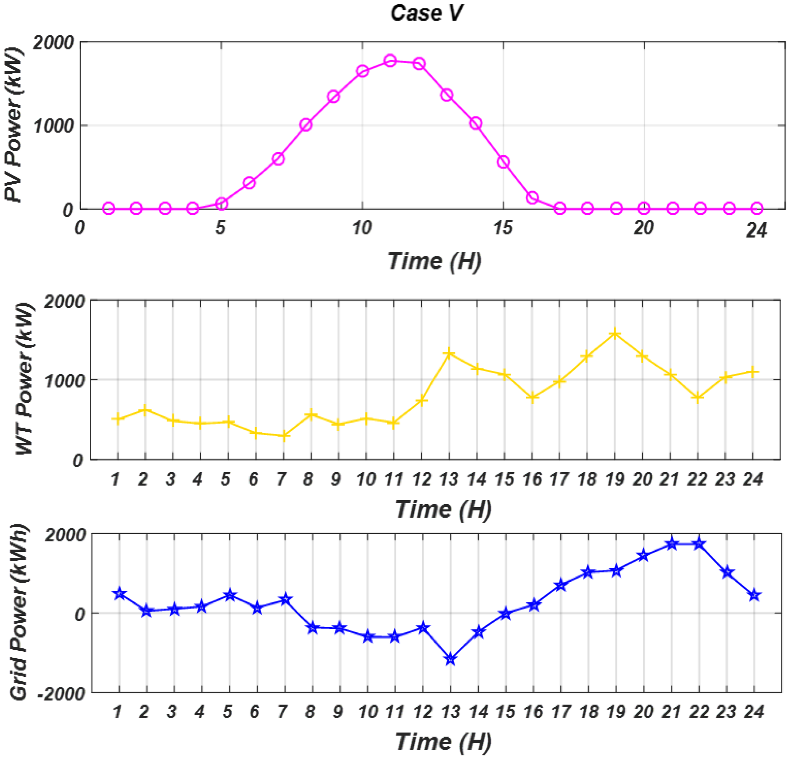
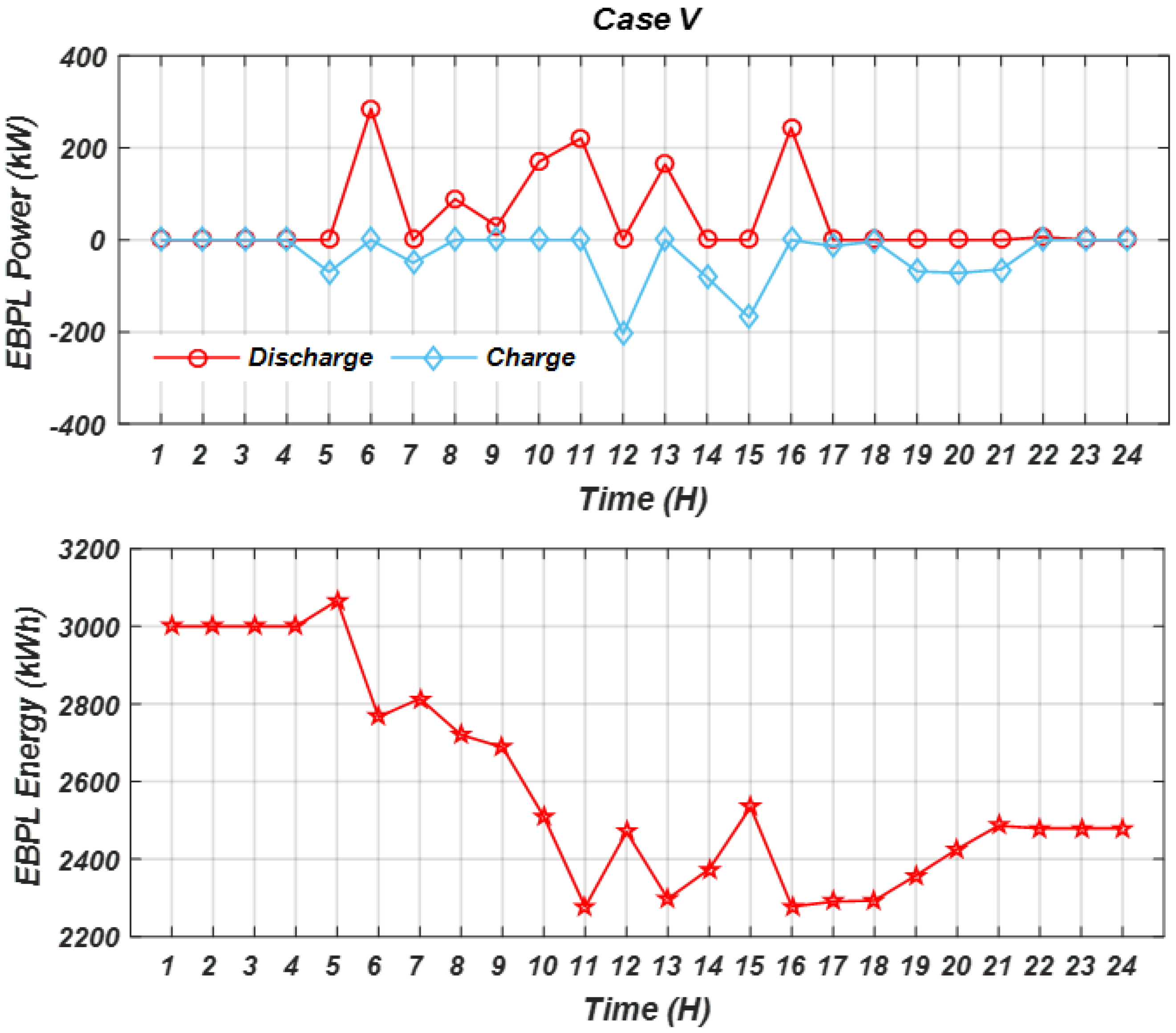
In Case V, the optimization model integrates EBPL with RES (PV and WT) under forecasted data, while renewable generation and network load uncertainties are explicitly handled using the UT–CQR method. The objective is to examine the system’s performance under both forecasted conditions and stochastic uncertainty while using EBPL for dispatch and storage. In this setup, impacts on operating costs, emission costs, energy losses, and ENS are evaluated while maintaining network reliability. Figure 19 shows the Pareto front for Case V with trade-offs among the three objectives. As in the other cases, higher operating costs are associated with higher emission costs, whereas ENS remains relatively constant. The inclusion of EBPL and stochastic modeling enhances these trade-offs, yielding more efficient and balanced solutions. Overall, the results show that using EBPL combined with uncertainty modeling improves system robustness and operational efficiency.

Figure 19. Pareto front solution set for case V (purple circles refer to the Pareto solution set).

For Case V, the system is optimized with EBPL, RES (PV, and WT), and a stochastic model that captures uncertainty in RES generation and network loading. Table 10 compares Case V with Case IV, where the system was evaluated without uncertainty. On this basis, the impact of stochastic conditions on operating cost, emission cost, energy loss, and ENS is assessed. Case V operating cost is USD 1,145,701.19, whereas Case IV is USD 1,080,464.50, an increase of 6.0%. This is driven by increased complexity of uncertainty accounting for demand and renewable generation, which requires greater flexibility and reserve capacity for both EBPL and the grid. Case V emission cost is USD 2,567,426,669.36, whereas Case IV is USD 2,443,940,919.89, a 5.1% increase. This suggests stochastic conditions lead to greater variability in renewable generation and utilization, and thus greater dependence on grid power and emissions. ENS also increases from 32.36 MWh for Case IV to 34.93 MWh for Case V, an 8.0% increase, suggesting the added challenge of load serving under variable operating conditions. While EBPL mitigates some of this volatility, the stochastic model results in a slightly higher shortfall. The energy-loss cost is USD 39,422.04 in Case V, compared with USD 37,231.87 in Case IV, representing an increase of 5.5%. This additional loss is attributable to greater swings in grid and EBPL operation under uncertain conditions.

Table 10. Optimization results for case V.

Item/Value	Base Network	Case IV	Case V
PV Size (kW)/@Site (Bus)	--	1966.49/@5	2000/@5
WT Size (kW)/@Site (Bus)	--	1668.53/@9	1785.36/@9
EBPL Size (kW)/@Site (Bus)	--	3235.23/@16	3466.08/@28
Operating Cost (USD)	--	1,080,464.50	1,145,701.19
Emission Cost (USD)	822,276,015.03	244,394,019.89	256,742,669.36
Energy Not Supplied (kWh)	58.74	32.36	34.93
Energy Loss Cost (USD)	96,732.12	37,231.87	39,422.037
PV Cost (USD)	--	213,150.00	219,150.00
WT Cost (USD)	--	656,686.10	692,370.51
EBPL Charge Cost (USD)	--	62,007.44	65,714.18
EBPL Discharge Cost (USD)	--	41,698.82	44,260.89

In component costs, Case V’s PV cost is USD 219,150.00 compared to Case IV’s USD 213,150.00, an increase of about 2.8%. This reflects the optimization of larger PV capacity for addressing uncertainty in generation. The WT cost increases by 5.4%, from Case IV’s USD 656,686.10 to Case V’s USD 692,370.51, due to the need for larger installed capacity for managing wind variability. EBPL charging cost rises from USD 62,007.44 in Case IV to USD 65,714.18 in Case V, an increase of 6.0%, as a result of increased charging cycles required for uncertainty management. Similarly, EBPL discharging cost rises from USD 41,698.82 to USD 44,260.89, an increase of 6.2%, as higher discharge activity is required to offset demand–supply discrepancies under uncertainty.

The energy supplied into the distribution system by RES, and the grid over a period of 24 h in Case V is given in Figure 20.

Figure 20. Power injected to distribution network by the PV (purple), WT (orange), and grid (blue) for Case V.

The first subplot shows PV output, which follows the typical solar generation profile, peaking at noon and decreasing toward the evening, as shown in Figure 20. The second subplot shows WT output, which varies throughout the day with wind conditions and peaks around 1000 kW. The third subplot shows grid power, which compensates for deficits when PV and WT generation is minimal. This demonstrates the role of EBPL and RES in minimizing grid dependency by storing excess energy during peak renewable generation and offsetting grid use during those periods.

Figure 21 shows the EBPL charging–discharging trend and the stored-energy profile over a 24 h period. The first subfigure presents discharging power (blue) and charging power (red), showing that the EBPL absorbs energy when renewable output exceeds demand and supplies energy when the grid requires additional support. The second subfigure shows stored-energy levels, which rise during periods of surplus RES production and decrease when energy is supplied to the grid. The optimization framework ensures that the EBPL responds smoothly to supply–demand variations while minimizing reliance on grid power.

Figure 21. The EBPL charge and discharge power as well as its energy changes (red) during a day for Case V.

3.6. Comparison of the Scenarios Results

The results of different cases are analyzed systematically in Table 11 to assess the effects of different strategies in the study. Specifically, four analyses are conducted: the effect of the implementation of EBPL (Cases I vs. II), the effect of DR (Cases II vs. III), the effect of using forecasted data (Cases III vs. IV), and the effect of using a stochastic model (Cases IV vs. V). Each comparison focuses on how these factors impact the three overall objectives of the study, i.e., operating cost, ENS, and emission cost, providing a systematic basis for evaluation. Implementation of EBPLs with RES (Case I vs. II) reduces operating cost by 5.2%, emission cost by 27.4%, and ENS by 14.1%, demonstrating the significant role of EBPLs in improving economic and reliability indices. Incorporation of DR (Case II vs. III) increases operating cost by 3.8% and emission cost by 2.3%, while slightly reducing ENS. Utilizing forecast data (Case III vs. IV) reduces operating cost by a further 4.3%, emission cost by 4.5%, and ENS by 5.1%. Adding stochastic modeling (Case IV vs. V) incurs an additional 6.0% operating cost, 5.0% emission cost, and 8.0% ENS but provides a more realistic and stable model under uncertainty.

Table 11. Comparison of the scenarios results.

Item/Value	Base Network	Case I	Case II	Case III	Case IV	Case V
PV Size (kW)/@Site (Bus)	--	2000/@4	2000/@5	2000/@5	1966.49/@5	2000/@5
WT Size (kW)/@Site (Bus)	--	1596.07/@20	1605.12/@28	1600.04/@28	1668.53/@9	1785.36/@9
EBPL Size (kW)/@Site (Bus)	--	--	3115/@32	3148/@29	3235.23/@16	3466.08/@28
Operating Cost (USD)	--	1,237,651.10	1,172,889.61	1,128,894.06	1,080,464.50	1,145,701.19
Emission Cost (USD)	822,276,015.03	360,474,505.31	261,716,433.24	255,709,362.56	244,394,019.89	256,742,669.36
Energy Not Supplied (MWh)	58.74	39.63	35.08	35.21	32.36	34.93
Energy Loss Cost (USD)	96,732.12	56,768.30	37,683.897	36,597.84	37,231.87	39,422.037
PV Cost (USD)		219,150.00	219,150.00	219,150.00	213,150.00	219,150.00
WT Cost (USD)		755,072.30	716,686.22	687,793.15	656,686.10	692,370.51
EBPL Charge Cost (USD)		--	46,619.27	31,107	62,007.44	65,714.18
EBPL Discharge Cost (USD)		--	33,927.40	39,081.58	41,698.82	44,260.89

Comparative results in Table 11 show the practical effects of progressive system improvements across the examined cases. The use of RES (Case I) significantly reduces emission cost relative to the Base Network by replacing fossil generation with renewable energy. The inclusion of EBPLs (Case II–III) further lowers operating and energy-loss costs; synchronized charging and discharging level off load fluctuations and optimize energy use. Inclusion of forecasting (Case IV) improves planning accuracy, lowering ENS and operational costs further. Finally, stochastic modeling (Case V) captures real-world uncertainty, slightly increasing costs due to risk-management conservatism but improving reliability and resilience. These results together show that integrated RES–EBPL with intelligent forecasting collectively achieves a balanced reduction in emissions, energy losses, and unserved energy to enable efficient and eco-friendly operation of the distribution network.

3.6.1. Effect of EBPL Application

Between Case I (RES without EBPL) and Case II (RES with EBPL), using EBPL results in a 27.39% reduction in emission cost, reflecting the net effect of combining energy storage and dispatch to minimize grid dependency, which tends to have higher emissions. In addition, energy not supplied (ENS) improves by 11.48%, demonstrating the role of EBPL in ensuring system reliability and mitigating energy shortages. Operating cost also improves slightly by 5.23%, since EBPL optimizes energy consumption by storing excess renewable energy and releasing it when needed, thereby reducing grid dependency (see Figure 22).

Figure 22. Reduction percentage due to effect of (a) EBPL (b) DR (c) Forecasted data (d) Uncertainty based-stochastic model.

3.6.2. Effect of DR Application

In a comparison between Case II (with EBPL) and Case III (with EBPL and DR), the incorporation of DR yields a 3.75% reduction in operating cost, reflecting the benefits of redistributing peak-hour energy demand to reduce cost. Emission cost also decreases by 2.29%, since DR facilitates optimal utilization of renewable energy, thus reducing consumption of grid and fossil-fuel-based power. ENS increases by 0.37%, meaning DR minimizes cost but slightly weakens reliability; however, its effect on ENS is smaller than its impact on operating and emission cost (see Figure 22).

3.6.3. Effect of Forecasted Data Application

Comparing Case III (with real data) and Case IV (with forecasted data), using forecasted data substantially improves system performance. Operating costs decline by 4.29%, as better forecasting of renewable energy supply and load demand allows more efficient use of RES and EBPL. Similarly, emission cost also declines by 4.42%, indicating that accurate forecasting leads to more efficient use of energy, reducing reliance on high-emission sources like the grid. ENS improves by 8.09% because forecast data help manage energy supply and demand fluctuations more efficiently, resulting in fewer energy shortages and improved network reliability (Figure 22).

3.6.4. Effect of Incorporating Stochastic Model

Finally, comparing Case IV (with forecasted data) and Case V (with forecasted data and a stochastic model), the inclusion of the stochastic model increases operating cost by 6.03%, since the model accounts for uncertainties in renewable generation and load, requiring more system flexibility and backup reserve. Emission cost rises by 5.05%, reflecting the increased variability that the stochastic model introduces, which can increase grid dependence. ENS also increases by 7.94% as the stochastic model introduces additional uncertainty in energy demand and supply, making full optimization more difficult and slightly reducing reliability. These trade-offs reflect the intricacy of introducing uncertainties into the optimization process (see Figure 22).

3.7. Comparing with Conventional Stochastic Methods

The performance of the new approach is compared with conventional stochastic methods such as Monte Carlo Simulation (MCS) and the Cloud Model (CM) in Table 12 using Case V results and comparative statistics, including computational time (s) and standard deviation (%) of the final solution. The principal objectives compared among the different methods are operating cost, emission cost, and energy not supplied (ENS). The operating cost for Case V is USD 1,145,701.19, which is lower than the MCS value of USD 1,150,716.44 and the CM value of USD 1,148,701.87. This indicates that the approach developed in this paper achieves a lower operating cost of 0.4% compared with MCS and 0.3% compared with CM. This reduction supports the effectiveness of UT–CQR-based stochastic optimization in decision-making for energy distribution. The emission cost in Case V is USD 2,567,426,669.36, which is marginally lower than MCS at USD 2,585,227,795.10, and CM at USD 2,581,354,94.36. The proposed method yields savings of 0.7% and 0.5% in emission costs over the other methods, respectively. This indicates that the advanced stochastic method effectively reduces emissions by maximizing energy-storage utilization and renewable generation, thereby reducing reliance on grid power and fossil-fuel energy. The ENS of Case V is 34.93 MWh and closely matches values calculated using MCS (35.04 MWh) and CM (35.13 MWh). The proposed method improves ENS by 0.3% and 0.6% compared to MCS and CM, respectively. This improvement demonstrates the effectiveness of UT–CQR in boosting system reliability and ensuring efficient energy distribution.

Table 12. Comparing the results of Case V with conventional stochastic methods.

Item/Value	Case V (UT–CQR)	MCS	CM
PV Size (kW)/@Site (Bus)	2000/@5	2000/@5	2000/@5
WT Size (kW)/@Site (Bus)	1785.36/@9	1794.36/@20	1770.50/@27
EBPL Size (kW)/@Site (Bus)	3466.08/@28	3457.08/@28	3579.34/@32
Operating Cost (USD)	1,145,701.19	1,150,716.44	1,148,701.87
Emission Cost (USD)	256,742,669.36	258,522,795.10	258,135,494.36
Energy Not Supplied (kWh)	34.93	35.04	35.13
Energy Loss Cost (USD)	39,422.037	395,17.81	39,496.05
PV Cost (USD)	219,150.00	219,150.00	219,150.00
WT Cost (USD)	692,370.51	694,743.88	688,802.23
EBPL Charge Cost (USD)	65,714.18	68,311.56	66,214.50
EBPL Discharge Cost (USD)	44,260.89	45,073.89	44,191.48
Computational Cost (s)	348	1953	1755
Standard Deviation (%)	0.9311	1.2853	1.19

As shown by Table 12 and Figure 23, the proposed method (Case V) completes optimization in 348 s, which is much less than MCS at 1953 s and CM at 1755 s. The heavy computational burden of MCS arises from invoking a very large number of uncertainty samples (1000 in this study). Although CM is marginally faster than MCS, it still takes substantially longer than the UT–CQR method. This confirms that the UT–CQR method proposed in this work has superior computational efficiency, even when the sampling conditions are kept identical. Moreover, as indicated in Figure 24, the standard deviation when employing UT–CQR is only 0.9311%, which is much lower than 1.2853% for MCS and 1.19% for CM, demonstrating that the proposed method yields more stable, reliable, and accurate optimization results across repeated independent runs (20 runs).

Figure 23. Computational cost comparison of Case V with MCS, and CM.

Figure 24. STD comparison of Case V with MCS, and CM.

3.8. Sensitivity Analysis

3.8.1. The Effect of EBPL Initial SOC Variations

In the Case V sensitivity analysis, the effect of varying the EBPL’s initial state of charge (SOC) on the optimization results is shown in Table 13. SOC denotes the initial charge level, with the reference SOC assumed to be 60% of maximum. The analysis examines how SOC variations impact the key objectives: operating cost, emission cost, energy-loss cost, and ENS. As SOC increases, operating cost decreases due to higher-SOC buses having the opportunity to sell power to the grid, reducing external energy purchases. Emission cost also decreases at higher SOC levels because greater stored energy reduces reliance on grid power and associated fossil-fuel emissions. Energy-loss cost likewise declines, as higher SOC enables more efficient storage and utilization. The most pronounced impact is observed on ENS. As SOC increases, ENS decreases because higher charge levels improve energy management and reduce the probability of shortages. Buses arriving with high SOC can inject energy to meet demand, improving overall reliability. In summary, the analysis confirms that higher SOC lowers operating, emission, and energy-loss costs and increases system reliability by reducing ENS. These findings underscore the importance of EBPL charge state for maximizing efficiency and reducing environmental impact.

Table 13. The results of sensitivity analysis for case V due to initial SOC variations.

Item/Value	20%	40%	60%	70%	80%	90%
Operating Cost (USD)	1,256,442.37	1,187,212.58	1,145,701.19	1,130,241.73	1,110,904.95	1,093,460.44
Emission Cost (USD)	278,932,576.621	268,487,882.003	256,742,669.36	248,523,356.29	238,982,528.62	227,195,051.14
Energy Not Supplied (MWh)	43.87	38.60	34.93	33.02	31.11	29.06
Energy Loss Cost (USD)	45,783.760	42,489.704	39,422.037	37,509.822	33,615.162	29,422.512
EBPL Charge Cost (USD)	75,440.11	69,245.49	65,714.18	62,299.90	58,194.60	53,245.97
EBPL Discharge Cost (USD)	35,383.97	40,167.45	44,260.89	47,820.86	53,906.31	59,231.91

The plots from the sensitivity analysis in Figure 25 further confirm these trends. The first plot illustrates a clear decrease in operating costs as SOC increases, validating that greater charge levels enable improved energy control. The emission cost also decreases with SOC, indicating less reliance on grid power and a cleaner energy profile. The energy-loss cost likewise decreases as SOC increases. Finally, the ENS plot shows a dramatic decline with a rise in SOC, confirming that a higher initial charge leads to fewer energy shortages. Thus, the sensitivity analysis confirms that the initial charge state of the EBPL is one of the most important optimization parameters for operating expenses, emissions, and overall system reliability.

Figure 25. The effect of EBPL SOC changes on (a) operating cost, (b) emission cost, (c) ENS, and (d) energy loss cost.

Figure 26 shows how EBPL charging and discharging costs vary with initial SOC. As SOC increases from 20% to 90%, the charging cost decreases significantly from about USD 75,440.11 to USD 53,245.97 due to reduced charging needs. Conversely, the discharging cost rises from USD 35,383.97 to over USD 59,231.91 as discharging events become more frequent with higher stored energy. This indicates a trade-off: higher SOC reduces charging expense but raises discharging expense, highlighting the importance of SOC-balance optimization to achieve optimal EBPL performance and value. Furthermore, higher initial SOC lowers the need for charging at the lot and increases discharging activity.

Figure 26. Parking charging and discharging cost process according to EBPL SOC changes.

3.8.2. The Effect of EBPL Capacity Variations

In this part, the effect of EBPL capacity variation is investigated for multiple objectives using Table 14. It follows from Table 14 that the sensitivity analysis characterizes system performance under variations in EBPL capacity in Case V. Increasing EBPL capacity from 2.5 MWh to 3.5 MWh (the case value for Case V) leads to considerable improvements in all performance measures. Specifically, operating cost decreases from USD 1,156,415.31 to USD 1,145,701.19, emission cost decreases from USD 265.13 million to USD 256.74 million, and energy not supplied (ENS) decreases from 37.18 MWh to 34.93 MWh, reflecting better system reliability. The energy-loss cost also declines slightly with capacity enhancement. However, with increased capacity above 3.5 MWh (to 4.0 MWh), incremental benefits diminish, illustrating the point of diminishing returns where increased storage yields little extra economic or reliability benefit. The results confirm that an appropriately sized EBPL can effectively balance system cost, emissions, and reliability at an optimal capacity, whereas oversizing yields minimal additional benefit and is uneconomical.

Table 14. The results of sensitivity analysis for Case V due to EBPL capacity variations.

Item/Value	2.5 MWh	3.0 MWh	3.5 MWh	4.0%
Operating Cost (USD)	1,156,415.31	1,148,912.46	1,145,701.19	1,145,682.53
Emission Cost (USD)	265,127,519.442	258,369,115.27	256,742,669.36	256,740,275.28
Energy Not Supplied (MWh)	37.18	35.12	34.93	34.93
Energy Loss Cost (USD)	41,928.61	39,835.267	39,422.037	39,420.816
EBPL Charge Cost (USD)	59,472.32	63,211.47	65,714.18	65,717.26
EBPL Discharge Cost (USD)	38,625.08	42,289.16	44,260.89	44,262.31

4. Conclusions

In this paper, a carbon-emission- and reliability-conscious stochastic optimization model for EBPL with PV and WT resources integrated into a radial 85-bus distribution network was proposed. A multi-objective optimization problem was formulated to minimize operating cost, emission cost, ENS, and energy-loss cost, and it was solved using a new MO-ESCHO. A hybrid forecasting model combining MO-ESCHO and ANN was also developed to predict renewable generation and network load. The model was tested across five scenarios involving EBPLs, DR, forecasted data, and stochastic uncertainty. The main results are as follows:

−

Implementing EBPLs with RES (Case I vs. II) reduced operating cost by 5.23%, emission cost by 27.39%, and ENS by 11.48%, demonstrating the significant role of EBPLs in improving economic and reliability indices. Incorporating DR (Case II vs. III) increased operating cost by 3.75% and emission cost by 2.29%, while slightly reducing ENS by 0.37%. Using forecasted data (Case III vs. IV) further reduced operating cost by 4.29%, emission cost by 4.42%, and ENS by 8.09%. Adding stochastic modeling (Case IV vs. V) increased operating cost by 6.03%, emission cost by 5.05%, and ENS by 7.94%, but yielded a more realistic and stable model under uncertainty.

−

The proposed MO-ESCHO outperformed MO-SCHO, MO-PSO, and MO-SCA in convergence rate, Pareto-front distribution, and diversity metrics (Hypervolume and Spacing), consistently achieving a better balance among objectives without premature convergence.

−

Compared with conventional stochastic approaches, the UT–CQR hybrid achieved higher accuracy with substantially reduced computational time (348 s vs. 1953 s for Monte Carlo and 1755 s for the Cloud Model) while maintaining stability across multiple experiments. It also yielded lower output variance over 20 independent runs (0.93% vs. 1.29% and 1.19%), demonstrating robustness under uncertainty. By integrating the Cubature Quadrature Rule into the Unscented Transformation, the hybrid approach required fewer evaluation points, mitigated the curse of dimensionality, and provided precise statistical estimates. These strengths support its superiority for real-time operation of distribution networks, where efficiency and reliability are crucial.

−

Despite these promising results, the model was tested on an 85-bus system and focused on PV, WT, and EBPLs. Future work should extend the framework to larger real distribution networks, consider additional sources of uncertainty such as market-price variations, and test the method in industrial-scale EBPL deployments. Potential industrial applications include optimal EBPL planning for smart cities, emission-mitigation strategies for public transport, and demand-side management integration in renewable-rich grids.

Appendix A.1. Conventional Sinh–Cosh Optimizer (SCHO)

Hyperbolic functions like Sinh and Cosh are widely applied in optimization. They are incorporated into the Sinh–Cosh Optimizer (SCHO) to improve exploitation. There are three stages in the optimization process: initial search, intensive exploration within promising regions, and bounded search to enforce exploration limits. The algorithm achieves faster convergence to high-quality solutions with reduced computational cost by using these mapped hyperbolic functions. The classical SCHO mathematical model is provided in detail in [33].

Appendix A.2. The Enhanced SCHO (ESCHO) Based on Entropy-Guided Exploration Control

In classical SCHO, although the structure of hyperbolic functions balances exploration and exploitation, there are limitations when optimizing complex and large-scale problems. In other words, SCHO is prone to premature convergence when search agents become clustered too early around suboptimal areas, leading to a loss of population diversity. Additionally, as the problem scale increases, the efficacy of conventional SCHO in maintaining exploration in large search spaces decreases, lowering robustness in escaping local minima. To resolve these shortcomings, we introduce an enhanced version of SCHO (ESCHO) with Entropy-Guided Exploration Control. The entropy of the population distribution is employed for adaptive control of exploration strength. Large entropy indicates sufficient diversity and allows a more intense exploitation phase, while small entropy indicates premature convergence and triggers the need for greater exploration. The adaptive entropy-guided strategy prevents premature stagnation, preserves population diversity, and increases global search capability, making convergence more predictable for complex optimization instances.

• Population Entropy

To quantify the diversity of populations, entropy is employed as a statistical measure of disorder or uncertainty. In the context of metaheuristic optimization, entropy indicates whether the population remains well dispersed in the search space or is prematurely converging to a limited region.

$$H(t)=-\sum _{i=1}^N{p}_i(t)\mathit{log}(p_i(t))$$

(A1)

where N is the population size, and p_i(t) is the normalized fitness probability of solution i at iteration t. The larger H(t) signifies more population diversity, and the smaller H(t) represents the population clustered around a small region, which raises the population trapped in local optima.

• Entropy-Guided Exploration Coefficient

To adaptively control the balance between exploration and exploitation, an entropy-guided coefficient is introduced as follows:

$$\lambda (t)={\lambda }_{\min }+({\lambda }_{\max }-{\lambda }_{\min })\cdot {\displaystyle \frac{H(t)}{H_{\max }}},$$

(A2)

where λ_min is the minimum exploration intensity, ensuring a nonzero level of exploration; λ_max is the maximum exploration intensity, applied when the population has maximum diversity; and H_max is the theoretical maximum entropy (achieved when all probabilities $p_i$ are equal).

So, when entropy is high (H(t) → H_max), λ(t) is high, which makes the algorithm do more exploitation. When entropy decreases (H(t) → 0), λ(t) falls, forcing more exploration to recover diversity.

• Position Update Rule with Entropy Control

The SCHO’s original position update rule, which uses hyperbolic functions, is adapted by adding the entropy-based coefficient as follows:

$$x_{i,j}^{t+1}=x_{i,j}^t\cdot \mathit{cosh}(\lambda (t)\cdot r_1)+X_j^{best}\cdot \mathit{sinh}(\lambda (t)\cdot r_2)$$

(A3)

where $x_{i,j}^t$ is the position of agent i in dimension j at iteration t, $X_j^{Best}$ is the current best solution in dimension j, r1, r₂∼U(0,1) are uniformly distributed random numbers. The hyperbolic functions cosh and sinh maintain SCHO’s original exploration–exploitation behavior.

With the inclusion of λ(t), the search intensity is no longer fixed but is caused to vary dynamically according to the population entropy, thus increasing immunity against premature convergence.

• Diversity Recovery Mechanism

The diversity restoration mechanism is triggered when the population diversity drops below a predefined threshold value (Hth). The mechanism reinitializes a few individuals at random to prolong the search and prevent stagnation:

$$x_{ij}^{t+1}=l{b}_j+rand\left(\mathrm{0,1}\right)\cdot (u{b}_j-l{b}_j)$$

(A4)

where lb_j and ub_j are the lower and upper bounds of the search space in dimension j. This operator works in a similar manner to a mutation operator, reintroducing diversity and enhancing exploration. Also, rand(0,1) returns a scalar random sample from the continuous uniform distribution on $[0,1]$; each call yields an independent draw.

The proposed ESCHO has several significant advantages. First, the use of entropy enables adaptive control, and the algorithm can automatically trade off exploration and exploitation based on the current state of the population. Second, it avoids premature convergence, because the decline in diversity automatically triggers heightened exploration, allowing the search to escape local optima. Third, it is robust on high-dimensional problems, because entropy-based control reduces the likelihood of stagnation in large-scale and complex optimization problems. Collectively, these features make ESCHO a more resilient optimizer, able to preserve diversity, prevent premature convergence, and achieve enhanced global search performance.

Appendix A.3. Multi-Objective Optimization Approach

A fuzzy multi-objective optimization technique, MO-ESCHO, is used to solve multiple conflicting objectives under system constraints. MO-ESCHO optimizes the utilization of EBPL, PV, and wind resources in a distribution system by simultaneously minimizing operating cost, emission cost, and energy not supplied (ENS) while maximizing reliability. Since all objectives are cast in a smaller-the-better (STB) form via ENS, decreasing values indicate better performance, while the conflicting nature of objectives implies that trade-offs are necessary. By framing the problem as a multi-objective optimization, the Pareto front of optimal solutions is obtained, with balanced solutions provided without disproportionately compromising one factor for another. This ensures realistic, practical, and fair solutions, enabling the decision-maker to select the most appropriate strategy based on system needs and priorities [30,31].

$$\begin{array}{c}F\left(X\right)=\left[f_1\left(X\right),f_2\left(X\right),\dots ,f_z\left(X\right)\right]\\ \mathrm{s}.\mathrm{t}.\left\{\begin{array}{c}g\left(X\right)<0\\ h\left(X\right)=0\end{array}\right.\end{array}$$

(A5)

where X is a vector consisting of the decision variables, F(X) are the objective functions of the decision vector, g(X) are the inequality constraints, and z is the number of objectives (z = 3).

The Pareto frontier is a group of candidate solutions with various combinations of objectives, providing planners with a choice to select more than one option. Planners use their experience and professional judgment to choose the most appropriate solution from this frontier. Nevertheless, as subjective evaluations inherently involve uncertainty, a fuzzy decision-making approach is applied to determine the final solution. The focus of this fuzzy-based approach is selecting the most appropriate solution(s) among the non-dominated set, depending on decision-makers’ priorities and preferences. In most cases, every objective function is defined by a single membership function, which can be adjusted to account for the planner’s experience and preference. This membership function is then attributed to each objective with a degree of satisfaction, thus allowing a more systematic and responsive choice process. The membership function for a solution $k$ with $z$ objective functions can be mathematically established as follows [30,31]:

$${\mu }_z=\left\{\begin{array}{cc}1,& f_Z\left(X\right)\le f_Z^{\mathrm{m}\mathrm{i}\mathrm{n}}\\ {\displaystyle \frac{f_Z^{\mathrm{m}\mathrm{a}\mathrm{x}}-f_Z}{f_Z^{\mathrm{m}\mathrm{a}\mathrm{x}}-f_Z^{\mathrm{m}\mathrm{i}\mathrm{n}}}},& f_Z^{\mathrm{m}\mathrm{i}\mathrm{n}}<f_Z\left(X\right)<f_Z^{\mathrm{m}\mathrm{a}\mathrm{x}}\\ 0,& f_Z\left(X\right)\ge f_Z^{\mathrm{m}\mathrm{a}\mathrm{x}}\end{array}\right.$$

(A6)

where $f_Z^{\mathrm{m}\mathrm{i}\mathrm{n}}$ and $f_Z^{\mathrm{m}\mathrm{a}\mathrm{x}}$ are lower and upper values of the Zth objective function, respectively, and f_Z(X) represents the value of the Zth objective during optimization. The membership function operates in the interval [0, 1] where μ_z = 1 represents complete satisfaction and μ_z = 0 represents complete dissatisfaction. The degree of satisfaction μ_z thus provides a flexible and intuitive tool for ranking individual objectives. Moreover, the fuzzy membership function normalizes objectives with different units to a common range of 0 to 1. Normalization helps decision-makers compare and weigh multiple, sometimes conflicting objectives in a balanced way, thereby supporting informed and consistent decision-making.

According to [30,31], the normalization of the membership function μ_z is given by the following:

$${\mu }^k={\displaystyle \frac{\sum _{z=1}^{N_F}{\mu }_z^k}{\sum _{k=1}^{N_{ND}}\sum _{z=1}^{N_F}{\mu }_z^k}}$$

(A7)

In the definition, N_F is used to denote the number of objective functions optimized, and ND is used to denote the number of solutions on the Pareto front that cannot dominate others.

The nearer an objective function is to its maximum, the smaller its corresponding μ. When we maximize the minimum of all ${\mu }_z$ during optimization, we drive all objective functions toward their lowest achievable values. Thus, the simultaneous minimization of all objectives is achieved. The governing principle can be written as follows:

$${\mu }_D^k\left(x\right)=\mathrm{m}\mathrm{i}\mathrm{n}({\mu }_{z1}\left(x\right),{\mu }_{z2}\left(x\right),{\mu }_{z3}\left(x\right))$$

(A8)

$${\mathrm{m}\mathrm{a}\mathrm{x}(\mu }_D^k\left(x\right))$$

(A9)

where ${\mu }_D^k\left(x\right)$ denotes the membership value associated with the optimal decision function.

Appendix A.4. Implementing the MO-ESCHO

The flowchart of the proposed fuzzy multi-objective approach to optimize the EBPL and renewable PV and wind energy resources in distribution network is depicted in Figure A1. Also, pseudo-code of the MO-ESCHO is presented in Algorithm A1.

Figure A1. The multi-objective optimization flowchart to solve the problem.

Algorithm A1: Pseudo-code of the MO-ESCHO.

% Initialize MO-ESCHO parameters: ct, T, BS1, u, m, n, α, β, p, and q % Initialize entropy-control parameters: λmin, λmax, γ, and entropy threshold Hth % Initialize candidate solutions X randomly X = rand(N, dim) * (ub − lb) + lb; % Initialize objective matrix F and external archive A_ext F = zeros(N, M); A_ext = ∅; % Main optimization loop for t = 1:MaxIter  % Evaluate all objective functions  for i = 1:N   F(i,:) = evaluateMultiObjective(X(i,:)); % <-- user-defined objectives  end % Perform non-dominated sorting and compute crowding distance  [Fronts, Rank] = nonDominatedSorting(F);  CD = crowdingDistance(Fronts, F); % Calculate population entropy and update λ adaptively  pi = normalizeFitness(F);  H = -sum(pi .* log(pi + eps));  λ = λmin + (λmax − λmin) * (H/Hmax); % Select leader from the first Pareto front  X_best = selectLeader(Fronts, CD, X); for i = 1:N   for j = 1:dim    % Compute switching parameter A    A = computeA(t, MaxIter, ct, p, q); % Check for bounded search phase    if mod(t, BS1) == 0     % Reinitialize candidate within bounds     X(i,j) = lb(j) + rand() * (ub(j) − lb(j));    end % Choose phase based on A    if A > 1     % Exploration Mode (entropy-guided)     a1 = 2 − t/MaxIter;     r1 = rand(); r2 = rand();     W1 = a1 * r1 − a1;     W2 = a1 * r2;     if t <= T      % Early exploration step      X(i,j) = X(i,j) + λ * (W1 * (X_best(j) − X(i,j)) + W2 * sinh(r1));     else      % Late exploration step      epsilon = 0.003;      W2 = W2 * epsilon;      X(i,j) = X(i,j) + λ * W2;     end    else     % Exploitation Mode (entropy-guided)     a1 = 2 − t/MaxIter;     r3 = rand();     W3 = a1 * r3;     if t <= T      % First exploitation step      X(i,j) = X(i,j) + λ * (W3 * cosh(r3) * (X_best(j) − X(i,j))) + rand();     else      % Local refinement phase      X(i,j) = X(i,j) + λ * epsilon * W3;     end    end % Diversity restoration based on entropy threshold    if H < Hth     R = −1 + 2 * rand(); % R_(i,j)^t ∼ U(−1,1)     X(i,j) = X(i,j) + γ * R;    end % Bound control    X(i,j) = max(min(X(i,j), ub(j)), lb(j));   end  end % Update external archive with non-dominated solutions  A_ext = updateArchive(A_ext, X, F); % Compute fuzzy membership for final decision  μ = computeFuzzyMembership(F); end % Extract Pareto front and determine fuzzy-best compromise PF = extractParetoFront(A_ext); X_best_fuzzy = fuzzyDecision(PF, μ);

References

1. Verma, H.K.; Gupta, N.; Agrawal, P.K.; Niazi, K.R.; Swarnkar, A. EV charging strategies for office parking lots to relieve local grids. Sustain. Energy Grids Netw. 2025, 44, 101942. [Google Scholar] [CrossRef]
2. Nurmuhammed, M.; Akdağ, O.; Karadağ, T.; Kafafy, M. Multi-Factor Optimization for Electric Bus Charging Stations: Integrating Electrical, Social, and Environmental Perspectives. Energy Nexus 2025, 19, 100500. [Google Scholar] [CrossRef]
3. Yánez, A.H.; Cindy, F.G.; Yánez, E.R.; Delgado, J.C.V.; Barzola-Monteses, J. A brief review of the techniques used to locate electric bus charging stations. In Proceedings of the 2024 IEEE Eighth Ecuador Technical Chapters Meeting (ETCM), Cuenca, Ecuador, 15–18 October 2024; IEEE: New York, NY, USA, 2024; pp. 1–6. [Google Scholar]
4. Orbe, D.; Salazar, L.; Vásquez, P.; Chamorro, W.; Medina, J. Influence of Optimal Charging Station Integration on Electric Power Distribution Grid: Case of Electric Bus-Based Transport System. Eng. Proc. 2024, 77, 22. [Google Scholar]
5. Hadi Abdulwahid, A.; Al-Razgan, M.; Fakhruldeen, H.F.; Churampi Arellano, M.T.; Mrzljak, V.; Arabi Nowdeh, S.; Moghaddam, M.J.H. Stochastic multi-objective scheduling of a hybrid system in a distribution network using a mathematical optimization algorithm considering generation and demand uncertainties. Mathematics 2023, 11, 3962. [Google Scholar] [CrossRef]
6. Tong, X.; Zhao, S.; Chen, H.; Wang, X.; Liu, W.; Sun, Y.; Zhang, L. Optimal dispatch of a multi-energy complementary system containing energy storage considering the trading of carbon emission and green certificate in China. Energy 2025, 314, 134215. [Google Scholar] [CrossRef]
7. De Lima, T.D.; Cordero, L.G.; Soares, J.; Franco, J.F. Optimal probabilistic framework for grid cost operation considering voltage probability constraints and high penetration of EVs, wind and PV generation. J. Clean. Prod. 2025, 521, 146241. [Google Scholar] [CrossRef]
8. De Lima, T.D.; Franco, J.F.; Lezama, F.; Soares, J.; Vale, Z. Joint optimal allocation of electric vehicle charging stations and renewable energy sources including CO2 emissions. Energy Inform. 2021, 4 (Suppl. S2), 33. [Google Scholar] [CrossRef]
9. Ghofrani, M.; Majidi, M. A comprehensive optimization framework for EV-Renewable DG coordination. Electr. Power Syst. Res. 2021, 194, 107086. [Google Scholar] [CrossRef]
10. Veisi, M. Economic sizing and placement of hydrogen fueling and electric vehicles charging stations powered by renewable and battery systems in smart distribution network. Results Eng. 2025, 27, 106657. [Google Scholar] [CrossRef]
11. Alahyari, A.; Ehsan, M.; Mousavizadeh, M. A hybrid storage-wind virtual power plant (VPP) participation in the electricity markets: A self-scheduling optimization considering price, renewable generation, and electric vehicles uncertainties. J. Energy Storage 2019, 25, 100812. [Google Scholar] [CrossRef]
12. Yao, M.; Moradi, Z.; Pirouzi, S.; Marzband, M.; Baziar, A. Stochastic economic operation of coupling unit of flexi-renewable virtual power plant and electric spring in the smart distribution network. IEEE Access 2023, 11, 75979–75992. [Google Scholar] [CrossRef]
13. Gupta, K.; Achathuparambil Narayanankutty, R.; Sundaramoorthy, K.; Sankar, A. Optimal location identification for aggregated charging of electric vehicles in solar photovoltaic powered microgrids with reduced distribution losses. Energy Sources Part A Recovery Util. Environ. Eff. 2024, 46, 6289–6304. [Google Scholar] [CrossRef]
14. Affolabi, L.; Shahidehpour, M.; Gan, W.; Yan, M.; Chen, B.; Pandey, S.; Vukojevic, A.; Paaso, E.A.; Alabdulwahab, A.; Abusorrah, A. Optimal transactive energy trading of electric vehicle charging stations with on-site PV generation in constrained power distribution networks. IEEE Trans. Smart Grid 2021, 13, 1427–1440. [Google Scholar] [CrossRef]
15. Liu, J.; Zhong, C. An economic evaluation of the coordination between electric vehicle storage and distributed renewable energy. Energy 2019, 186, 115821. [Google Scholar] [CrossRef]
16. Turan, M.T.; Ates, Y.; Erdinc, O.; Gokalp, E.; Catalão, J.P. Effect of electric vehicle parking lots equipped with roof mounted photovoltaic panels on the distribution network. Int. J. Electr. Power Energy Syst. 2019, 109, 283–289. [Google Scholar] [CrossRef]
17. Nasab, M.A.; Al-Shibli, W.K.; Zand, M.; Ehsan-Maleki, B.; Padmanaban, S. Charging management of electric vehicles with the presence of renewable resources. Renew. Energy Focus 2024, 48, 100536. [Google Scholar] [CrossRef]
18. Almazroui, A.; Mohagheghi, S. Coordinated Control of Photovoltaic Resources and Electric Vehicles in a Power Distribution System to Balance Technical, Environmental, and Energy Justice Objectives. Processes 2025, 13, 1979. [Google Scholar] [CrossRef]
19. Bonela, R.; Roy Ghatak, S.; Swain, S.C.; Lopes, F.; Nandi, S.; Sannigrahi, S.; Acharjee, P. Analysis of Techno–Economic and Social Impacts of Electric Vehicle Charging Ecosystem in the Distribution Network Integrated with Solar DG and DSTATCOM. Energies 2025, 18, 363. [Google Scholar] [CrossRef]
20. Al-Sahlawi, A.A.K.; Ayob, S.M.; Tan, C.W.; Ridha, H.M.; Hachim, D.M. Optimal design of grid-connected hybrid renewable energy system considering electric vehicle station using improved multi-objective optimization: Techno-economic perspectives. Sustainability 2024, 16, 2491. [Google Scholar] [CrossRef]
21. Nareshkumar, K.; Das, D. Optimal location and sizing of electric vehicles charging stations and renewable sources in a coupled transportation-power distribution network. Renew. Sustain. Energy Rev. 2024, 203, 114767. [Google Scholar] [CrossRef]
22. Zangmo, R.; Sudabattula, S.K.; Mishra, S.; Dharavat, N.; Golla, N.K.; Sharma, N.K.; Jadoun, V.K. Optimal placement of renewable distributed generators and electric vehicles using multi-population evolution whale optimization algorithm. Sci. Rep. 2024, 14, 28447. [Google Scholar] [CrossRef] [PubMed]
23. Veisi, M. Stochastic economic placement and sizing of electric vehicles charging station with renewable units and battery bank in smart distribution network. Sci. Rep. 2025, 15, 24235. [Google Scholar] [CrossRef]
24. Zhang, J.; Wang, S.; Zhang, C.; Luo, F.; Dong, Z.Y.; Li, Y. Planning of electric vehicle charging stations and distribution system with highly renewable penetrations. IET Electr. Syst. Transp. 2021, 11, 256–268. [Google Scholar] [CrossRef]
25. Alam, M.J.E.; Muttaqi, K.M.; Sutanto, D. Effective utilization of available PEV battery capacity for mitigation of solar PV impact and grid support with integrated V2G functionality. IEEE Trans. Smart Grid 2015, 7, 1562–1571. [Google Scholar] [CrossRef]
26. Haji-Aghajani, E.; Hasanzadeh, S.; Heydarian-Forushani, E. A novel framework for planning of EV parking lots in distribution networks with high PV penetration. Electr. Power Syst. Res. 2023, 217, 109156. [Google Scholar] [CrossRef]
27. Kumar, R.; Singh, S.; Bilga, P.S.; Jatin; Singh, J.; Singh, S.; Scutaru, M.-L.; Pruncu, C.I. Revealing the benefits of entropy weights method for multi-objective optimization in machining operations: A critical review. J. Mater. Res. Technol. 2021, 10, 1471–1492. [Google Scholar] [CrossRef]
28. Davoudkhani, I.F.; Zishan, F.; Mansouri, S.; Abdollahpour, F.; Grisales-Noreña, L.F.; Montoya, O.D. Allocation of renewable energy resources in distribution systems while considering the uncertainty of wind and solar resources via the multi-objective Salp Swarm algorithm. Energies 2023, 16, 474. [Google Scholar] [CrossRef]
29. Kalantari, A.; Lesani, H. Operation Scheduling of Distribution Network with Photovoltaic/Wind/Battery Multi-Microgrids and Reconfiguration considering Reliability and Self-Healing. Int. J. Energy Res. 2024, 2024, 5724653. [Google Scholar] [CrossRef]
30. Nowdeh, S.A.; Davoudkhani, I.F.; Moghaddam, M.H.; Najmi, E.S.; Abdelaziz, A.Y.; Ahmadi, A.; Razavi, S.; Gandoman, F.H. Fuzzy multi-objective placement of renewable energy sources in distribution system with objective of loss re-duction and reliability improvement using a novel hybrid method. Appl. Soft Comput. 2019, 77, 761–779. [Google Scholar] [CrossRef]
31. Shayeghi, H.; Davoudkhani, I.F. Uncertainty aware energy management in microgrids with integrated electric bicycle charging stations and green certificate market. Sci. Rep. 2025, 15, 26374. [Google Scholar] [CrossRef]
32. Habibi, S.; Effatnejad, R.; Hedayati, M.; Hajihosseini, P. Stochastic energy management of a microgrid incorporating two-point estimation method, mobile storage, and fuzzy multi-objective enhanced grey wolf optimizer. Sci. Rep. 2024, 14, 1667. [Google Scholar]
33. Bai, J.; Li, Y.; Zheng, M.; Khatir, S.; Benaissa, B.; Abualigah, L.; Wahab, M.A. A sinh cosh optimizer. Knowl.-Based Syst. 2023, 282, 111081.F. [Google Scholar] [CrossRef]
34. Lei, H.; Guo, Y.; Khan, N. Forecasting energy use and efficiency in transportation: Predictive scenarios from ANN models. Int. J. Hydrogen Energy 2025, 106, 1373–1384. [Google Scholar] [CrossRef]
35. Pereira, S.; Canhoto, P.; Salgado, R. Development and assessment of artificial neural network models for direct normal solar irradiance forecasting using operational numerical weather prediction data. Energy AI 2024, 15, 100314. [Google Scholar] [CrossRef]
36. NASA Remote Sensing Validation Data: Saudi Arabia. Available online: https://www.nrel.gov/grid/solar-resource/saudi-arabia (accessed on 25 February 2025).
37. Hai, T.; Singh, N.S.S.; Jamal, F. Energy management of a microgrid with integration of renewable energy sources considering energy storage systems with electricity price. J. Energy Storage 2025, 110, 115191. [Google Scholar] [CrossRef]
38. Butler, Q.; Ziada, Y.; Gadsden, S.A. Gaussian Filtering using a Spherical-Radial Double Exponential Cubature. IEEE Open J. Signal Process. 2025, 6, 1056–1076. [Google Scholar] [CrossRef]
39. Prakash, D.B.; Lakshminarayana, C. Optimal siting of capacitors in radial distribution network using whale optimization algorithm. Alex. Eng. J. 2017, 56, 499–509. [Google Scholar] [CrossRef]
40. Fathy, A.; Abdelaziz, A.Y. Competition over resource optimization algorithm for optimal allocating and sizing parking lots in radial distribution network. J. Clean. Prod. 2020, 264, 121397. [Google Scholar] [CrossRef]
41. Billinton, R.; Allan, R.N. Reliability Assessment of Large Electric Power Systems; Springer Science & Business Media: New York, NY, USA, 2012. [Google Scholar]
42. Kennedy, J.; Eberhart, R. Particle swarm optimization. In Proceedings of the ICNN’95—International Conference on Neural Networks, Perth, Australia, 27 November–1 December 1995; IEEE: New York, NY, USA, 1995; Volume 4, pp. 1942–1948. [Google Scholar]
43. Mirjalili, S. SCA: A sine cosine algorithm for solving optimization problems. Knowl.-Based Syst. 2016, 96, 120–133. [Google Scholar] [CrossRef]
Disclaimer/Publisher’s Note: The statements, opinions and data contained in all publications are solely those of the individual author(s) and contributor(s) and not of MDPI and/or the editor(s). MDPI and/or the editor(s) disclaim responsibility for any injury to people or property resulting from any ideas, methods, instructions or products referred to in the content.
Article Metrics
Citations
Article Access Statistics
Multiple requests from the same IP address are counted as one view.