Digital Implementation of LCC Resonant Converters for X-ray Generator with Optimal Trajectory Startup Control

Abstract

High voltage LCC resonant converters have been widely used in X-ray imaging systems in automobile nondestructive testing (NDT) applications. Low ripple voltage waveforms with fast-rising time under no-overshoot response are required for safety in such applications. The optimal state trajectory control (OTC) based on the state plane model is one of the most effective control methods to optimize transient response. Dynamic variations of the resonant voltages/currents are described as corresponding trajectories on the state plane. The transient relations can be determined by evaluating the geometric relationships of the trajectories. However, the LCC resonant converter has more state variables, resulting in more complex calculations that make the state trajectory control challenging. Furthermore, the startup duration is the most demanding process of the state trajectory control. In this paper, a digital implementation based on a hybrid controller built in a field-programmable gate array (FPGA) is proposed for LCC resonant converters with optimal trajectory startup control. A coordinated linear compensator is employed to control the switching frequency during steady-state conditions, hence eliminating the steady-state error. The experimental results were conducted on a 140-kV/42-kW LCC resonant converter for an X-ray generator. It achieves a short rising time of output voltage with no additional current or voltage stress in the resonant tank during startup compared to the conventional digital implementation control.

1. Introduction

Effective detection and identification must be carried out to ensure the product quality of the automobile hub. Nondestructive testing technology (NDT) plays an essential role in improving product quality and production efficiency. At the same time, it is one of the most effective testing methods in testing technology. X-ray imaging technology is widely used in nondestructive testing because of its intuitive and accurate test results [1]. Due to the high quality of X-ray imaging, it can accurately provide real information about automobile hub defects. Therefore, the digital image of the wheel hub can be obtained through the X-ray imaging system.

The X-ray generator is a device that supplies electric power to the X-ray tube and permits the selection of X-ray energy (voltage), X-ray quantity (current), and exposure time. The generator has three main interrelated electric circuits to serve three main functions: (1) The power supply for heating the cathode filament and evaporating electrons is provided by the filament circuit; (2) the high-voltage circuits are used to increase the speed of electrons from the cathode to the anode to produce X-rays; (3) the timer circuit (exposure timer) controls the duration of X-ray. Figure 1 shows a block diagram of a typical X-ray generator [2]. The X-ray tube application presented in this paper utilizes an Input Single Output Series (ISOS) LCC resonant converter [3], as illustrated in Figure 2, which features a multilevel series arrangement with diode rectified output capacitors [4], increasing flexibility and scalability.

Figure 1. Block diagram of an X-ray generator.

Figure 2. The topology of LCC resonant converter.

Researchers have proposed various modeling methods to operate resonant converters properly. Fundamental harmonic approximation (FHA) is widely utilized, but the ignorance of harmonic components reduces the accuracy of circuit analysis [5]. Extended describing function (EDF) modeling methods [6] or time-domain analysis methods [7] are adopted to solve such problems. A state trajectory analysis was proposed to achieve higher accuracy of resonant tank behavior control [8]. The resonant process was analyzed in the state plane, and the analytical formula can be obtained based on geometric relationships of the trajectory [9]. For series resonant converter (SRC), parallel resonant converter (PRC), and LLC resonant converters [10], state trajectory analysis and control have been applied in addressing unpredictable dynamics, burst mode for light load [11], soft startup, and short circuit protection [12]. However, more state variables make it more complicated for LCC resonant converters to present their relationships in a 2-D plane coordinate system. Therefore, it is very challenging to implement the state trajectory control. Furthermore, the startup duration is the toughest process of the state trajectory control [13].

This article proposes a state trajectory startup control and real-time implementation for ISOS Type LCC resonant converters with a capacitive output filter in a 140 kV/42 kW X-ray generator. The state trajectory startup control for LCC converter is optimized and conducted using FPGA to achieve low ripple voltage waveforms with fast-rising time under no-overshoot response. Furthermore, the state trajectory-based startup is successfully applied to an industry-level X-ray generator with a Power/ Voltage Level of 42 kw/140 kV for the first time. The rest of the paper is organized as follows. Section 2 introduces the state plane analysis method and state trajectory, including six operation conditions in detail, and describes the optimal trajectory control method for the soft startup process. Section 3 introduces the implementation of the state trajectory control in FPGA. Finally, the experimental results on a 140 kV/42 kW HV power supply used for the X-ray generator are presented to verify the proposed model and control strategy.

2. Analysis of State Trajectory-Based Startup for LCC Converter

The control mechanism for the LCC converter’s state trajectory-based startup is depicted in Figure 3. The figure illustrates the topology of the LCC converter and the sampling and control processes used by the control system. The state trajectory-based startup for the LCC converter is divided into three stages [14].

Figure 3. Block diagram of Hybrid control for LCC resonant converter.

In Stage 1, the resonant current of the LCC converter rises to −i_maxN in the first switching cycle. ±i_maxN is the limit value of the resonant current in the state trajectory control, as shown in Figure 4. At the end of converter startup, the frequency value compensated by PI control is added to the frequency value predicted by state trajectory control [15]. V_in and V_o are sampled for the calculation of state trajectory control. As described in Figure 4, the LCC converter works in the 3rd operating mode with S1 and S4. In the 3rd operating mode, the state trajectory is arc AB, and the state trajectory equation is given as:

$$i_{\mathrm{LrN}}^2(t)+{\left[V_{\mathrm{CprN}}(t)-1\right]}^2=i_{\mathrm{LrN}}^2(t_2)+{\left[V_{\mathrm{CprN}}(t_2)-1\right]}^2$$

(1)

where, i_LrN(t) is the normalized resonant current value, V_CrN(t) is the normalized voltage value of capacitor C_r, V_CpN(t) is the normalized voltage value of capacitor C_p, V_CprN(t) is the sum of V_CrN(t) and V_CpN(t). i_LrN(t₂) and V_CprN(t₂) are the initial values of i_LrN(t) and V_CprN(t) in the 3rd operating mode.

Figure 4. Initial trajectory of startup.

Then, the LCC converter operates in the 6th operating mode with S2 and S3, and the state trajectory is arc BCD. The state trajectory of the 6th operating mode is given as:

$$i_{\mathrm{LrN}}^2(t)+{\left[V_{\mathrm{CprN}}(t)+1\right]}^2=i_{\mathrm{LrN}}^2(t_5)+{\left[V_{\mathrm{CprN}}(t_5)+1\right]}^2$$

(2)

where, i_LrN(t₅) and V_CprN(t₅) are the initial values of i_LrN(t) and V_CprN(t) in the 6th operating mode.

The arc radius of the state trajectories in the 3rd operating mode and the 6th operating mode are defined as ρ_T0 and ρ_T1. The central angle of arc AB is defined as θ₀, and the central angle of arc BCD is defined as θ₁ + θ₂. The process of solving the central angle can be obtained as:

$$\{\begin{array}{l}{\theta }_0=\arccos \left(\frac{{\rho }_{T_0}^2+2^2-{\rho }_{T_1}^2}{2·2·{\rho }_{T_0}}\right)\\ {\theta }_1=\arccos \left(\frac{{\rho }_{T_1}^2+2^2-{\rho }_{T_0}^2}{2·2·{\rho }_{T_1}}\right)\\ {\theta }_2=\arcsin \left(\frac{i_{\max \mathrm{N}}}{{\rho }_{T_0}}\right)\end{array}$$

(3)

According to Figure 4. ρ_T0 and ρ_T1 can be expressed as:

$$\begin{array}{l}{\rho }_{T_0}=1\\ {\rho }_{T_1}^2=i^2{}_{\mathrm{maxN}}+1\end{array}$$

(4)

Therefore, the conduction time T₀ of S₁ and S₄ and T₁ of S₂ and S₃ can be derived as:

$$\begin{array}{l}{T}_0=\frac{{\theta }_0}{{\omega }_0}\\ T_1=\frac{{\theta }_1+{\theta }_2}{{\omega }_0}\end{array}$$

(5)

In stage 2, the maximum values of resonant current are kept constant [16]. The energy in the resonator increases rapidly and is transmitted to the load. The output voltage of LCC converter rises quickly. The power in the resonator is low, and the resonant current value reaches the maximum at the switching time [17].

As shown in Figure 5, the state trajectory of the whole cycle is defined as 6 operating modes. In the 1st operating mode, the center coordinates of the state trajectory arc are (1, 0), and the radius is R [18]. In the 2nd operating mode, the state trajectory is an ellipse. In the 3rd operating mode, the state trajectory equation is the same as in stage 1. The trajectory equation of Mode I-III is given as:

$$i_{\mathrm{LrN}}^2(t)+{\left[V_{\mathrm{CprN}}(t)-1\right]}^2=i_{\mathrm{LrN}}^2(t_0)+{\left[V_{\mathrm{CprN}}(t_0)-1\right]}^2$$

(6)

$${\left(\frac{i_{\mathrm{LrN}}(t)}{Z_0/Z_1}\right)}^2+{\left[V_{\mathrm{CprN}}(t)-1\right]}^2={\left(\frac{i_{\mathrm{LrN}}(t_1)}{Z_0/Z_1}\right)}^2+{\left(V_{\mathrm{CprN}}(t_1)-1\right)}^2$$

(7)

$$i_{\mathrm{LrN}}^2(t)+{\left[V_{\mathrm{CprN}}(t)-1\right]}^2=i_{\mathrm{LrN}}^2(t_2)+{\left[V_{\mathrm{CprN}}(t_2)-1\right]}^2$$

(8)

where, Z₀ is the double-element resonance impedance [19], Z₁ is the triple-element resonance impedance, i_LrN(t₀) and V_CprN(t₀) are the initial values of i_LrN(t) and V_CprN(t) in the 1st operating mode, i_LrN(t₁) and V_CprN(t₁) are the initial values of i_LrN(t) and V_CprN(t) in the 2nd operating mode.

Figure 5. State Trajectory of LCC resonant converter stage 2.

Similarly, according to the geometric symmetry of the trajectory, the trajectory equation of Mode IV–VI can be obtained as:

$$i_{\mathrm{LrN}}^2(t)+{\left[V_{\mathrm{CprN}}(t)+1\right]}^2=i_{\mathrm{LrN}}^2(t_3)+{\left[V_{\mathrm{CprN}}(t_3)+1\right]}^2$$

(9)

$${\left(\frac{i_{\mathrm{LrN}}(t)}{Z_0/Z_1}\right)}^2+{\left[V_{\mathrm{CprN}}(t)+1\right]}^2={\left(\frac{i_{\mathrm{LrN}}(t_4)}{Z_0/Z_1}\right)}^2+{\left(V_{\mathrm{CprN}}(t_4)+1\right)}^2$$

(10)

$$i_{\mathrm{LrN}}^2(t)+{\left[V_{\mathrm{CprN}}(t)+1\right]}^2=i_{\mathrm{LrN}}^2(t_5)+{\left[V_{\mathrm{CprN}}(t_5)+1\right]}^2$$

(11)

where, i_LrN(t₃) and V_CprN(t₃) are the initial values of i_LrN(t) and V_CprN(t) in the 4th operating mode, i_LrN(t₄) and V_CprN(t₄) are the initial values of i_LrN(t) and V_CprN(t) in the 5th operating mode.

The coordinates of points A, B, C, D are substituted into the state trajectory equation, and the equation can be rewritten as:

$$\{\begin{array}{l}(V_B+1{)}^2+(\frac{I_B}{Z_0/Z_1}{)}^2=R^2\\ (V_B-1{)}^2+I_B^2=r^2\\ (V_C-1{)}^2+I_C^2=r^2\\ (V_C+1{)}^2+I_C^2=R^2\\ V_D+1=R\\ -V_A+1=R\\ V_D=-V_A\\ I_C=i_{\max \mathrm{N}}\end{array}$$

(12)

where, V_A is the value of V_CprN(t) at point A, V_B is the value of V_CprN(t) at point B, V_C is the value of V_CprN(t) at point C, V_D is the value of V_CprN(t) at point D, R is the radius of state trajectory arc in the 3rd operating mode, r is the radius of state trajectory arc in the 4th operating mode.

Through the analysis of the state trajectory in stage 2, and (12) can be simplified as:

$$\{\begin{array}{l}{V}_A=\frac{-\left(B_1{C}_1+1\right)+\sqrt{(B_1{C}_1+1{)}^2-\left(B_1{}^2-1\right)\left(C_1{}^2+i_{\max \mathrm{N}}^2-1\right)}}{B_1{}^2-1}\hfill \\ V_D=B_1{V}_A+C_1+1\hfill \\ V_B=V_A+A_1+1\hfill \\ R=1-V_A\hfill \\ r=\sqrt{(V_D-1{)}^2+i_{\max \mathrm{N}}^2}\hfill \end{array}$$

(13)

The parameters A₁, B₁, and C₁ can be expressed as (14).

$$A_1=\frac{2V_o{C}_p}{n{V}_{in}}(\frac{1}{C_p}+\frac{1}{C_r})-1 B_1=(1-(\frac{Z_0}{Z_1}{)}^2)·\frac{1+A_1}{2} C_1=(1-(\frac{Z_0}{Z_1}{)}^2)·\frac{A_1{}^2-1}{4}-1$$

(14)

The equation for solving the central angle and centrifugal angle of the state trajectory curve and the equation of the operating frequency can be obtained as:

$$\{\begin{array}{l}{\theta }_0=\arcsin \left(\frac{I_{\max \mathrm{N}}}{R}\right)\\ {\theta }_1=\arccos \left(\frac{1-V_B}{R}\right)\\ {\theta }_2=\arccos \left(\frac{1-V_D}{r}\right)-\arccos \left(\frac{1-V_B}{r}\right)\\ T_{sA}=2\times \left(\frac{{\theta }_1}{{\omega }_1}+\frac{{\theta }_0+{\theta }_2}{{\omega }_0}\right)\to f_{sA}=1/T_{sA}\end{array}$$

(15)

where, the base values of the circuit parament are listed in Table 1. By normalizing all voltages with the voltage factor V_in and all currents with the current factor V_in/Z₀, the following expressions can be derived as [20]:

$$\{\begin{array}{l}{i}_{\mathrm{LrN}}(t)=\frac{i_{\mathrm{Lr}}(t)}{V_{in}/Z_0}\hfill \\ v_{\mathrm{CrN}}(t)=\frac{V_{\mathrm{Cr}}(t)}{V_{in}}\hfill \\ v_{\mathrm{CpN}}(t)=\frac{V_{\mathrm{Cp}}(t)}{V_{in}}\hfill \end{array}$$

(16)

Table 1. The base value of the circuit parament.

Base Value
Input voltage (V)		Vin
Output voltage (V)		Vo
Lr, Cr	Impedance (Ω)	$Z_0=\sqrt{L_r/C_r}$
	Frequency (Hz)	${\omega }_0=1/\sqrt{L_r{C}_r}$
Lr, Cr, Cp	Impedance (Ω)	$Z_1=\sqrt{L_r\left(C_r+C_p\right)/C_r·C_p}$
	Frequency (Hz)	${\omega }_1=1/\sqrt{L_r{C}_r{C}_p/\left(C_r+C_p\right)}$

In stage 3, the resonant current has reached the maximum value before switching. The energy in the resonator is high. The maximum resonant current set value is gradually reduced, and PI control is added.

Similarly, according to the state trajectory in Figure 6, the coordinates of points E, F, G, H are substituted into the state trajectory equation, and the equation can be rewritten as:

$$\{\begin{array}{l}{V}_F-V_E=\frac{2V_o}{n{V}_{in}}·n^2{C}_p·\left(\frac{1}{C_p}+\frac{1}{C_r}\right)\\ (V_F-1{)}^2+{\left(\frac{I_F}{Z_0/Z_1}\right)}^2=R^2\\ (V_F-1{)}^2+I_F^2=r^2\\ (V_G+1{)}^2+I_G^2=R^2\\ (V_G-1{)}^2+I_G^2=r^2\\ R=-V_E+1\\ r=i_{\max \mathrm{N}}\end{array}$$

(17)

where, V_E is the value of V_CprN(t) at point E, V_F is the value of V_CprN(t) at point F, V_C is the value of V_CprN(t) at point C, V_G is the value of V_CprN(t) at point G.

Figure 6. State Trajectory of LCC resonant converter stage 3.

The solutions of Equation (17) can be simplified as:

$$\{\begin{array}{l}{V}_E=\frac{-\left(a_1{b}_1+1\right)+\sqrt{{\left(a_1{b}_1+1\right)}^2-c_1\left(b_1-1\right)}}{b_1-1}\\ V_F=V_E+a_1+1\\ V_G=\frac{R^2-r^2}{4}\\ R=1-V_E\end{array}$$

(18)

The parameters a₁, b₁, and c₁ can be expressed by (19)

$$\{\begin{array}{l}{a}_1=\frac{2V_o}{n{V}_{in}}·n^2{C}_p·\left(\frac{1}{C_p}+\frac{1}{C_r}\right)-1\\ b_1=\left(1-{\left(\frac{Z_1}{Z_0}\right)}^2\right)\\ c_1=a_1{}^2{b}_1-1+i_{\max \mathrm{N}}^2(1-b_1)\end{array}$$

(19)

The equation for solving the center angle and centrifugal angle of the state trajectory curve and the equation of the operating frequency is:

$$\{\begin{array}{l}{\theta }_3=\arccos \left(\frac{1+V_G}{R}\right)\\ {\theta }_4=\arccos \left(\frac{V_F-1}{V_E-1}\right)\\ {\theta }_5=\arccos \left(\frac{1-V_G}{r}\right)-\arccos \left(\frac{1-V_F}{r}\right)\\ T_{sB}=2\times \left(\frac{{\theta }_4}{{\omega }_1}+\frac{{\theta }_3+{\theta }_5}{{\omega }_0}\right)\to f_{sB}=1/T_{sB}\end{array}$$

(20)

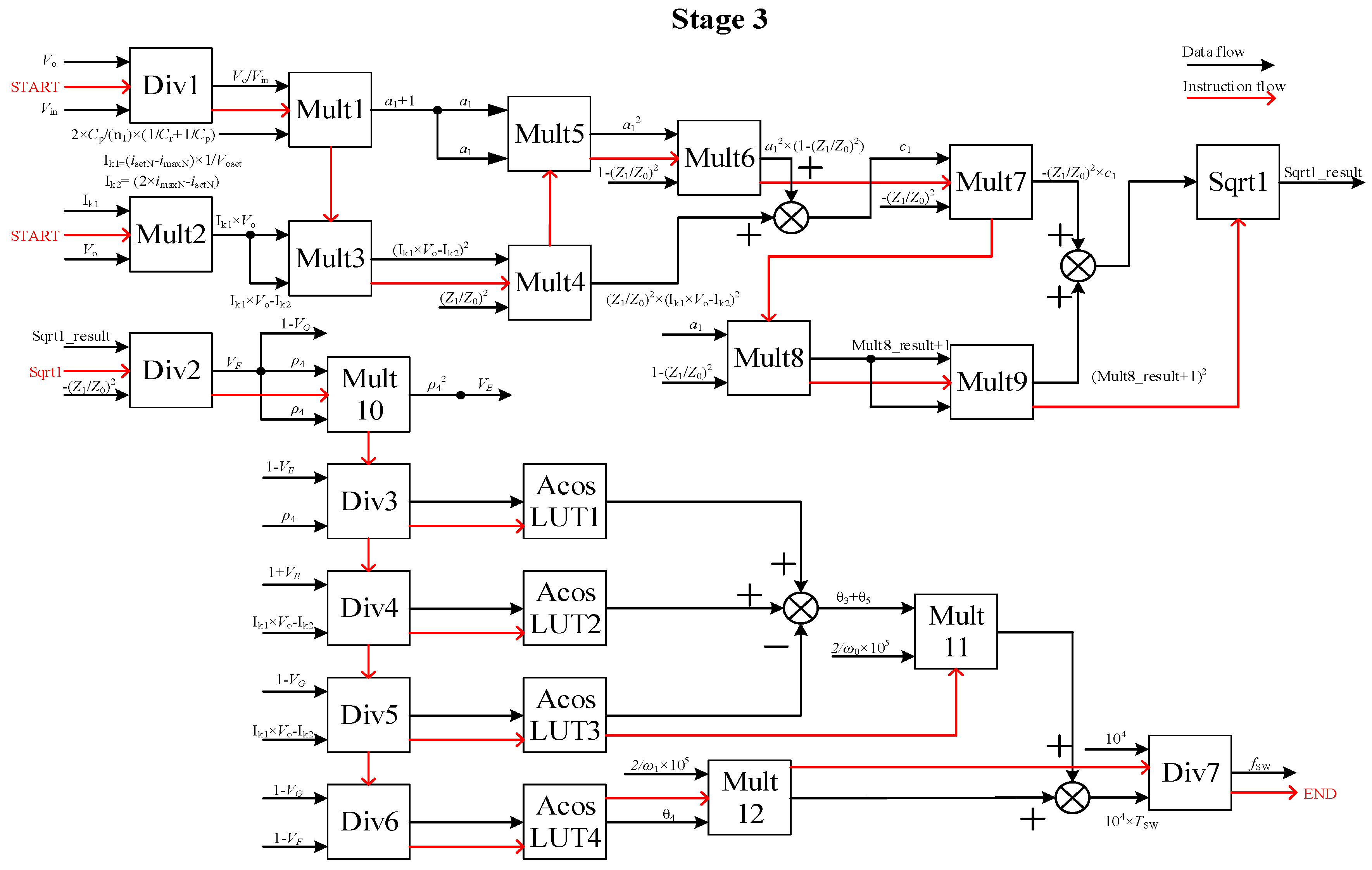
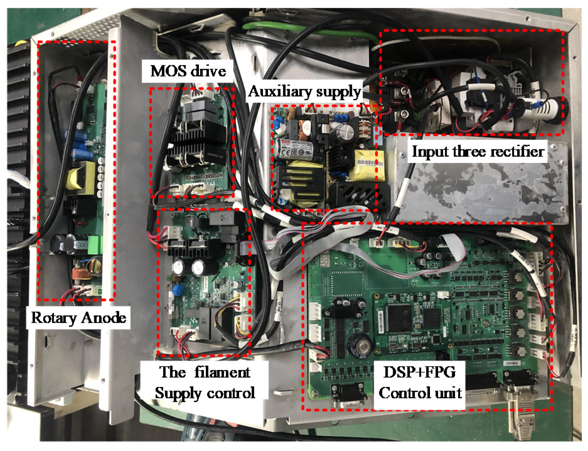
3. Implementation of State Trajectory Control Based on FPGA

In stage 1, T0 and T1 are calculated by DSP, and then the data of T0 and T1 are sent to FPGA before the LCC converter starts. As shown in Figure 7, all equations in stage 2 are divided into 12 multiplications, 7 division calculations, 2 square root calculations, and 4 inverse trigonometric function calculations. Similarly, in stage 3, the equations are divided into 12 multiplications, 7 division calculations, 1 square root calculation, and 4 inverse trigonometric function calculations.

Figure 7. FPGA Block diagram of stage 2.

In FPGA, division and square root operation modules consume many logic resources. The logic resources of FPGA are seriously wasted when the state trajectory control program is parallel computing. Therefore, the state trajectory control program adopts serial calculation. FPGA has only one division, square root, and inverse trigonometric function module. The red arrow shows the operation sequence of the program.

Figure 7 shows the calculation process of stage 2 in FPGA. As shown in Figure 7, A₁, B_1, and C₁ can be calculated in the 1st, 2nd, and 3rd calculation of multiplication correspondingly. θ₀ can be calculated in the calculation of arcsine. θ₁ can be calculated in the 3rd calculation of arc cosine. θ₂ is the difference between the 2nd and 1st calculation of arc cosine.

Figure 8 shows the calculation process of stage 3 in FPGA. As shown in Figure 8, a₁ can be calculated in the 1st calculation of multiplication, and c₁ is the sum of the 4th and 6th calculations. θ₃ + θ₅ can be calculated when the 3rd calculation of arc cosine is completed. θ₄ can be calculated in the 4th calculation of arc cosine.

Figure 8. FPGA Block diagram of stage 3.

The data in FPGA is stored in 25-bit fixed-point register. The 25th bit of the register is used to store the sign of data. The 17th to 24th bits are used to store integer data. The 1st to 16th bits of the register are used to store decimal data. FPGA can not directly process decimal, so the CORDIC(Coordinate Rotation Digital Computer) algorithm is used in the division and square root operation module. The look-up table is used to operate the inverse trigonometric function.

The calculation speed of the state trajectory control in FPGA is significantly faster than that in DSP. The calculation time of state trajectory control in DSP28335 needs more than 20 us. But it just takes 200 clock cycles to complete all calculations of state trajectory control in FPGA, and the calculation time is less than 2us. In FPGA, each division and square root operation requires 17 clock cycles, and Multiplication and inverse trigonometric function operations require 4 clock cycles.

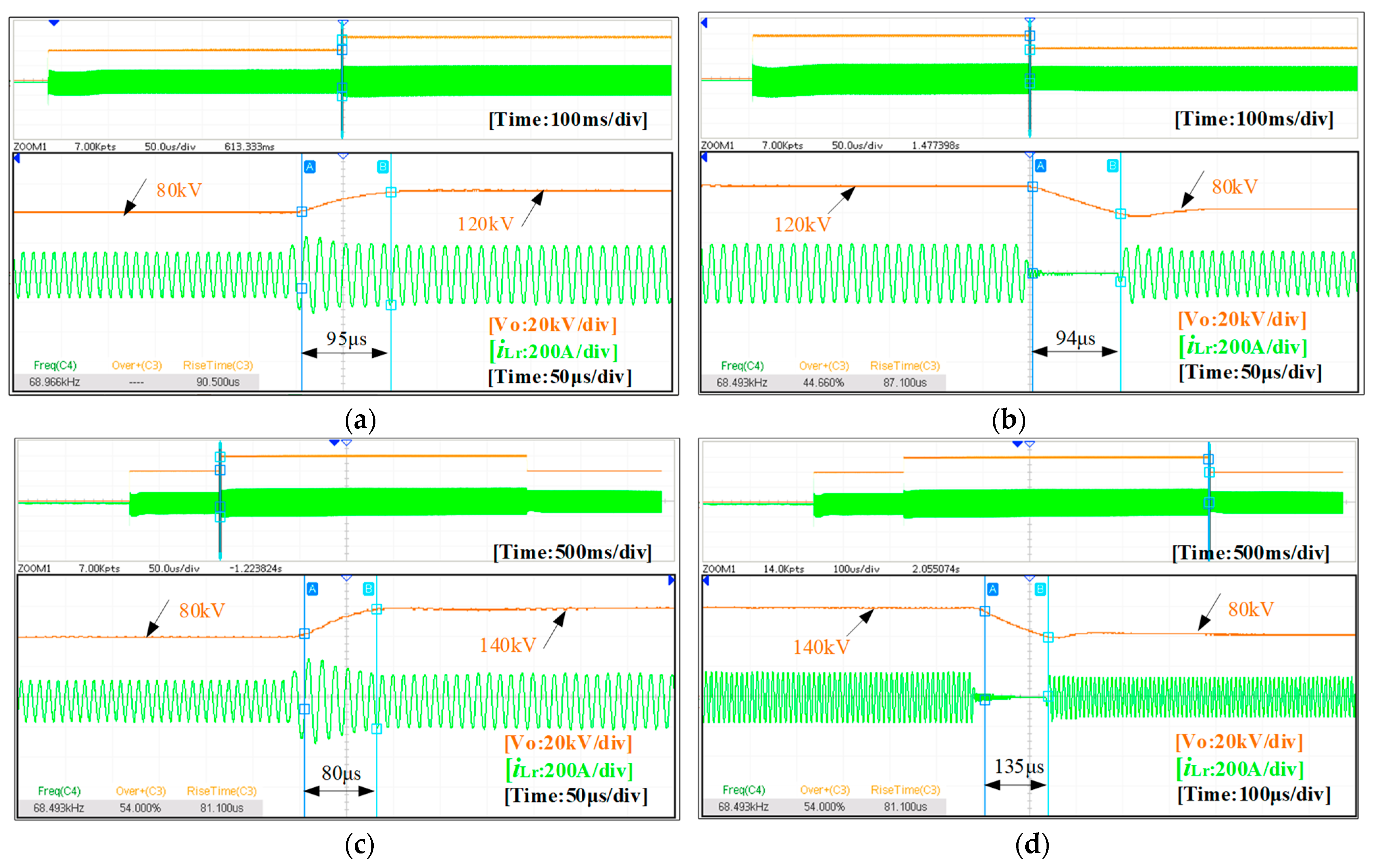
4. Experiment Results

In order to verify the correctness of the proposed control algorithm, the 140 kV/42 kW for the X-ray generator prototype platform was built up, as shown in Figure 9. The experiment parameters are listed in Table 2.

Figure 9. Prototype of the 140kV/42kW.

Table 2. The circuit paraments of prototype.

Parameters	Value
Output Power (P)	42 kW
Input voltage (Vin)	500 ± 50 V
Output voltage (Vo)	60 kV~140 kV
Output current (Io)	10 mA~350 mA
Load (RL)	512 kΩ
Transformer Ratio	15:301 (6)
Resonant inductor (Lr)	30 μH
Series Resonant capacitor (Cr)	0.66 μF
Parallel Resonant capacitor (Cp)	0.266 μF
Switching frequency (fsw)	70~120 kHz

As shown in Figure 10a, the exposure time of the X-ray generator is set to 10 ms. And the output voltage V_o is 100 kV, i_max is set as 200 A, the resonant tank current achieves the set value of 200 A during the first cycle, and no extra voltage or current overshoot is injected into the resonant circuit. A fast rise time is achieved during the startup process, where (10–90%) of V_o is 350 μs. At the same time, for conventional PFM control, the experiment waveforms at startup are presented in Figure 10b A fast rise time is achieved during the startup process. Based on the same circuit parameters and classical PI control, the rise time of the output voltage of the generator is 1.182 ms.

Figure 10. Experimental waveforms: (a) Waveforms of startup with OTC; (b) Waveforms of startup with conventional PFM.

Figure 11a–d shows the experimental waveforms of output voltages under closed-loop control to further verify the proposed control scheme for the transient state. The switching process of different kV levels is presented between 140 kV, 120 kV, and 80 kV to achieve a faster transient time and keep the resonant tank’s voltage or current from overshoot. The control strategy combines the benefits of OTC and PI. It has an excellent dynamic characteristic with a rise time of less than 100μs and a fall time of less than 150 μs under the resistive load, which benefits from the resonant tank being precisely controlled. Therefore, the validity of the proposed OTC is verified.

Figure 11. Experimental waveforms of switching process of different kV: (a) From 80 kV to 120 kV; (b) From 120 kV to 80 kV; (c) From 80 kV to 140 kV; (d) From 140 kV to 80 kV.

5. Conclusions

In this paper, a novel topology of ISOS Type LCC-SPRC is presented. The starting strategy of the LCC converter based on state trajectory control is analyzed in detail, and a state trajectory control based on FPGA for LCC resonant converter is proposed. Finally, the proposed approach has been implemented in FPGA and DSP. The experimental results on a 140 kV/42 kW X-ray imaging system generator show the model’s good dynamics and the control scheme’s implementation ability and significantly reduce the rising time of output voltage.

References

1. Moskalev, Y.A.; Buller, A.I.; Babikov, S.A. Luminescent convertors of X-ray radiation for medical and engineering diagnostics and systems for nondestructive testing. Russ. J. Nondestruct. Test. 2011, 41, 730–734. [Google Scholar] [CrossRef]
2. Villegas, P.J.; Díaz, J.; Pernía, A.M.; Martínez, J.A.; Nuño, F.; Prieto, M.J. Filament Power Supply for Electron Beam Welding Machine. IEEE Trans. Ind. Electron. 2015, 62, 1421–1429. [Google Scholar] [CrossRef]
3. Bae, J.; Jang, S.; Kim, H. Design of Ion Pump Power Supply Based on LCC resonant converter. IEEE Trans. Power. Electron. 2018, 46, 3504–3511. [Google Scholar]
4. Soeiro, T.B.; Muhlethaler, J.; Linner, J.; Ranstad, P.; Kolar, J.W. Automated design of a high-power high-frequency LCC resonant converter for electrostatic precipitators. IEEE Trans. Ind. Electron. 2013, 60, 4805–4819. [Google Scholar] [CrossRef]
5. Mao, S.; Li, C.; Li, W.; Popovic, J.; Schroder, S.; Ferreira, J.A. Unified equivalent steady-state circuit model and comprehensive design of the LCC resonant converter for HV generation architectures. IEEE Trans. Power. Electron. 2018, 33, 7531–7544. [Google Scholar] [CrossRef]
6. Fan, S.; Li, H.; Wang, Z.; Yuan, Y. Time domain analysis and efficiency research of high voltage power supply for electron beam welder based on LCC resonance in DCM. In Proceedings of the 2017 20th International Conference on Electrical Machines and Systems (ICEMS), Sydney, Australia, 11–14 August 2017; pp. 1–5. [Google Scholar]
7. Jafari, H.; Habibi, M. High-voltage charging power supply based on an LCC-type resonant converter operating at continuous conduction mode. IEEE Trans. Power Electron. 2020, 35, 5461–5478. [Google Scholar] [CrossRef]
8. Feng, W.; Lee, F.C.; Mattavelli, P. Simplified optimal trajectory control (SOTC) for LLC resonant converters. IEEE Trans. Power Electron. 2013, 28, 2415–2426. [Google Scholar] [CrossRef]
9. Feng, W.; Lee, F.C. Optimal trajectory control of LLC resonant converters for soft startup. IEEE Trans. Power Electron. 2014, 29, 1461–1468. [Google Scholar] [CrossRef]
10. Feng, W.; Lee, F.C.; Mattavelli, P. Optimal trajectory control of burst mode for LLC resonant converter. IEEE Trans. Power Electron. 2013, 28, 457–466. [Google Scholar] [CrossRef]
11. Fei, C.; Lee, F.C.; Li, Q. Digital Implementation of Light-Load Efficiency Improvement for High-Frequency LLC converters with Simplified Optimal Trajectory Control. IEEE Trans. Power Electron. 2018, 6, 1850–1860. [Google Scholar] [CrossRef]
12. Fei, C.; Lee, F.C.; Li, Q. Digital implementation of soft startup and short-circuit protection for high-frequency LLC converters with optimal trajectory control (OTC). IEEE Trans. Power Electron. 2017, 32, 8008–8017. [Google Scholar] [CrossRef]
13. Zhao, J.; Wu, L.; Chen, G. State Trajectory Control of Burst Mode for LCC Resonant Converters with Capacitive Output Filter. IEEE Trans. Power Electron. 2022, 37, 377–391. [Google Scholar] [CrossRef]
14. Jang, S.-R.; Seo, J.-H.; Ryoo, H.-J. Development of 50-kV 100-kWthree-phase resonant converter for 95-GHz gyrotron. IEEE Trans. Ind. Electron. 2016, 63, 6674–6683. [Google Scholar] [CrossRef]
15. Fei, C.; Li, Q.; Lee, F.C. Digital implementation of adaptive synchronous rectifier (SR) driving scheme for high-frequency LLC converters with microcontroller. IEEE Trans. Power Electron. 2018, 33, 5351–5361. [Google Scholar] [CrossRef]
16. Martin-Ramos, J.A.; Diaz, J.; Nuno, F.; Villegas, P.J.; Lopez-Hernandez, A.; Gutierrez-Delgado, J.F. A polynomial model to calculate steady-state set point in the PRC-LCC topology with a capacitor as output filter. IEEE Trans. Ind. Appl. 2015, 51, 2520–2527. [Google Scholar] [CrossRef]
17. Ahn, S.-H.; Jang, S.-R.; Ryoo, H.-J. High-efficiency bidirectional three-phase LCC resonant converter with a wide load range. IEEE Trans. Power Electron. 2019, 34, 97–105. [Google Scholar] [CrossRef]
18. Chen, Y.; Xu, J.; Gao, Y.; Lin, L.; Cao, J.; Ma, H. Analysis and design of phase-shift pulse-frequency-modulated full-bridge LCC resonant converter. IEEE Trans. Ind. Electron. 2020, 67, 1092–1102. [Google Scholar] [CrossRef]
19. Shi, W.; Deng, J.; Wang, Z.; Cheng, X. The startup dynamic analysis and one cycle control-PD control combined strategy for primary side controlled wireless power transfer system. IEEE Access 2018, 6, 14439–14450. [Google Scholar] [CrossRef]
20. Zhang, S.; Li, L.; Zhao, Z.; Fang, S.; Wang, C. Optimal trajectory based startup control of LCC resonant converter for X-ray generator applications. In Proceedings of the 2nd International Conference on Power Engineering (ICPE 2021), Nanning, China, 9–11 December 2021. [Google Scholar]
Publisher’s Note: MDPI stays neutral with regard to jurisdictional claims in published maps and institutional affiliations.
Article Metrics
Citations
Article Access Statistics
Multiple requests from the same IP address are counted as one view.