Abstract
Lane detection is an essential module for the safe navigation of autonomous vehicles (AVs). Estimating the vehicle’s position and trajectory on the road is critical; however, several environmental variables can affect this task. State-of-the-art lane detection methods utilize convolutional neural networks (CNNs) as feature extractors to obtain relevant features through training using multiple kernel layers. It makes them vulnerable to any statistical change in the input data or noise affecting the spatial characteristics. In this paper, we compare six different CNN architectures to analyze the effect of various adverse conditions, including harsh weather, illumination variations, and shadows/occlusions, on lane detection. Among all the aforementioned adverse conditions, harsh weather in general and snowy night conditions particularly affect the performance by a large margin. The average detection accuracy of the networks decreased by 75.2%, and the root mean square error (RMSE) increased by 301.1%. Overall, the results show a noticeable drop in the networks’ accuracy for all adverse conditions because the features’ stochastic distributions change for each state.
1. Introduction
Recent progress in electric vehicles, telecommunications, machine learning, tracking technologies, and robotics have opened opportunities for deploying autonomous vehicles (AVs) on urban roads and highways.
Current green automotive policies seek to reduce greenhouse gas emissions to zero. This has led to electric vehicles becoming the standard platform for AV development [1,2]. Many countries, such as Canada and the United States, have aimed for electric, hybrid, or hydrogen-powered vehicles to dominate the market by 2035 [3].
Unfortunately, AVs face particular problems, including high energy consumption, navigation system performance, and road safety. Any inadequate motion execution on the road may lead to an accident and increase energy consumption.
The different sensors needed, such as light detection and ranging (LiDAR) or radar, and the processing of the different data, are responsible for the high energy consumption of AVs. This reduces the autonomy of the vehicles considerably. One proposed solution is to use a single type of sensor, namely a camera [4].
Regarding the navigation system, any unknown element on the road will make it challenging to recognize the driving area, causing the system to fail. This is because it relies heavily on visual perception to interpret the surrounding environment.
Although lane departure warning/prevention (LDW/LDP) systems can prevent 297,000 lane departure accidents annually, the accident rate due to this is still very high. In 2015, the United States recorded 13,000 fatalities due to unintentional lane departure [5].
For any autonomous navigation module, two challenges must be tackled: (i) the perception of the environment, specifically the road markers and signs, and (ii) the planning and execution of an appropriate motion for driving the vehicle safely to a given destination.
Different external variables cause visual conditions to be less than ideal, thus affecting the perception of road markings and signs. Variables such as weather (snow, fog, rain), time of day, and lighting changes increase the detection complexity [6,7].
In the meteorological context of countries where winter involves snow, people and AVs have difficulty perceiving and recognizing road markings and signs due to snowfall and ice accumulation. Drivers must rely on their intuition and memory of the road to maintain proper lanes because they cannot differentiate road markings whose color is diminished by snow [8]. AVs do not have specific skills for driving in snow. They use camera-based techniques, so their performance decreases significantly when the lane is not easily visible.
Researchers should strive to optimize AVs’ systems, such as navigation and driver assistance, and ensure they function correctly without affecting the vehicle’s autonomy.
This paper provides an experimental analysis of the effects of several challenging environmental driving conditions on the performance of regression-based neural networks applied to lane recognition. A benchmark of six commonly used architectures (alexNet, resNet-18, resNet-50, squeezeNet, VGG16, and NASNet) is performed, using their performances under normal environmental conditions as a reference.
We have observed how much the accuracy rate of these algorithms in predicting lane lines decreases as the conditions of the road scenario vary. These challenging conditions include snow, different times of day, and shaded areas.
The contributions of our paper can be summarized as follows:
- In many lane recognition studies, it is assumed that deep learning algorithms can perform well in scenarios with some degree of similarity to the training scenario. Experimentally, this work is intended to verify and demonstrate that the performance of these algorithms is limited. The networks are mainly based on feature extraction from the inputs and statistical dependencies, so they will not adapt well if there are changes or noise in these data.
- As it is unknown to what extent snow accumulation on the road makes lane prediction difficult, we wanted to delve deeper into this scenario. Three scenarios with different amounts of snow on the lane, in both day and night, are included among the test conditions. Future work may use the limitations encountered to develop an approach to combat them.
The rest of the paper is arranged as follows. Section 2 reviews the background of lane detection methods. Section 3 presents our experiment with six deep learning algorithms. The study’s results are displayed in Section 4, and the discussion is in Section 5. Section 6 consists of the conclusions and future work.
2. Related Work
The lane detection system is one of the AVs’ perception modules, essential to ensure safe navigation. In recent years, different methods have been proposed and developed for lane detection and prediction [9]. We can find different surveys of vision-based lane recognition systems and advances in this area and LDW systems.
Narote et al. [10] addressed the different modules of the vision-based lane recognition systems in their survey, such as video capture, lane modeling, feature extraction, and lane tracking. Tang et al. [7] also included optimization strategies for these methods, which aimed to obtain good performance with a smaller dataset or to avoid post-processing. Ghani et al. [11] reviewed different lane detection algorithms, considering weather conditions such as fog, haze, or rain. Additionally, they proposed a new contour angle method for lane marker classification. Xing et al. [12] focused on and analyzed systems in detail, which included information on methodologies that integrate such lane recognition algorithms with sensors or other systems. They analyzed a lane detection framework based on the ACP (artificial society, computational experiments, and parallel execution) theory, which consists of constructing parallel virtual scenarios for model training. They highlighted that it is a possible way to solve generalization problems.
Specifically to recognize the driving zone, researchers use both traditional and deep learning-based methods. Among the former is geometric modeling of traffic lines [7,13], which uses information such as color, texture, edges, and gradient. Energy minimization modeling has also been used.
Jung and Bae [14] presented a prototype for real-time road lane detection using data acquired through a 3D LiDAR sensor and for the automatic generation of lane-level maps. The authors initially distinguished traffic signal points on the ground from LiDAR data. They used an expectation-maximization method to detect parallel lines and update the 3D line parameters as a vehicle moved forward. Finally, they built a lane-level digital map from these parameters and a GPS (global positioning system)/ins (inertial navigation system) sensor.
Many deep learning-based algorithms have been used in the field of lane detection. These include the early CNN-based method, encoder–decoder CNNs [15,16], fully convolutional neural networks (FCNs), or combinations of CNNs and recurrent neural networks (RNNs) [9,17]. Likewise, generative adversarial networks (GANs) have been shown to be suitable for expressing complex line shapes [7,18].
According to Tang et al. [7], the lane detection task can be approached from three perspectives. The first approach is classification-based methods, which use prior information to obtain the lane position or discriminate the road boundary type [19,20]. The second approach consists of object detection-based methods where feature points for each lane segment and coordinate regression are used [21,22]. The third perspective encompasses segmentation-based methods [15,18,23,24,25], which classify the pixels of an input image into individual classes. All of these use feature extractors via learning.
With the victory of the AlexNet network in the ImageNet Large-Scale Visual Recognition Challenge (ILSVRC) in 2012, deep learning, especially CNNs, have gained significant momentum. This has become a promising tool in several application fields, including lane marking detection [7], where they have effectively improved the accuracy and robustness of this task [26].
Neven et al. [15] proposed the LaneNet fast lane detection algorithm, which can identify a variable number of lanes, thus allowing to deal with lane changing. The authors employed an instance segmentation method that can be trained end-to-end, where each lane forms its instance. They also proposed using a learned perspective transformation to the parameterize of the segmented lane instances, thus obtaining a solid lane adjustment against road plane changes.
Some strategies have been addressed to optimize deep learning methods by avoiding post-processing or obtaining good performance using fewer data. One of these strategies is using pre-trained models and configuring and adapting them according to the problem of interest. There are two approaches: transfer learning and knowledge distillation methods [7,27]. These take advantage of the pre-trained layers of the original model, using the first layers to recognize the most generic features [28]. Subsequent layers are kept or removed or new ones are added depending on the problem to be addressed and the expected results [27].
In the study of Kim and Park [16], they presented a sequential transfer learning method for the ego-lane estimation that considers all the information of an input image during training. This method consists of the SegNet network, an end-to-end deep encoder–decoder architecture built on region segmentation. The authors reported direction estimation accuracies with augmented test data between 66% and 69% for a single transfer learning network and direction accuracies between 76% and 81% for a sequential transfer learning network. In [29], Zhang et al. developed an adaptive learning algorithm for lane features using KITTI and Caltech datasets. They built a two-stage learning network based on the YOLO v3 (You Only Look Once, v3) algorithm, whose parameters were modified to suit lane detection. For the KITTI dataset, the authors reported accuracies of 79.26%, and for the Caltech dataset, 81.75%. Other lane detection algorithms such as Fast RCNN or sliding window & CNN evidenced accuracies of 49.87% and 68.98%, respectively, for the KITTI dataset. Hou et al. [30] used the self-attention distillation (SAD) method, which they incorporated into a CNN for lane detection. This method consists of a model learning from itself by continuously improving without additional labels or supervision. The authors validated the method using three road lane databases: TuSimple, CULane, and BDD100K. They use ENet, ResNet-18, and ResNet-34 architectures, obtaining accuracies of 92.69%, 92.84%, and 93.02%, respectively. Hou et al. found that the performance of the ENet–SAD model was good, with an accuracy of 96.64%, surpassing the existing algorithms, while being faster and requiring fewer parameters. Transfer learning has shown great promise as it helps decrease training time, reduce computations, and make training more efficient [27,28].
Table 1 presents a summary of some CNN-based lane detection methods based on the network, the dataset used, and the metrics selected for evaluating the methods.

Table 1.
Summary of some CNN-based lane detection methods.
Concerning other deep learning models, the RNN networks, composed of loops, are used to analyze time series data, e.g., for speech recognition, language recognition, or handwriting. These present the problem of long-term dependency, where they cannot remember information for long periods. However, a type of these networks can deal with this problem, the long short-term memory (LSTM) [35] network. In the literature, we can find studies that have used these networks for lane detection; however, they are combined with others techniques, such as CNNs, which are used as feature extractors.
Zou et al. [9] developed a deep hybrid architecture for lane recognition. This combines a CNN for abstracting information from each frame of a driving scene, and an RNN, for lane line prediction based on the features extracted by the CNN. This method proved to be adequate, outperforming other methods used for lane detection, even in difficult situations. Kortli et al. [36] proposed a real-time lane detection system based on a CNN encoder–decoder network and an LSTM network. The encoder extracts the features and reduces the dimensionality, the decoder maps those features, and the LSTM network processes the data to improve the detection rate. The study showed a good performance with 96.36% accuracy. Wu et al. [37] presented an approach that uses a gradient map to emphasize lane features such as edges or color differences instead of using RGB images as inputs. This approach was used to train a CNN network based on VGG-16, observing an increase in accuracy and a reduction in training and inference time as compared to networks trained with RGB images. Similarly, an LSTM network was trained with the gradient map as an input to improve the detection of obscured lanes due to occlusions or varying lighting conditions. The above showed better performance than the CNN network alone.
Transformers are architectures that adopt the attention mechanism, focusing on specific parts of an input based on the importance [38]. They accept sequential input data but do not always process them in order, reducing training time due to parallelization. These models are often used in language and image processing, where they have obtained similar results to CNNs [39].
There is not yet much research in lane detection that rely on transformers; however, the study of Liu et al. [40] stands out. They use transformers to predict the polynomial parameters of a lane shape model using a self-attenuation mechanism to focus on the long and thin structures of the lanes and the global context. This research yielded good accuracy results when testing the model on the TuSimple dataset (96.18%), while being fast and light in size. It also demonstrated good adaptability to scenarios with nighttime conditions or with occluded parts; however, it does not address complex lane detection tasks. Likewise, in [41], Han et al. developed the Laneformer transformer-based architecture and adapted it to lane detection. This better captures the lane shape characteristics and the global semantic context of the series of points defining the lanes using a row and column self-attenuation mechanism. Unlike [40], this model predicts the points in each lane to adapt to more complex scenarios. The architecture included a ResNet-50 backbone to extract basic features. This was evaluated on the CULane and TuSimple datasets, performing well in both normal environmental conditions and night or glare scenarios.
Among other lane detection methods is the algorithm proposed by Cao et al. [26]. This study covers road environments with poor illumination, winding roads, and background interference, including highway, mountain, and tunnel roads. Using the random sample consensus algorithm, the authors obtained an aerial view of the road and fit the lane line curves based on the third-order B-spline curve model. The method obtained a 98.42% detection accuracy.
Despite the research, there is still little work on lane recognition on winter roads, both day and night, and little research evaluating the performance of neural networks applied to such situations. Some works cover different lighting conditions, and others focus on fog or rain; however, the conditions covered in this work have not been addressed to a large extent.
3. Benchmarking Design
The benchmarking was developed to analyze the impact of different environmental driving conditions on the performance of the most widely used backbones CNNs in deep learning-based lane detection methods. Quantitative and qualitative analysis is performed to review this impact comprehensively.
This section describes the design of the different training and testing experiments performed. The selected dataset and the challenging driving environment conditions are covered in the first instance. We continue with selecting the evaluated networks and their training parameters and end with the study’s metrics.
3.1. Dataset
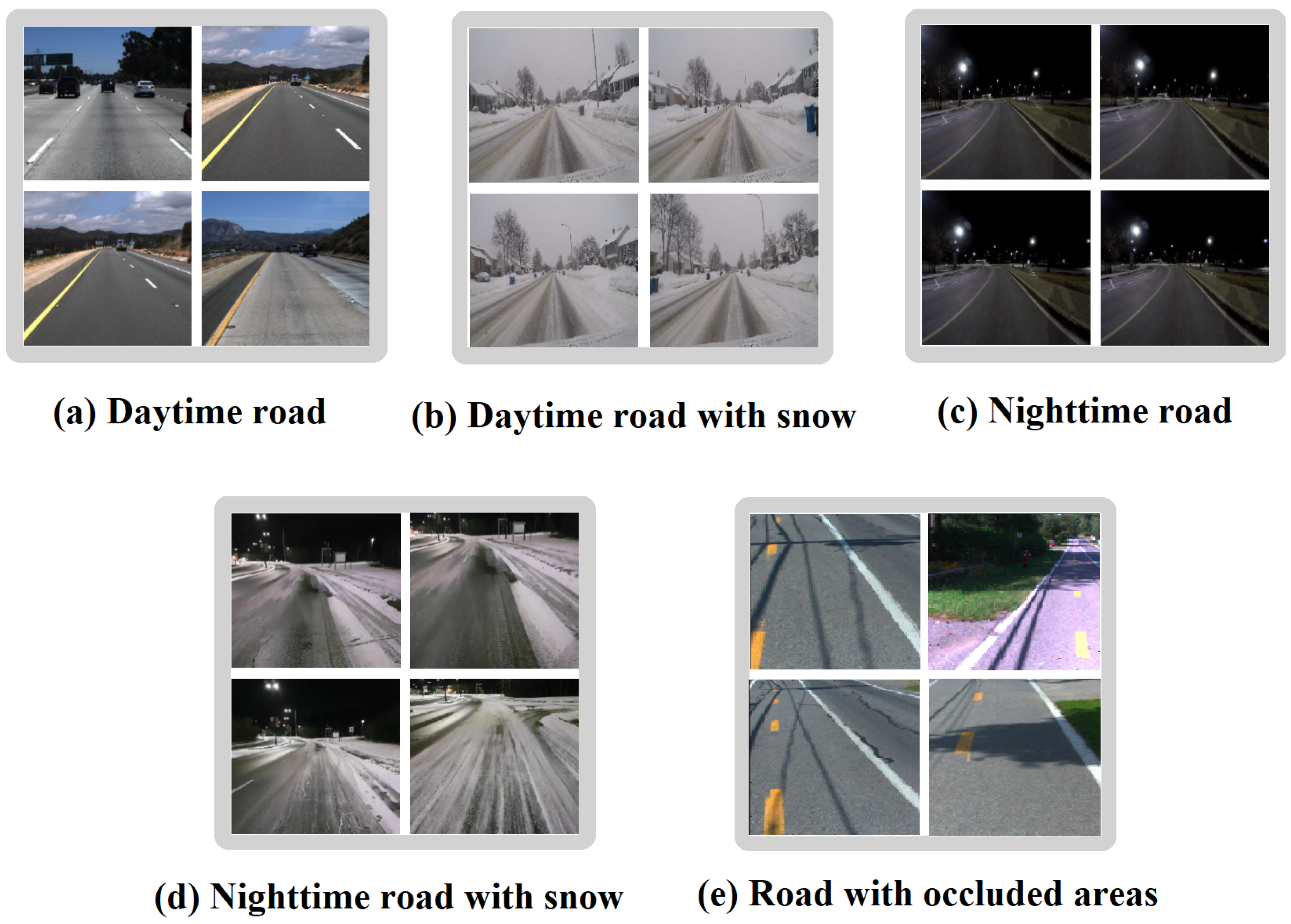
Two road datasets have been used for this study. The first one is the TuSimple dataset [42] which includes mild weather conditions and was used to train the networks. The second is a locally captured dataset consisting of images with challenging weather conditions, such as snow or night road. This dataset was used to test the performance of the previously trained architectures. Figure 1 shows the datasets used in this study with the different environmental situations of interest.

Figure 1.
Environmental driving conditions datasets. TuSimple dataset: (a) Daytime road under normal conditions. Our own dataset: (b) Daytime road with snow, (c) nighttime road under normal conditions, (d) nighttime road with snow and (e) road with occluded areas. Source: [42].
3.1.1. Good Weather Conditions Dataset
We used the open-access TuSimple dataset [42] for training the networks. This has a set of video clips with a total of 6408 images of U.S. roads with resolutions of 1280 × 720. The database includes good and average weather conditions, different traffic conditions, and roads with two or more lanes. The images corresponding to the last frame of each clip have annotated lane marking (current lane, left, and right) indicating the position through x and y values concerning the point of origin of the image.
For this study, it was decided to use a set of 3500 images from the selected dataset, dividing it into 70% training data and 30% test data.
3.1.2. Challenging Environmental Conditions Dataset
A locally captured dataset was included to evaluate the performance of the trained networks against harsh environmental conditions. The setup consisted of a GoPro HERO5 Black camera mounted on the hood of the Kia Soul EV from the Université du Québec à Trois-Rivières. The dimensions of the images captured with this system are 1920 × 1080 pixels.
3.1.3. Image Preprocessing
The selected images were adjusted to the network architectures’ input layer size. This change was made to avoid the high computational cost and reduce the training time involved in processing images with huge resolutions [32]. Similarly, by reducing the images’ size, the networks can see key features in the initial layers, which would otherwise be learned at the network’s end [43]. The input image resolutions were set at 227 by 227, 224 by 224, and 331 by 331, depending on the network.
The approaches generally used to resize input images to neural networks are border pixel cropping, and downsampling using interpolation. However, the former implies losing features or patterns in border areas, and the latter implies deformations of parts or patterns in the image [44]. For our study, we consider two points before determining which image resizing approach to choose.
The data used in our study have an original size of 1920 × 1080 for the challenging environmental conditions dataset and 1280 × 720 for the TuSimple dataset. This size is significant in relation to the size of the input layer of the evaluated networks. If we consider cropping the original picture, the resulting image will be insufficient, as it will only include a small part of the street. Regions with important road and environmental features necessary for the network to predict lane locations will be lost.
We considered methods based on object detection by labeling regression feature points for each lane segment, so it is essential to have a global view of the road. By resizing the images by downsampling, they could be deformed by changing the aspect ratios. Despite this, the images still have a complete picture of the road so that the network can predict the position and curvature of the lane boundaries. Additionally, by having a view of the environment, the networks may be able to use other static features, such as buildings, to delimit the lane. By resizing the picture by cropping, one does not have an overall view of the road. The resized image would only show a small segment of the lane, and its coordinates with respect to the road could not be predicted. This small segment could even be occluded in challenging environmental conditions, with the network not having sufficient features to extract.
Considering the images’ original size and our study’s encompassing a regression problem where the network predicts the lane coordinates, we resized the images by downsampling using a bicubic interpolation method. This is because it is less risky to deform image features than to lose them [44]. Likewise, by resizing the images by downsampling, it was observed that the pictures do not lose the details needed to delimit the road lane.
We labeled the images using the Ground Truth Labeler app [45] from the MATLAB Automated Driving System Toolbox™ [46] along with the “Lane Boundary Detector” algorithm. In the images, the ego-lane was defined by polylines formed by seven points each. Considering that not all coordinates in X for the labels were at the same height, to facilitate training we decided to recalculate these values for fixed Y values by calculating the lane line coefficients of a second-order polynomial. Figure 2 shows a diagram describing the labeling procedure underwent [47].

Figure 2.
Labeling procedure description. Source: [42,45].
As an essential part, we had to convert the dataset into a 4D matrix to process the images in the networks using MATLAB correctly.
3.2. Challenging Driving Environment Conditions
Some factors related to the driving environment may affect lane detection performance and even more so if algorithms are designed and tested for a specific situation. It is necessary to know and evaluate such variation in performance, as well as the more significant number of influencing factors, to improve the inclusion and robustness of the lane recognition algorithm as well as the stability and reliability of detection under various conditions [12,26].
We address four particularly challenging environmental situations for AVs and humans, which are listed below. The networks were tested on 100 images in each situation, and lane prediction was evaluated against ground truth labels. This was to explore as to what extent the performance of the evaluated networks differed from their performance on daytime roads under normal environmental conditions.
- Nighttime road under normal conditions.
- Daytime road with snow. We explore two situations: daytime road with light snow and daytime road with moderate snow.
- Nighttime road with snow.
- Road with occluded areas.
3.3. Pre-Trained Networks
The deep learning-based methods were chosen based on the work’s objectives of evaluating their performance in similar scenarios to the training scenario but different in terms of climate and illumination. Thus, we took pre-existing and pre-trained networks and adapted and fine-tuned them to detect lane boundaries.
We decided to evaluate CNNs, considering that all learning-based methods somehow use feature extractors. Another reason for this choice is the high detection accuracy of this type of networks [48]. That makes CNNs among the most famous and employed algorithms in computer vision, including for identifying lane boundaries [20,49]. In particular, we considered methods based on object detection by labeling regression feature points for each lane segment.
Currently, there are several pre-existing networks such as AlexNet, GoogLeNet, VGG, ResNet, Inception, and MobileNet, among others [50]. Most of these architectures were pre-trained using the ImageNet database [51] used at ILSVRC [52]. According to Canziani et al. [53], different variables can be considered when choosing between these networks. These variables include accuracy, memory footprint, parameters, operation count, inference time, and power consumption. Based on this, the following networks were selected for this study: AlexNet, SqueezeNet, ResNet-18, ResNet-50, VGG16, and NASNet. These are described below.
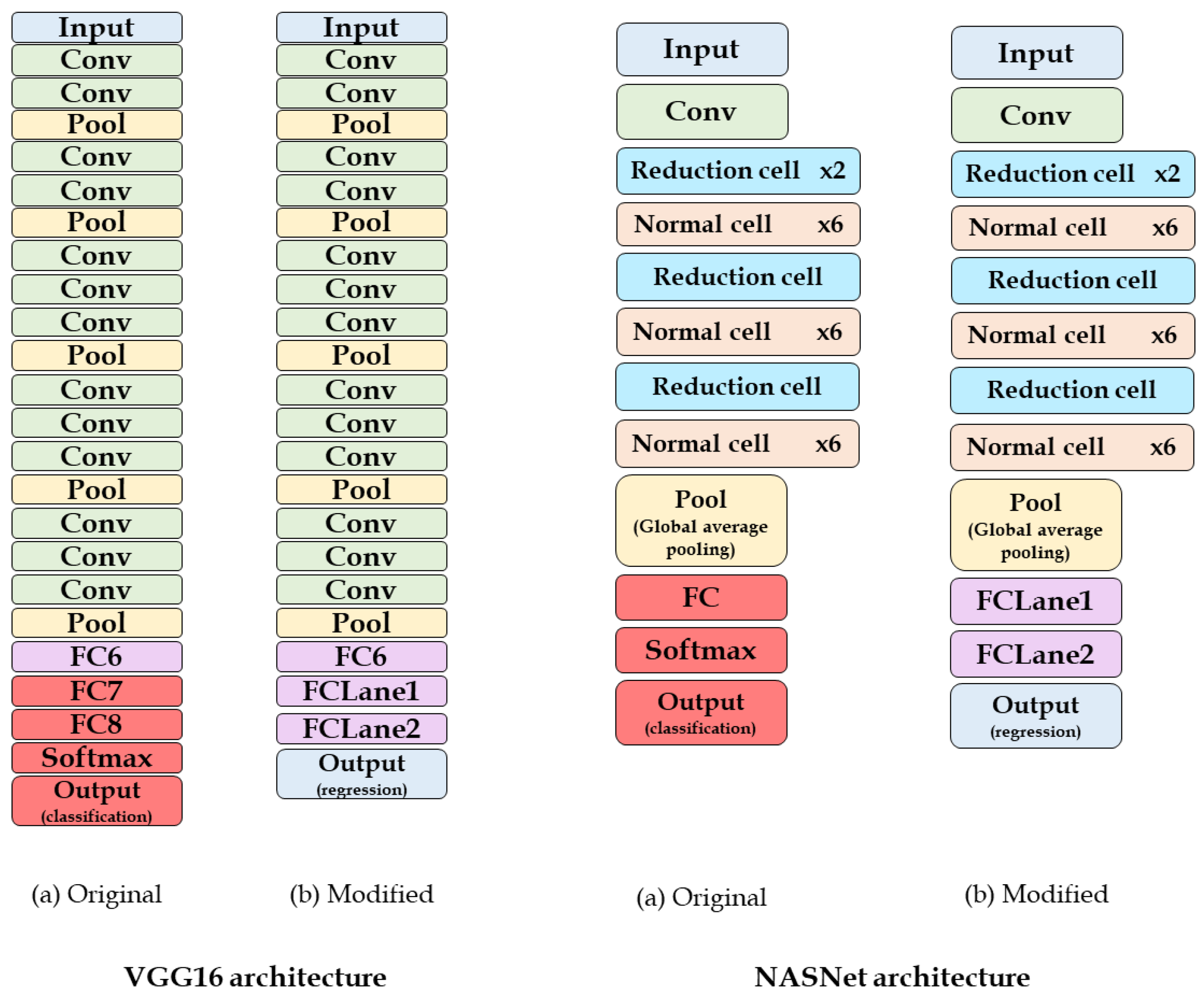
In general, for the fine-tuned networks, we replaced only the last layers of the models, adjusting them to our data, and kept the previous layers unchanged. The final two fully connected layers, or one as the case may be, were replaced with others of appropriate size according to the outputs for each training image. The last of these was assigned 28 responses based on the x and y coordinates of the seven points on each lane line per image. We substituted the final rectified linear unit (ReLU) with a new ReLU as a non-linear activation function [54]. We removed the last dropout layer to avoid poor inference time performance [55]. According to Rasmussen [55] and Allohvk [56], the dropout layer does not work well for a task whose output represents an absolute quantity, as in our case. It works better with relative values, such as the softmax classification. Finally, we replaced the softmax and the classification layer with a regression layer to predict the coordinates of the road lane line points. To better understand the modifications made to the networks, we include diagrams of both the original and the new structure throughout this subsection. The fine-tuned layers are highlighted in red in the original architecture.
3.3.1. AlexNet
Considering the variables of speed, accuracy, and size of the networks, we initially decided to use AlexNet, a popular CNN. AlexNet is one of the fastest networks and has a reasonable accuracy rate. This allowed us to quickly iterate and test different settings regarding data preprocessing and training parameters [50] to select the most suitable configuration for the experiment.
AlexNet has eight depth layers, five convolutional layers, and three fully connected layers [57]. The network has an image input size of 227 by 227 [58] and is a suitable feature extractor [31]. Because this is a classification network, its structure was modified to convert it into a regression network to predict the coordinates of the road lane line points. The last two fully connected layers were replaced with others of appropriate size according to the outputs for each training image [31], 28 responses. We substituted the last rectified linear unit (ReLU) with a new one, removed the last dropout layer, and replaced the softmax and the classification layer with a regression layer. Figure 3 (left) summarizes (a) the original AlexNet architecture along with (b) the architecture with new additional layers.
3.3.2. SqueezeNet
A network with a smaller size on disk but equivalent accuracy to AlexNet was also assessed. Thus, we selected SqueezeNet, considering its advantages, such as faster training time, lower overhead, and ease of fitting into the computer memory. SqueezeNet is a CNN with eighteen depth layers, which performs similarly to AlexNet but with fewer parameters, fifty times less [59,60]. It was released in 2016 by DeepScale, the University of California, Berkeley, and Stanford University.
We changed the SqueezeNet architecture to make it a regression network, as with AlexNet. Figure 3 (right) summarizes (a) the original SqueezeNet architecture along with (b) the modifications made it. Two fully connected layers and a ReLU layer were added. A regression layer replaced the final two layers. The image input size is 227 by 227 [61].
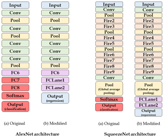
Figure 3.
CNN architectures of AlexNet (left): (a) original, (b) modified; and SqueezeNet (right): (a) original, (b) modified. Source: [62,63,64].
Figure 3.
CNN architectures of AlexNet (left): (a) original, (b) modified; and SqueezeNet (right): (a) original, (b) modified. Source: [62,63,64].

3.3.3. ResNet
We also decided to include a network whose accuracy is superior to that of AlexNet and SqueezeNet in the benchmarking. Considering the computational cost, a low training time was also included in our selection criteria [50]. Thus, the ResNet-18 and ResNet-50 networks, whose accuracy–training time ratio met our requirements, were selected.
ResNet is a residual network proposed by Kaiming et al. [65] in 2015, the year it won the ILSVRC. It was the first to allow training with profound networks by controlling the vanishing gradient problem by omitting one or more layers while presenting good performance [66]. Unlike VGG, ResNet retains its good performance despite removing some layers [67]. Its representation capability has enabled its use in image classification, object detection, and face recognition. There is the ResNet-18 network of eighteen layers deep, the ResNet-50 of fifty layers deep, and ResNet-152 of one hundred and fifty-two layers deep, among others. The deeper the network, the greater the accuracy in more complex tasks.
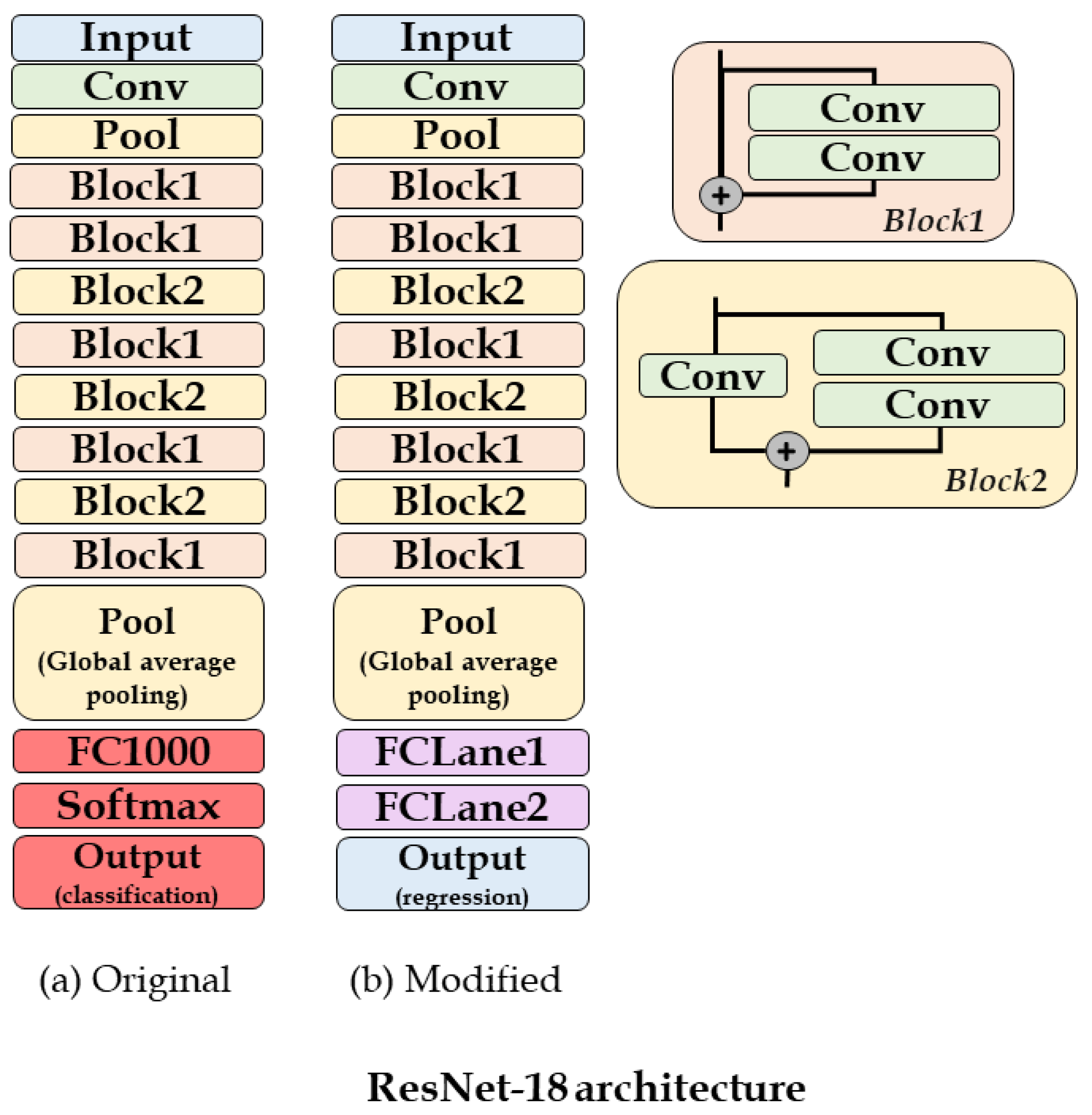
As ResNet-18 and ResNet-50 are classification networks similar to the previous ones, their architecture had to be modified to adapt them to regression networks. In Figure 4, we summarize (a) the original ResNet-18 architecture and (b) the modified architecture. We removed the last fully connected layer and added another fully connected layer with 28 responses according to the coordinates of the seven points of each of the lane lines per image. In the end, the classification layer was changed to a regression layer. The network has an image input size of 224 by 224 [68].
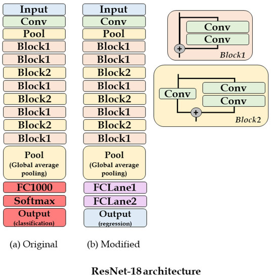
Figure 4.
ResNet-18 architecture: (a) original, (b) modified. Source: [62,69].
3.3.4. VGG16
We also chose to evaluate the VGG network and identify whether and to what extent it outperforms the other architectures. Overall, the performance of VGG is better than the other networks, despite being one of the architectures with higher computational cost and having a more significant number of parameters [7].
There are different VGG network configurations; however, VGG16 has the best performance when tested with the ImageNet dataset. VGG16 is a convolutional neural network with a depth sixteen layers and an image input size of 224 by 224 proposed by Karen Simonyan and Andrew Zisserman [70]. It obtained 92.7% test accuracy on ILSVRC in 2014, becoming one of the most famous architectures [71].
To adapt this network to our problem, we performed the same procedure as the previous ones. The last fully connected layer was replaced with one of an appropriate size and the classification layer was replaced with a regression layer. Figure 5 (left) summarizes (a) the original VGG16 architecture along with (b) the modifications and additions we made.
3.3.5. NASNet
Finally, it was decided to evaluate the neural architecture search network (NASNet) performance in the different environmental scenarios. This is because it has one of the best performance accuracies. NASNet has achieved state-of-the-art results with lower complexity (less FLOPS), fewer parameters, and smaller models than similar networks. This CNN has surpassed DenseNet, Inception, MobileNetV1, and ShuffleNet V1 [72].
NASNet is a machine learning model proposed by Zoph et al. [73] in 2018 using the neural architecture search framework with reinforcement learning [74] and redesigning the search space. It obtained 82.7% top-1 prediction accuracy on ImageNet, being 1.2% better than some of the best architectures [73].
The network has an image input size of 33 by 331 [50]. This consists of normal layers and reductions layers and is not composed of a linear sequence of modules [75,76,77]. We adapt NASNetLarge’s architecture to the lane detection problem by eliminating the last fully connected layer and replacing the classification layers with a regression one. In Figure 5 (right), we summarize (a) the original NASNetLarge architecture and (b) the modified architecture.

Figure 5.
CNN architectures of VGG16 (left): (a) original, (b) modified; and NASNetLarge (right): (a) original, (b) modified. Source: [62,73,78,79].
Figure 5.
CNN architectures of VGG16 (left): (a) original, (b) modified; and NASNetLarge (right): (a) original, (b) modified. Source: [62,73,78,79].
3.4. Training Parameters
The selection of hyperparameters is essential, as they influence a network’s training outcome, giving it a higher or lower response accuracy. We evaluated different possibilities with the MATLAB Experiment Manager application [80] for choosing the hyperparameters. We swept through a range of values defined based on related research (number of epochs, learning rate, batch size, and solver) until we obtained the optimal training options for each network.
ADAM’s optimizer was adopted as a solver to update the network parameters. However, with the stochastic gradient descent with momentum (SGDM) optimizer, the performance of the networks was also good, except for SqueezeNet. Similarly, a learning rate was defined, considering that it should be neither too low nor too high. In the first case, the training would take too much time, while in the second, it may diverge or not have an optimal result [81]. Thus, we selected an initial learning rate of 0.0001. According to Jiang et al. [54], the decay of the learning rate every few epochs during training reduces the magnitude of the parameter updates. Initially, it was decided to test this gradual decrease for our networks’ training, with a learning rate drop factor of 0.8 every 20 epochs, as in the research of Jiang et al. [54]. However, the accuracy of these with respect to the values of the networks with a constant learning rate did not differ much. We opted to use the constant learning rate schedule for subsequent training, which resulted in higher accuracy in a shorter time.
For selecting a range of optimal values of the mini-batch size, it was considered that these should be moderate values: neither too large to avoid poor generalization or stagnation at a local minimum nor too small to prevent slow convergence of the model due to noisy and fluctuating estimates [82,83,84]. Generally, powers of two are used for the mini-batch size because these usually offer better execution time when using GPUs [85] and are easy to represent in computer memory. Despite this, it is possible to select different sizes. According to the study of Bierhance [85], using powers of two for mini-batch size is not advantageous in all training situations. Because behavior tends to vary from one data set to another and from one model to another, it is advisable to try different mini-batch sizes. It is recommended to measure the effect of each of these on the accuracy, training time, and memory consumption of the model until an optimal value is found [84,85]. To propagate all our data through the network in an exact proportion, avoiding a mini-batch with fewer samples or discarding the remaining samples [86,87], we opted to choose a mini-batch size at which our dataset size (2450 data) is divisible. A value of 10 was selected, which showed promising results in terms of convergence, accuracy, training time, and computational cost. For the choice of the other mini-batch values, the fact that the GPU memory limits the range of possible values for the mini-batch size it was taken into account. The hyperparameter selection tests showed that as the neural network’s size grows, the maximum mini-batch size that can be executed on a single GPU becomes smaller [83]. The networks which mostly evidenced this behavior were VGG16 and NASNETLarge. For mini-batch values above 32, both networks yielded GPU memory errors, so it was decided to train them with the CPU. However, NASNetLarge again presented memory errors. Based on this, and to obtain results for all the networks evaluated, we selected a slightly lower mini-batch value, thus opting for a size of 27. Finally, to see if most networks performed better with a mini-batch size greater than 27 and 32 but smaller than 64, due to the memory issues of larger networks, a value of 45 was selected for both GPU and CPU, with which the networks performed well.
Table 2 presents some experiment results regarding prediction accuracy and RMSE for different values of mini-batch size and epochs. As can be seen, most of the networks performed best with a mini-batch size of 10 and 50 epochs. However, when the mini-batch size was 45, it was observed that the performance of some networks, as was the case for AlexNet, SqueezeNet, and VGG16, declined with 50 epochs with respect to their performance with 30 epochs under the same hyperparameters due to model overfitting. The validation error increased significantly at a certain point in the training [88]. Model overfitting means that the model performs very well on the training set but not on the test set, thus having high variance. The model memorized irrelevant information within the training set, such as all specific details, noise, or random fluctuations, losing the ability to generalize and perform appropriately in scenarios with unseen data [89,90].

Table 2.
Experiment results for hyperparameter selection.
One way to solve overfitting when the number of epochs is high is early stopping, interrupting the training before it starts learning unnecessary information. This option can be accomplished by monitoring the model’s accuracy on the validation data; however, it must be ensured to obtain the optimal point between underfitting and overfitting [91]. Other techniques include increasing the amount of training data, reducing the complexity of the model, or selecting the best features and excluding unnecessary ones [90].
The training of NASNet with a mini-batch size of 45 at 30 and 50 epochs was not possible due to the computer’s memory limitations. We used a computer equipped with an Intel(R) Core(TM) i7-12700H 2.70GHz, 16GB RAM, and an NVIDIA(R) GeForce RTX(TM) 3070 Ti 8GB GDDR6.
3.5. Metrics
The metrics for evaluating the research results are essential and allow us to understand how precise and accurate the prediction is [92]. In terms of accuracy [93], lane following is a system that requires greater accuracy in real-time due to its significant impact on the driving safety of vehicles in real environments [26]. It allows for the modification and correction of the driving trajectory together with the steering system [93].
To evaluate the results of our study, we decided to use mixed methods, i.e., quantitative and qualitative indices.
According to the literature, for the quantitative evaluation, we calculated the training and test accuracies of the networks using the standard evaluation metrics of the TuSimple Lane Detection Challenge [40,42]. Because this is a regression model, the predicted values are not precisely equal to the expected values, so a threshold must be defined. Thus, for accuracy calculation, we obtained the degree of similarity of the network predictions and the target coordinates by calculating the prediction error and considered values within an acceptable margin of error to be correctly predicted points [94]. For the calculation of the accuracy of our study, we used the following equation [42].
where is the number of points correctly predicted for a given image, is the number of ground-truth points in the given image and is the total number of test images.
Similarly, considering that a regression model’s performance should be reported as an error, we calculated one of the most common regression metrics in machine learning for performance evaluation and reporting, the RMSE [94]. The following equation presents the formula for calculating RMSE [92].
where is the predicted value, and is the expected value.
Concerning the qualitative indices, we also decided to inspect the prediction results visually. For that, the predicted lane lines were plotted and compared with the ground truth labels, thus having a complete approximation of the study by visually appreciating the results.
4. Results
This section presents the qualitative and quantitative results of the experiment based on the selected metrics. The results of the trained networks under normal daytime conditions are described, along with the evaluation results of the networks under harsh environmental driving conditions. We present the detection accuracy and RMSE values for the predicted lane line point coordinates as quantitative results. As for the qualitative results, the lanes predicted by each network are plotted on the road image.
4.1. Initial Testing of Trained Networks under Good Weather Conditions
Thirty percent of the dataset, i.e., 1050 images, was used for the initial evaluation of the performance of the different trained networks in good weather conditions. On these images, the lane was predicted, and the detection accuracy and RMSE value were calculated.
Regarding the prediction accuracy, we observed that NASNet was the best performing network, obtaining a test accuracy of 92.35%. Very close to these results, and above 90% of test accuracy, were the values of ResNet-50, with 91.1%, ResNet-18, with 90.76%, and VGG16, with 90.46%. In the case of AlexNet and SqueezeNet, the difference with the other networks’ accuracy did not exceed 6%, obtaining values of 89.94% and 86.93%, respectively.
In Figure 6, we presented a comparison of the different evaluated networks, with a mini-batch size of 10 at 50 epochs, plotting prediction accuracy versus training time using the GPU NVIDIA(R) GeForce RTX(TM) 3070 Ti.
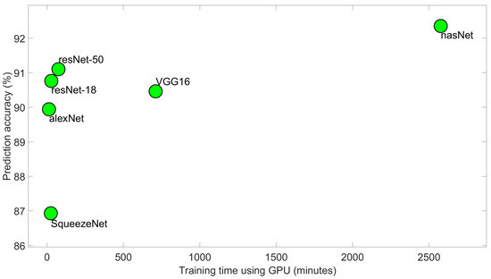
Figure 6.
Network prediction accuracy vs. training time using GPU (NVIDIA(R) GeForce RTX(TM) 3070 Ti) for a mini-batch size of 10 at 50 epochs. Source: [50].
Regarding the RMSE, SqueezeNet resulted in the lowest value, outperforming ResNet-50 by 1.7%, VGG16 by 2.4%, AlexNet by 4.4%, ResNet-18 by 11.7%, and NASNet by 40.4%.
For qualitative evaluation, we plotted the lanes predicted by each network to assess how close these are to the ground truth. Figure 7 shows the lanes predicted by the top performing network, NASNet, along with the ground truth labels. It was evident that the prediction follows the trajectory of the actual lanes, being very close to each other.

Figure 7.
Ground truth labels and predicted lanes for test images using NASNet (mini-batch size of 10 at 50 epochs). Source: [42,95].
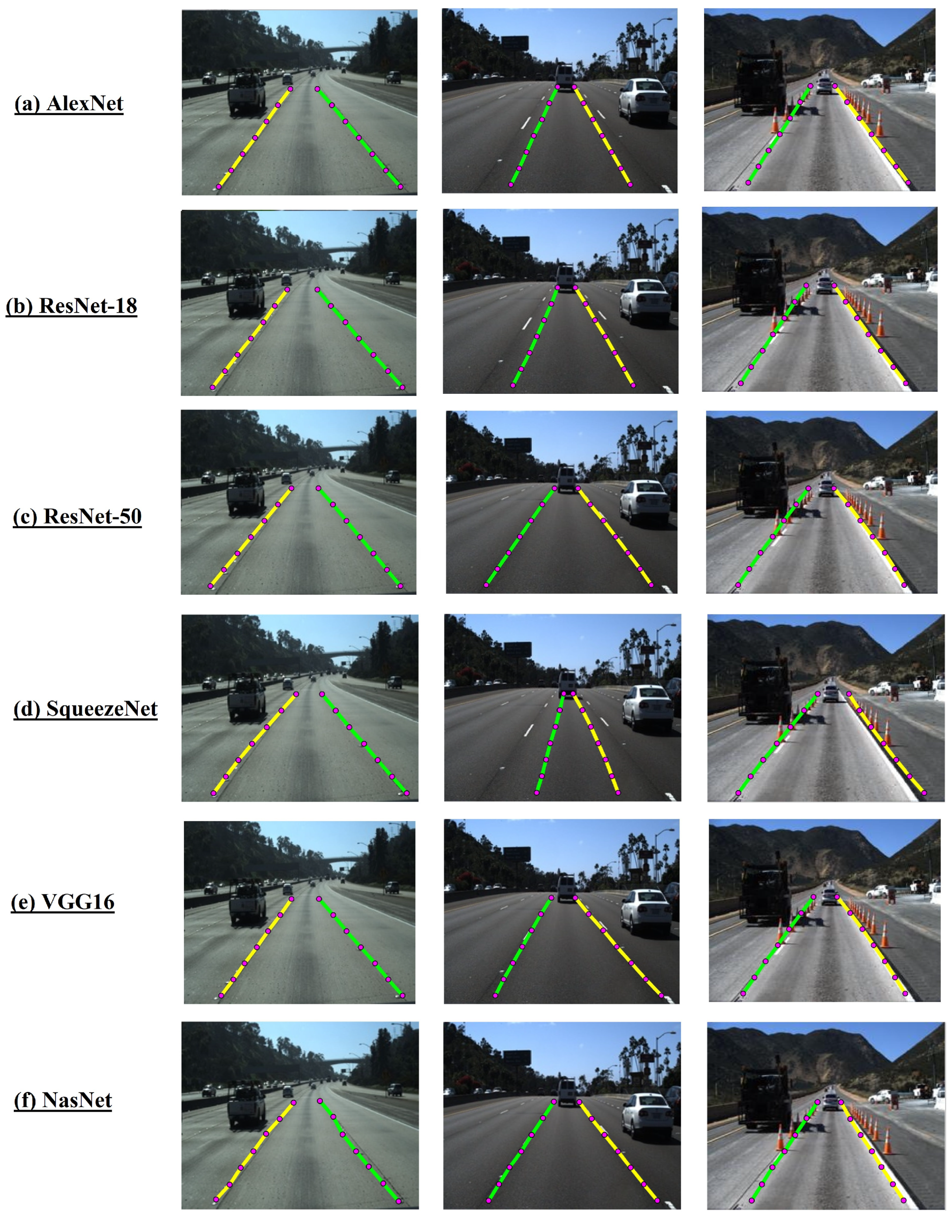
Comparing the predictions of the different networks, we observe in Figure 8 that the points predicted by ResNet-50, VGG16, and NASNet are the closest to the ground truth. Concerning the predictions of AlexNet, ResNet-18, and SqueezeNet, it is observed that the lanes do not vary much from each other. However, for the image in column two, the prediction differs by a medium degree from the ground truth, with SqueezeNet being the furthest from the actual lane. It is unclear which of the two networks, AlexNet or ResNet-18, performs better than the other.
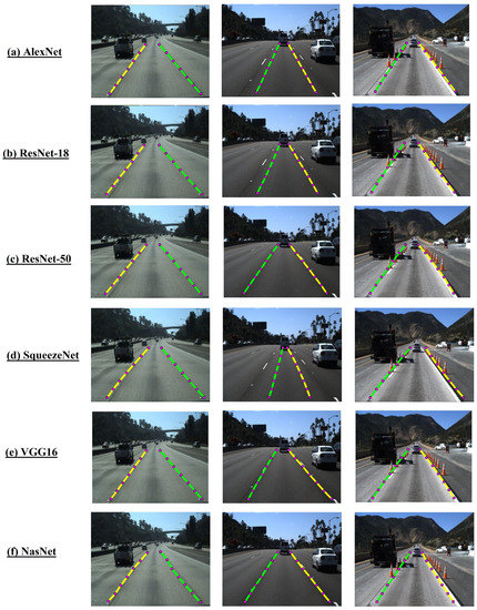
Figure 8.
Lanes predicted for some test images by (a) AlexNet, (b) ResNet-18, (c) ResNet-50, (d) SqueezeNet, (e) VGG16 and (f) NASNet. Source: [42,95].
4.2. Challenging Driving Environment Conditions Results
Because not all networks presented the highest performance with the same combination of hyperparameters, we relied on their convergence for evaluating and comparing performance in different challenging environmental scenarios. Thus, from the hyperparameter selection experiment, we selected the model from each of them that proved to be the best in terms of accuracy and RMSE value. Regarding training time, our study observed that 50 epochs, each with 245 iterations, for a total of 12,250 iterations, was sufficient time for all networks. At that point, the validation error had stabilized around the minimum value with a minor update, and the model had not been overfitted [82,88,96,97]. In Table 3, we present the accuracy results obtained for the challenging driving environmental conditions, and in Table 4, the RMSE results.

Table 3.
Accuracy results obtained for the challenging driving environmental conditions.

Table 4.
RMSE results obtained for the challenging driving environmental conditions.
4.2.1. Daytime Road under Normal Conditions
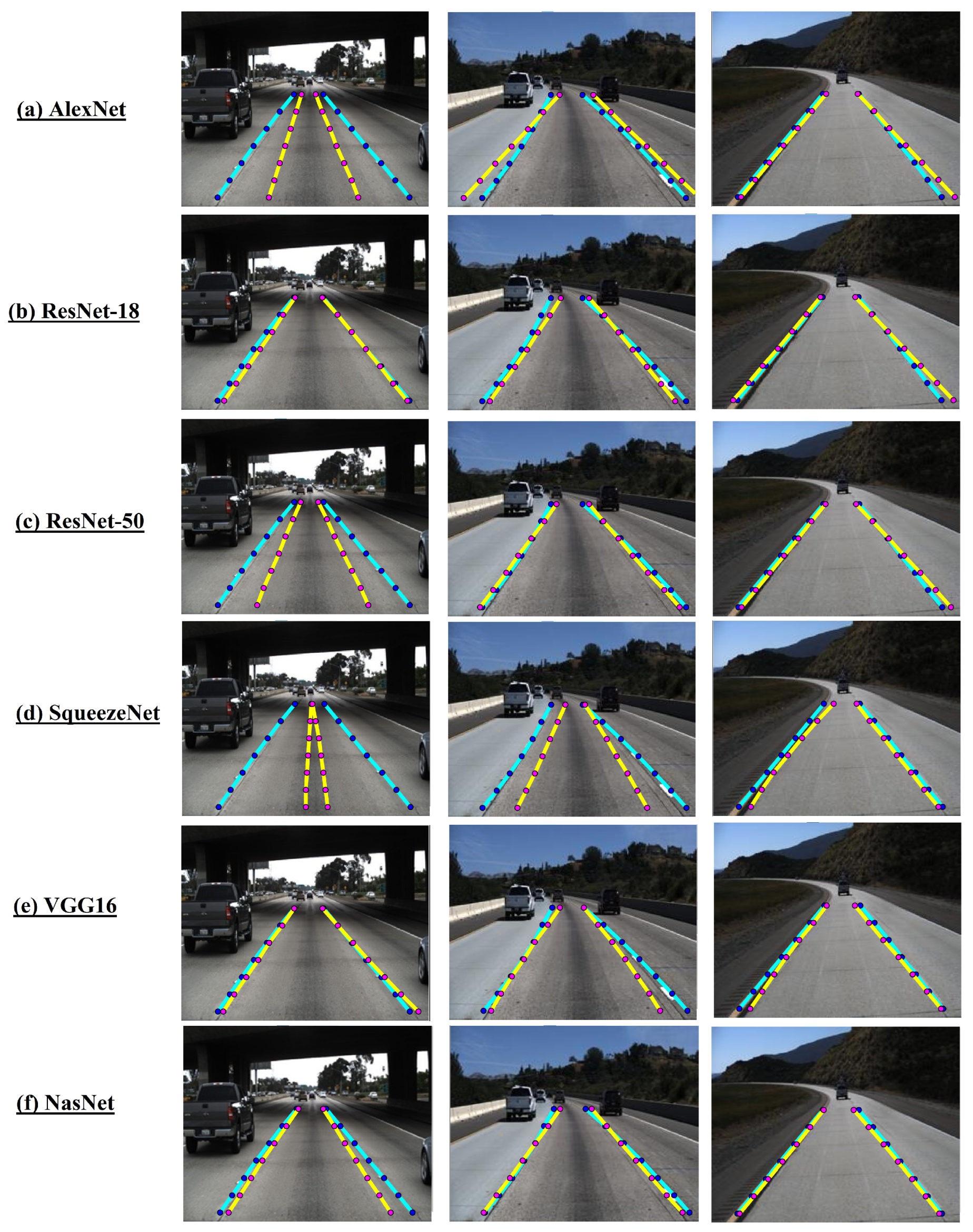
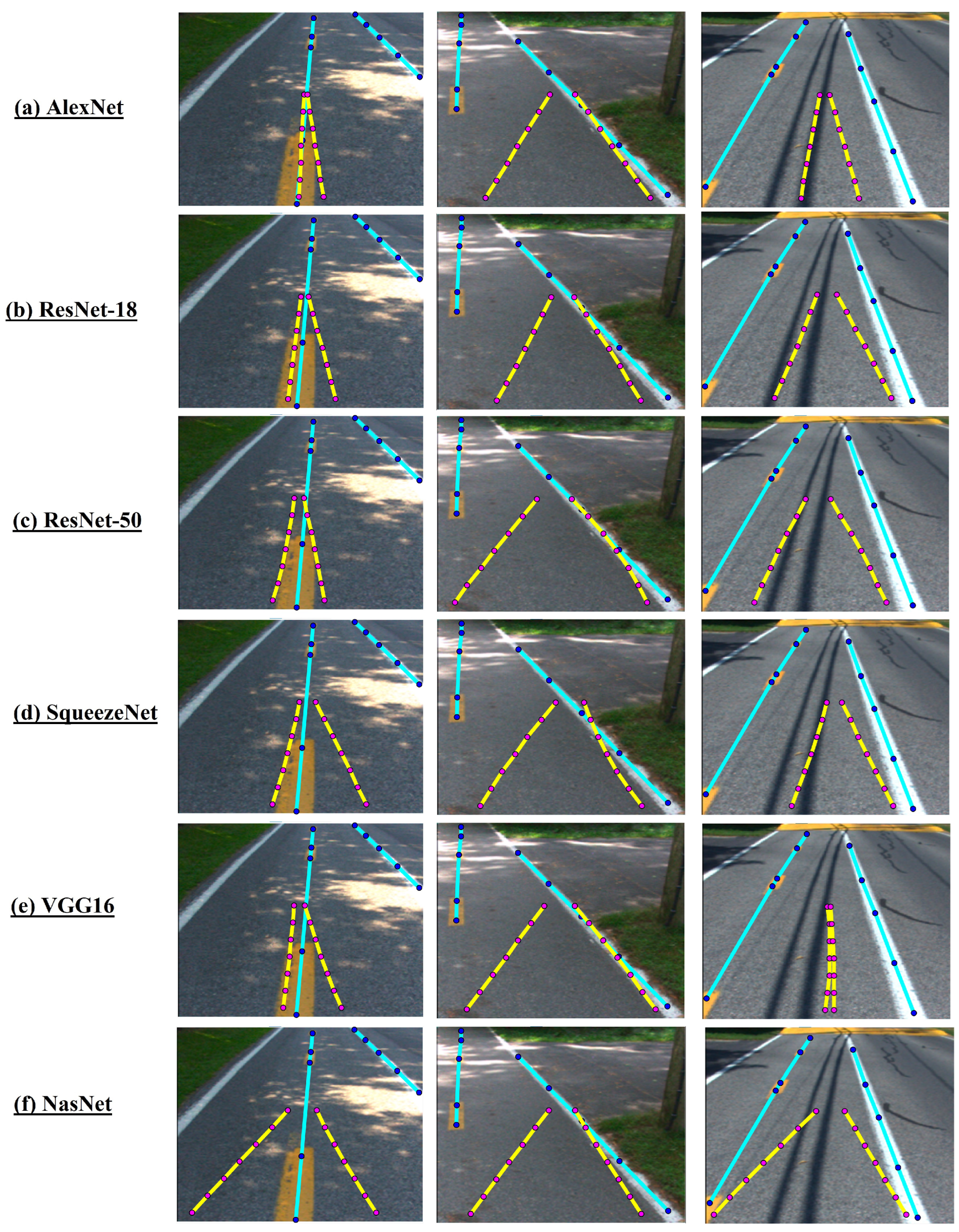
Concerning the predicted lanes plot on the road images under normal conditions, we observed that these are the ones that most closely resemble the ground truth, as shown in Figure 9. Some exceptions include the images in the first column corresponding to AlexNet, ResNet-50, and SqueezeNet. Of the images evaluated, the predictions of NASNet and ResNet-18 for this situation are the closest to the ground truth, whose performances are very similar.
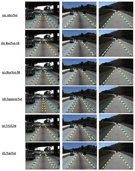
Figure 9.
Lane prediction (yellow/magenta) and ground truth (cyan/blue) for daytime road images under normal conditions using (a) AlexNet, (b) ResNet-18, (c) ResNet-50, (d) SqueezeNet, (e) VGG16, and (f) NASNet. Source: [42,95].
At first glance, it is unclear which is the best performing network among ResNet-18, ResNet-50, NASNet, and VGG16. However, from the calculated accuracy presented in Table 3, it was observed that NASNet was the best performer with 92.07% accuracy, closely followed by ResNet-50 with 90.61% and VGG16 with 90.07%. ResNet-18 achieved an accuracy of 89.07%. Regarding the RMSE values, Table 4, the AlexNet network outperforms VGG16 by 4.13%, ResNet-50 and SqueezeNet by 11.59%, ResNet-18 by 14.63%, and NASNet by 48.59%. The values obtained for this situation are close to those obtained from the training and initial testing of the selected networks. This is because the daytime road scenario under normal conditions resembles the training scenario of the networks.
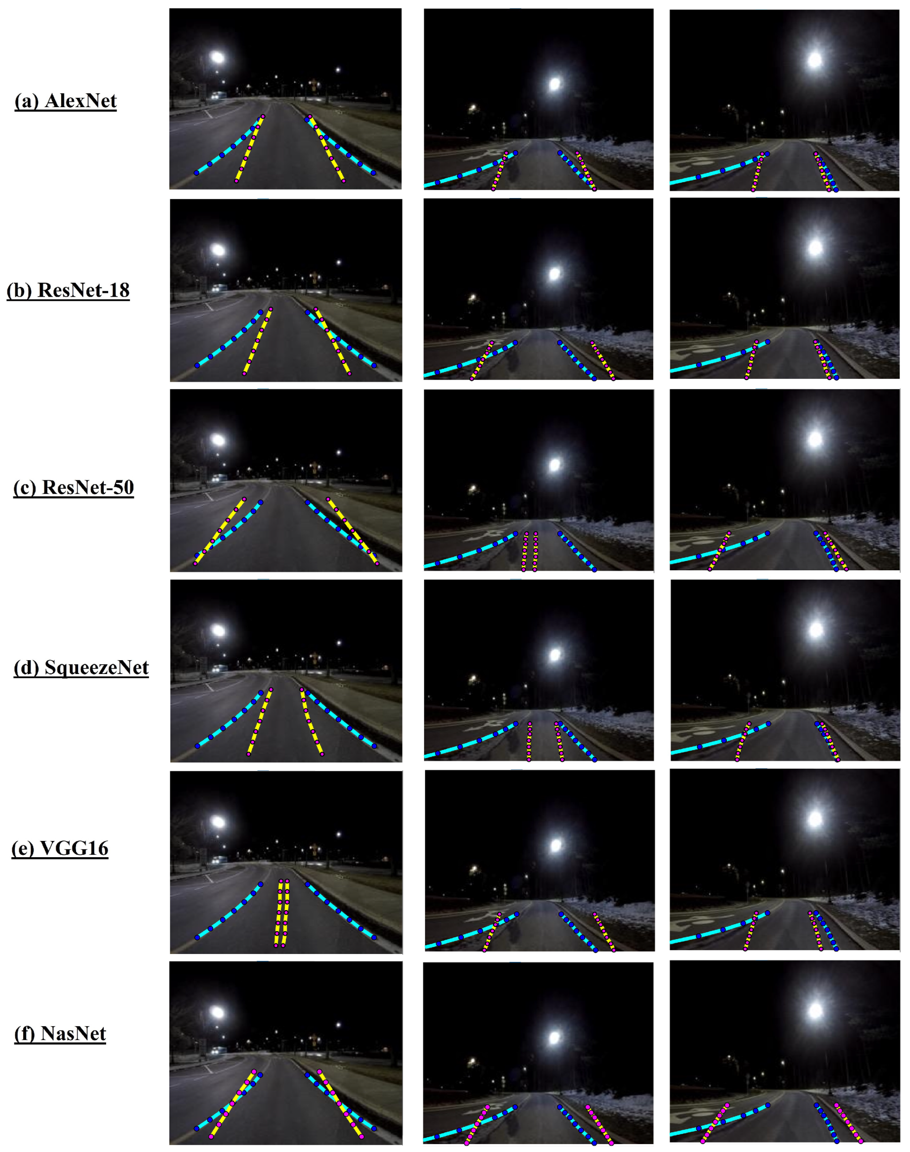
4.2.2. Night Road in Normal Conditions
Of the situations evaluated and the six trained networks, the road situation at night under normal conditions ranked fourth in terms of the highest accuracy and lowest RMSE values. ResNet-50 and AlexNet presented prediction values closer to the ground truth, as corroborated by the accuracy calculation (Table 3) with 52% and 51.43%, respectively. NASNet had the lowest accuracy percentage, 40.39%, despite being the best performer under normal conditions. In terms of RMSE, AlexNet outperforms SqueezeNet by 2.18%, ResNet-18 by 3.7%, VGG16 by 7.3%, ResNet-50 by 13.4%, and NASNet by 49%.
From visual inspection, it can be observed that the networks did not have good results predicting the lanes. They present an intermediate performance compared to the other conditions, as observed in Figure 10.
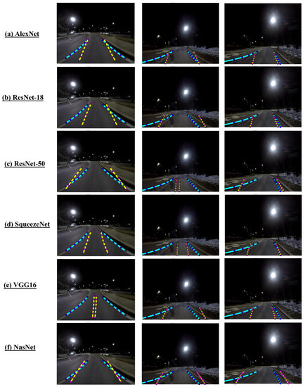
Figure 10.
Nighttime lane prediction (yellow/magenta) and ground truth (cyan/blue) under normal conditions using (a) AlexNet, (b) ResNet-18, (c) ResNet-50, (d) SqueezeNet, (e) VGG16, and (f) NASNet. Source: [95].
When comparing the performance of the networks under normal nighttime road conditions with normal daytime conditions, we observed an average decrease of 40.1% in accuracy. AlexNet had the slightest difference (33.21%) and NASNet the greatest (51.68%) from the value under normal conditions. We note an average increase of 165.3% in RMSE. VGG16 increased the most, with a 179% difference, and ResNet-18 the least, with a 145% difference.
The change in lighting and the shadows created on the road makes it difficult for networks to perform well in this situation.
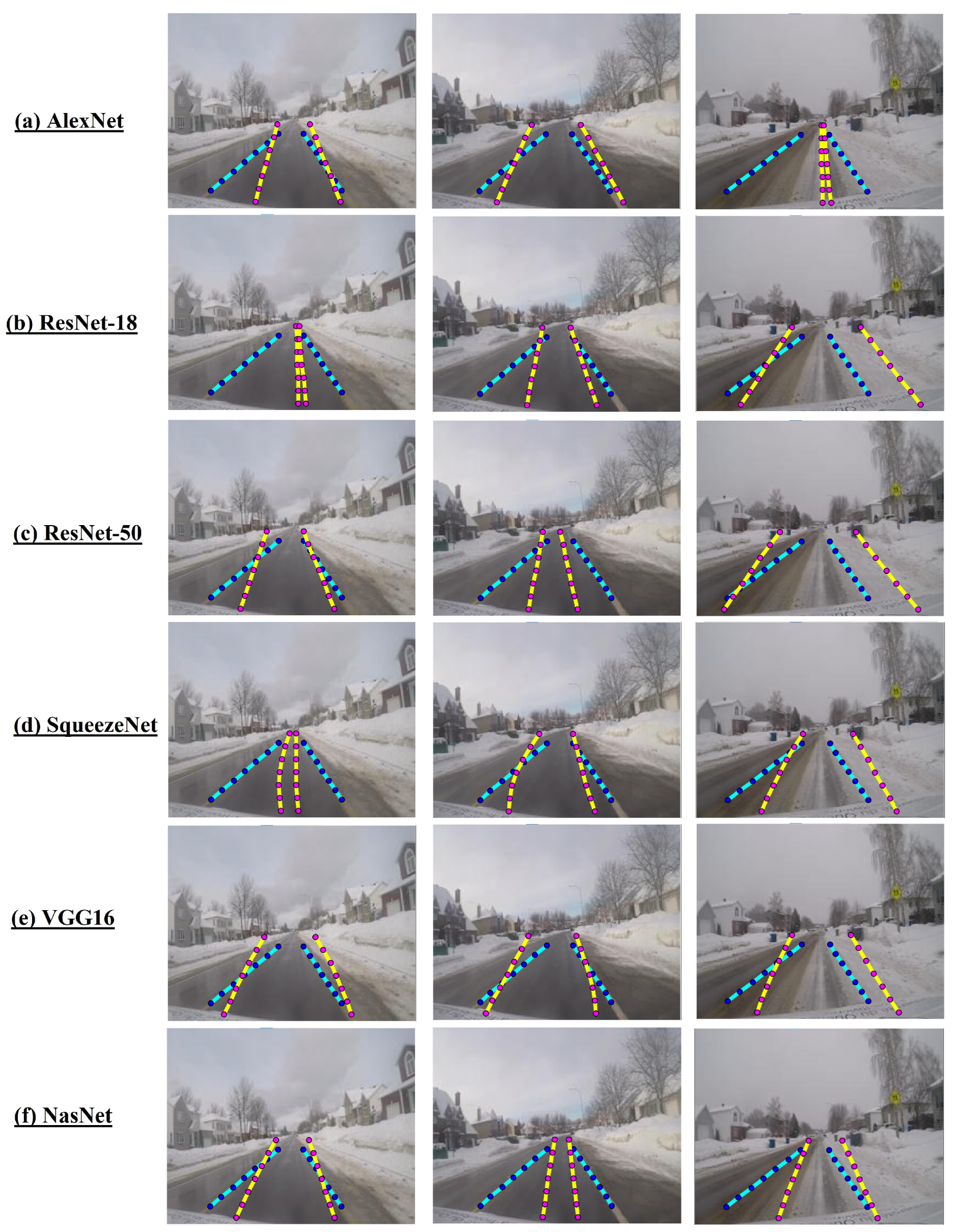
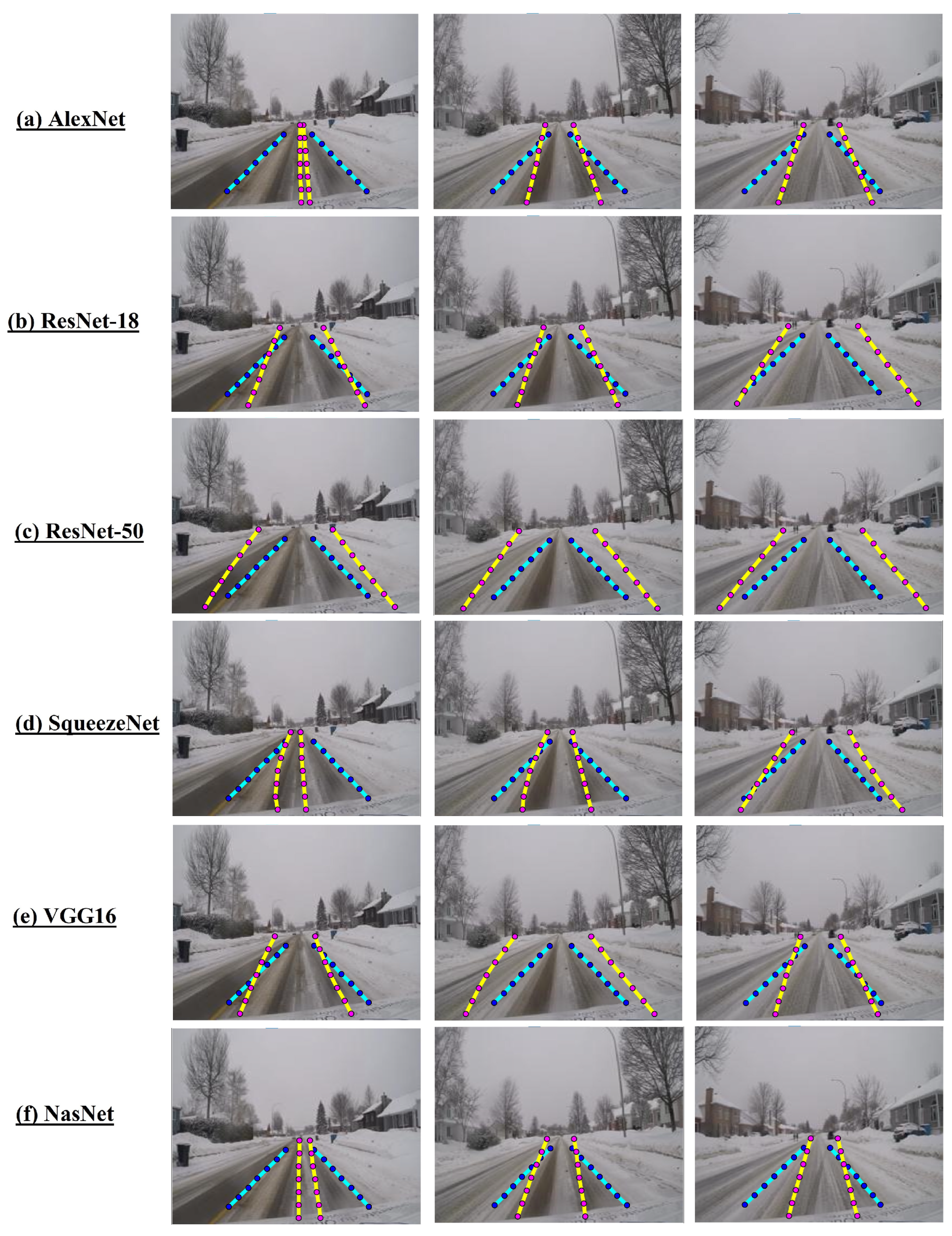
4.2.3. Daytime Road with Light and Moderate Snow
The CNNs in the snowy daytime road scenarios performed better than in the other challenging situations. Their behavior was the closest to the performance in normal daytime conditions.
The network’s performance on the road with light snow was the second best concerning accuracy, with values of 68.25% for ResNet-18, 66.71% for VGG16, 66.57% for AlexNet, 64.18% for SqueezeNet, 63.11% for NASNet and 60.11% for ResNet-50. Comparing this situation with normal road conditions, the decrease in network accuracy was the smallest, with an average decrease of 23.91%. AlexNet presented the slightest difference, 18.07%, and ResNet-50 the largest, 30.5%.
Closely following the performance of the light snow condition is that of the moderate snow situation. ResNet-18 again took first place with 67.04% accuracy. It is followed by VGG16, SqueezeNet, AlexNet, and NASNet, with 64.71%, 63.57%, 62.89%, and 60.82%, respectively. Contrary to the other situations, except for light snow, ResNet-50 ranked last with 56.71%. By comparing this situation with normal road conditions, we noticed an average decrease of 26.1% in the accuracy of the networks. Similar to the light snow situation, AlexNet presented the smallest difference, with 21.75%, and ResNet-50 the largest, with 33.9%.
In contrast to the conditions described above, the ResNet-18 network had the best accuracy for these two daytime snow situations, and the ResNet-50 network had the lowest value.
Regarding the RMSE values, the prediction for the daytime road with light snow was the second lowest value, with AlexNet outperforming SqueezeNet by 2.2%, VGG16 by 15%, ResNet-18 by 16.4%, ResNet-50 by 34.4% and NASNet by 70.7%. The moderate snow condition RMSE value followed that of the light snow condition, with AlexNet again beating SqueezeNet by 8.5%, ResNet-18 by 16.6%, VGG16 by 21.2%, ResNet-50 by 37.3%, and NASNet by 61.6%. The average increase in RMSE of the light snow and moderate snow conditions to normal daytime road conditions was 87.6% and 95.7%, respectively, the lowest increases of all conditions evaluated.
From visual inspection, it can be observed that the networks have less trouble identifying lane lines for the light snow situation (Figure 11) compared to the moderate snow situation (Figure 12). This difference is due to the low lane visibility caused by the increased snow on the road. In both situations, the coordinates of the predicted points differ barely from the ground truth. However, we note that the networks confuse the proper lane lines with some false lines created by the accumulation of ice and snow on the road. Despite this confusion, we note that these points try to follow the shape of the lanes.
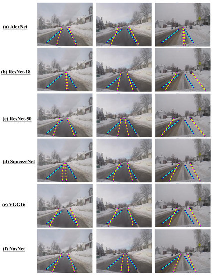
Figure 11.
Predicted lanes (yellow/magenta) and ground truth (cyan/blue) for daytime road with light snow using (a) AlexNet, (b) ResNet-18, (c) ResNet-50, (d) SqueezeNet, (e) VGG16, and (f) NASNet. Source: [95].
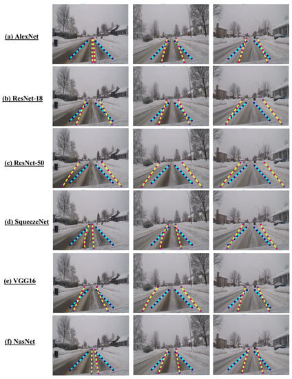
Figure 12.
Predicted lanes (yellow/magenta) and ground truth (cyan/blue) for daytime road with moderate snow using (a) AlexNet, (b) ResNet-18, (c) ResNet-50, (d) SqueezeNet, (e) VGG16, and (f) NASNet. Source: [95].
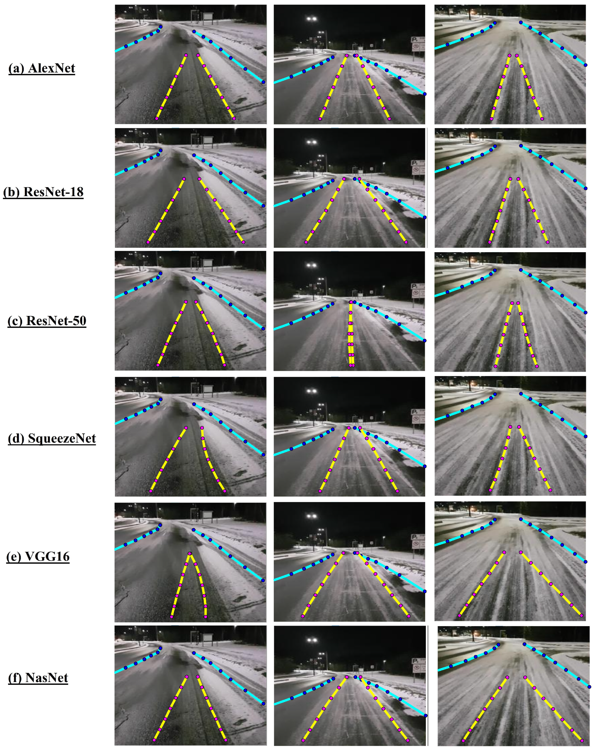
4.2.4. Night Road with Snow
Of the challenging conditions evaluated, the snowy night road had the lowest performance in both accuracy and RMSE values. There was a significant decrease in performance compared to normal driving conditions, with 75.2% less accuracy on average and a significant increase in RMSE of 301.12%, the highest of all situations evaluated.
Assessing networks’ performance under this condition, AlexNet was the worst performer in terms of accuracy with a value of 11.96%. NASNet followed closely with 13.07%, as did SqueezeNet with 13.71%. The accuracy values of ResNet-18 and VGG16 differ by 0.43%, with the former being the highest performing for this condition. Contrary to the accuracy results, AlexNet outperformed the other networks, having a lower RMSE than ResNet-50, VGG16, SqueezeNet, ResNet-18, and NASNet by 4.9%, 5%, 5.89%, 7.9%, and 56.5% respectively.
We observe in the images if the predicted lanes and ground truth in Figure 13 that the networks confuse the proper lane with the fictitious lines created by snow and ice on the road. The existing lane lines have poor visibility as these same elements cover them. This behavior is the same as that on the daytime road in moderate snow. Nevertheless, it is noted in most images that the predicted points follow the shape of the lane even if their coordinates are far from the true ones, as in the conditions described above.
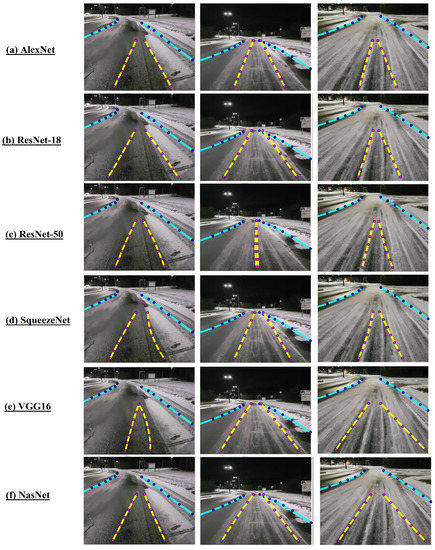
Figure 13.
Predicted lanes (yellow/magenta) and ground truth (cyan/blue) for the nighttime snowy road using (a) AlexNet, (b) ResNet-18, (c) ResNet-50, (d) SqueezeNet, (e) VGG16, and (f) NASNet. Source: [95].
The performance of the networks decreases drastically with the combination of illumination changes, decreased contrast, poor lane visibility due to snow and ice accumulation, and the creation of false lines on the road. The above is because these deep learning methods cannot adequately adjust to these situations outside the training set because the stochastic distributions of their features changes.
4.2.5. Road with Occluded Areas
The performance regarding quantitative and qualitative variables evaluated for the road with occluded areas was also among the lowest. This can be seen in Figure 14, in Table 3 and Table 4.
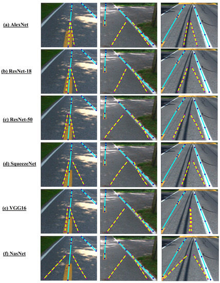
Figure 14.
Predicted lanes (yellow-magenta) and ground truth (cyan-blue) for the road with occluded areas using (a) AlexNet, (b) ResNet-18, (c) ResNet-50, (d) SqueezeNet, (e) VGG16 and (f) NASNet. Source: [95].
In many of the images evaluated, we observe that the coordinates of the predicted points of the lanes with continuous white lines are closer to the ground truth. This can be seen in the images of the second and third columns of Figure 14, where the points are closer to the right lane. The preceding might suggest that the networks better detect lane lines that are white and continuous. However, this is not the case in situations such as daytime roads under normal conditions. In these, the networks make good predictions for lanes with dashed white lines or solid yellow lines.
Regarding accuracy and RMSE values, the networks generally did not perform well. They showed a decrease in the accuracy percentage of 55.95% compared to the values achieved with the normal daytime images. The RMSE results increased significantly by 230.2%. Comparing the networks individually, ResNet-18 had the highest accuracy percentage with a value of 39.46%. It outperformed ResNet-50 by 1.82%, AlexNet by 2.28%, VGG16 by 8.78%, SqueezeNet by 11.1%, and NASNet by 16.07%. In terms of RMSE, ResNet-50 and AlexNet surpassed ResNet-18 by 4.1%, VGG16 by 20.9%, SqueezeNet by 22.2%, and NASNet by 80.7%.
Analogous to the snowy road scenarios, for this situation the networks confused the right lane lines with false lines created by the shadows of elements close to the road or by defects on the pavement.
5. Discussion
With this work, we experimentally analyze the extent to which different challenging environmental driving conditions affect the performance of deep learning methods. We compare the performance of six varied and commonly used network architectures in lane detection. For reference, the different methods were applied to normal daytime driving conditions and compared with the performance obtained under challenging situations.
From a broad point of view, it is observed that the networks could not transfer the performance obtained under normal daytime conditions to the other situations. They showed a performance decrease, with a significant drop in the accuracy percentage and an increase in the RMSE for all cases.
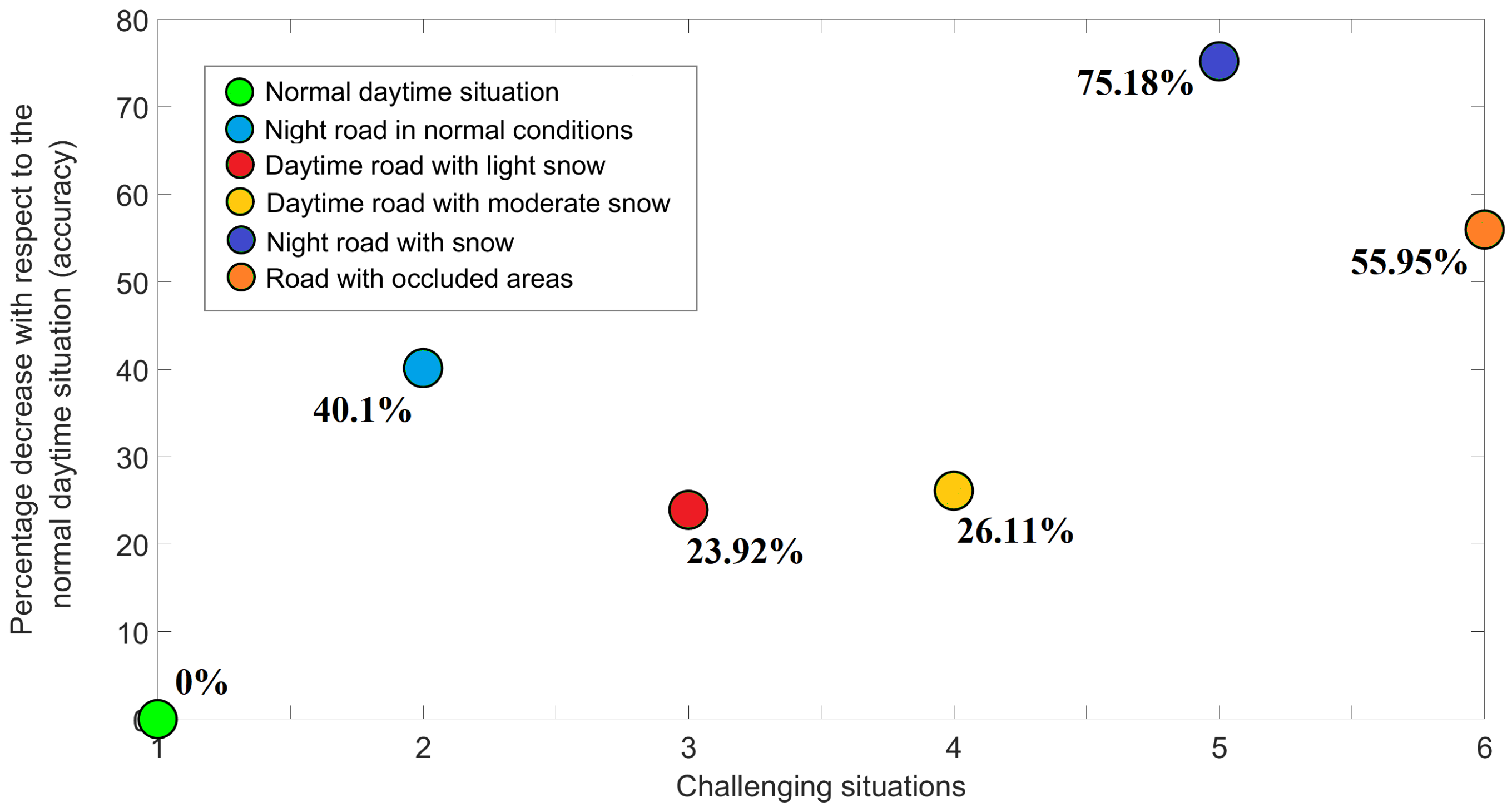
Table 5 and Table 6 show this decay in terms of accuracy and RMSE values for each situation and each network evaluated. The least challenging situation for the architectures was the daytime situation with light snow, followed closely by the daytime situation with moderate snow, although the percentages decrease were 23.9% and 26.11%, respectively. As for the RMSE values, the increases presented for these situations were 87.64% and 95.67%, respectively. The road with occluded areas and the night road with snow were the most challenging for the networks. They presented drops in prediction accuracy of 55.95% and 75.18%, respectively, and increases in the RMSE value of 230.19% and 301.12%, respectively. This behavior can be seen in Figure 15.

Table 5.
Percentage decrease in the accuracy of networks under challenging conditions with respect to values obtained under normal daytime conditions.

Table 6.
Percentage increase in the RMSE value of the networks under challenging conditions with respect to values obtained under normal daytime conditions.
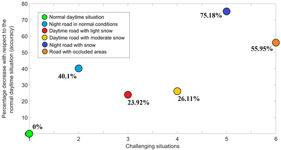
Figure 15.
Percentage decrease in networks’ accuracy under challenging conditions with respect to values obtained under normal daytime conditions.
The network that was least affected by all situations was AlexNet, with a minor difference in accuracy percentages. Although the differences in RMSE values concerning their performance under normal conditions were not the lowest, AlexNet was the network that obtained the lowest RMSE values in each situation, as shown in Table 4. The networks that suffered the most in all situations were NASNet and ResNet-50, in contrast to their performance in normal daytime conditions, where they obtained the best prediction accuracy results.
As for the punctual performance of the networks with each challenging situation, we note that ResNet-18 had the best percentage of prediction accuracy. NASNet and ResNet-50 had the lowest percentages.
The fact that the performance of the networks under normal daytime conditions could not be satisfactorily transferred to slightly different situations from the training scenarios demonstrates a generalization problem.
Lane non-visibility, illumination changes, false lane lines, and road contrast variations modify the images’ features and add noise. This change in the features modifies the stochastic feature distributions, making them different from the distributions of the features corresponding to normal daytime driving conditions. This difference causes a decrease in the performance of deep learning methods and a drastic reduction in accuracy.
Generally speaking, it is said that the performance of all deep learning-based methods decreases, regardless of their nature (segmentation, regression, classification), because they use feature extractors. Any statistical change in the input data or noise affecting the spatial features will make them vulnerable. It is essential to consider these various road conditions when training the networks to improve the robustness and inclusiveness of the lane detection methods, thus avoiding a decrease in network performance.
In the broader context of autonomous navigation, this drop in performance accuracy impacts both vehicle safety and energy consumption. The vehicle can become a potential obstacle and cause severe road accidents if it cannot detect the lane. The car will not be able to stay in it and may steer away [98]. Likewise, it will not be able to change lanes properly. Any improper planning and execution of movement on the road can lead to an accident, such as a rollover accident or collision with another vehicle, a stationary object, or pedestrians [99]. Similarly, the energy budget will be affected by causing the navigation system to move the vehicle back to its correct lane. It is better to try to stay in the lane than to try to return after leaving it. Significant effort must be made to optimize these autonomous driving components and ensure their correct operation in different driving conditions for these energy and safety reasons.
Finding alternative ways to help mitigate performance degradation in challenging environments is essential. In the study by Boisclair et al. [100], the fusion of different image modalities into a single network is proposed as a solution to the performance degradation of neural networks under adverse weather conditions such as snowfall or rainfall. The authors adopt a parallel multimodal network that receives any image modality. The authors indicate that depth images, which do not need color information, or thermal photos, which are not affected by precipitation or fog, show good performance. In the article of Sattar and Mo [101], image overlay and alignment are used to find the lane position on roads where the lane is not fully visible. It uses vehicle position information and camera orientation to locate and access alternative images of the visible road and attempt detection on one of these. This research uses feature-based matching to find the corresponding image feature points between the evaluated image and the visual database image most closely resembles it. From the common regions found, pixel-based matching was used to enhance the alignment. In the work of Sajeed et al. [98], a geographic information system (GIS) and an inertial navigation system are incorporated to locate the vehicle on the road without relying on the visibility of the lane markers. This overcomes the limitations of the vision camera, the LiDAR, and the GPS. The OpenStreetMap (OSM) map database was used to obtain the geospatial data on street attributes and geometry. The authors extracted road segments with geographic latitude–longitude points located at the center of the road.
Other possible solutions to the decrease in lane detection accuracy under challenging conditions are proposed in the future work section, considering the above alternatives.
6. Conclusions and Future Work
In this paper, we presented an experimental analysis of the impact of several challenging environmental driving conditions on the performance of regression-based neural networks for lane detection. Six varied and commonly used architectures (alexNet, resNet-18, resNet-50, squeezeNet, VGG16, and NASNet) were compared under challenging and normal environmental conditions.
Based on the evaluation and analysis of the benchmark, we found that all networks failed to extend the performance achieved successfully under normal conditions. The daytime snowy road conditions affected performance to a lesser extent than the others. The nighttime snowy road affected it the most. The accuracy percentage decreased considerably in all cases, and the RMSE increased drastically.
Overall, we confirm that scenarios where road conditions have little or no similarity to what has been previously learned pose challenges for deep learning algorithms. The stochastic distributions of the environment features vary with the presence of different factors such as noise, snow, or shadows, preventing networks from adapting adequately, as they base their predictions on the extraction of static features and dependencies.
In future work, it is proposed to include different sets of road images under various environmental conditions in training deep learning-based methods. The above is formulated to test if the networks can delimit the driving area by matching the common static features of the environment between similar images, such as trees or buildings. With this, we will try to solve the generalization problem and make our methods more stable and reliable. Likewise, a fusion of sensors (radar, thermal camera, visible camera, and LiDAR) is proposed to complement the previous point, thus having more information about the environment and finding more common static features with greater reliability. Another suggested option is to generate lane lines virtually by applying augmented reality to road images under adverse conditions. Visual and geolocation information from road images in visible and non-visible situations would be used to infer where the lane is located on roads with snow accumulation. The visual information encompasses the static reference features in the environment, which could be extracted using the encoding portion of an autoencoder. Additionally, using the approach of Sajeed et al. [98], the position of the lane lines could be inferred, and a virtual lane could be generated. Geographic latitude–longitude points located at the center of the road, extracted from the OSM database, would be used.
Author Contributions
Conceptualization, S.K. and A.U.-Q.; methodology, T.O.-S., S.K. and M.Z.A.; software, T.O.-S.; validation, T.O.-S., S.K. and M.Z.A.; formal analysis, T.O.-S.; investigation, T.O.-S., S.K. and M.Z.A.; resources, S.K. and A.A.; writing—original draft preparation, T.O.-S.; writing—review and editing, S.K., M.Z.A., A.U.-Q. and A.A.; supervision, S.K., A.U.-Q., P.P.-R. and F.G.-V. All authors have read and agreed to the published version of the manuscript.
Funding
This work was supported by the Natural Sciences and Engineering Research Council of Canada, and the Canada Research Chair.
Institutional Review Board Statement
Not applicable.
Informed Consent Statement
Not applicable.
Data Availability Statement
For training the networks chosen for this study, we used the open-access dataset introduced by TuSimple in the TuSimple benchmark [42]. The dataset of images with challenging weather conditions is available on request from the corresponding author.
Acknowledgments
Authors would like to thank the Université du Québec à Trois-Rivières and the Institut de recherche sur l’hydrogène for their collaboration and assistance.
Conflicts of Interest
The authors declare no conflict of interest and the funders had no role in the design of the study; in the collection, analyses, or interpretation of data; in the writing of the manuscript, or in the decision to publish the results.
Abbreviations
The following abbreviations are used in this manuscript:
| ACP | Artificial Society, Computational experiments, and Parallel execution |
| AVs | Autonomous vehicles |
| CNNs | Convolutional neural networks |
| FCNs | Fully convolutional neural networks |
| GPS | Global Positioning System |
| ILSVRC | ImageNet Large-Scale Visual Recognition Challenge |
| INS | Inertial navigation system |
| IoU | Intersection over Union |
| LDP | Lane departure prevention |
| LDW | Lane departure warning |
| LiDAR | Light Detection and Ranging |
| LSTM | Long short-term memory |
| ReLU | Rectified Linear Unit |
| RMSE | Root mean square error |
| RNNs | Recurrent neural networks |
| SAD | Self Attention Distillation |
| SGDM | Stochastic gradient descent with momentum |
| YOLO | You Only Look Once |
References
- Lederman, J.; Bronston, S. Biden Plan Seeks to Jumpstart Rollout of Electric Vehicle Charging Stations. 2021. Available online: https://www.nbcnews.com/politics/white-house/biden-administration-releasing-strategy-building-u-s-electric-vehicle-charging-n1285813 (accessed on 15 December 2021).
- Motavalli, J. Every Automaker’s EV Plans through 2035 and beyond. 2021. Available online: https://www.forbes.com/wheels/news/automaker-ev-plans/ (accessed on 15 December 2021).
- Ratzlaff, B. Canada Aiming to Shift to All Zero-Emission Electric Vehicles by 2035: Federal Government. 2021. Available online: https://globalnews.ca/news/8039066/canada-zero-emission-electric-vehicles/ (accessed on 15 December 2021).
- Ministerio de Energía de Chile. Vehículos de Conducción Autónoma. 2021. Available online: https://energia.gob.cl/electromovilidad/modelos-de-negocios/conduccion-autonoma-para-vehiculos-electricos (accessed on 14 December 2021).
- Penmetsa, P.; Hudnall, M.; Nambisan, S. Potential safety benefits of lane departure prevention technology. IATSS Res. 2019, 43, 21–26. [Google Scholar] [CrossRef]
- Mohammed, A.S.; Amamou, A.; Ayevide, F.K.; Kelouwani, S.; Agbossou, K.; Zioui, N. The Perception System of Intelligent Ground Vehicles in All Weather Conditions: A Systematic Literature Review. Sensors 2020, 20, 6532. [Google Scholar] [CrossRef] [PubMed]
- Tang, J.; Li, S.; Liu, P. A review of lane detection methods based on deep learning. Pattern Recognit. 2021, 111, 107623. [Google Scholar] [CrossRef]
- Alam, M.Z.; Boisclair, J.; Kelouwani, S. Learning Light fields for improved lane detection. 2021; Unpublished results. [Google Scholar]
- Zou, Q.; Jiang, H.; Dai, Q.; Yue, Y.; Chen, L.; Wang, Q. Robust Lane Detection From Continuous Driving Scenes Using Deep Neural Networks. IEEE Trans. Veh. Technol. 2020, 69, 41–54. [Google Scholar] [CrossRef]
- Narote, S.P.; Bhujbal, P.N.; Narote, A.S.; Dhane, D.M. A review of recent advances in lane detection and departure warning system. Pattern Recognit. 2018, 73, 216–234. [Google Scholar] [CrossRef]
- Ghani, H.A.; Besar, R.; Sani, Z.M.; Kamaruddin, M.N.; Syahali, S.; Daud, A.M.; Martin, A. Advances in lane marking detection algorithms for all-weather conditions. Int. J. Electr. Comput. Eng. 2021, 11, 3365–3373. [Google Scholar] [CrossRef]
- Xing, Y.; Lv, C.; Chen, L.; Wang, H.; Wang, H.; Cao, D.; Velenis, E.; Wang, F.Y. Advances in Vision-Based Lane Detection: Algorithms, Integration, Assessment, and Perspectives on ACP-Based Parallel Vision. IEEE/CAA J. Autom. Sin. 2018, 5, 645–661. [Google Scholar] [CrossRef]
- Aly, M. Real time detection of lane markers in urban streets. In Proceedings of the 2008 IEEE Intelligent Vehicles Symposium, Eindhoven, The Netherlands, 4–6 June 2008; pp. 7–12. [Google Scholar] [CrossRef]
- Jung, J.; Bae, S.H. Real-Time Road Lane Detection in Urban Areas Using LiDAR Data. Electronics 2018, 7, 276. [Google Scholar] [CrossRef]
- Neven, D.; Brabandere, B.D.; Georgoulis, S.; Proesmans, M.; Gool, L.V. Towards End-to-End Lane Detection: An Instance Segmentation Approach. In Proceedings of the 2018 IEEE Intelligent Vehicles Symposium (IV), Suzhou, China, 26–30 June 2018; pp. 286–291. [Google Scholar] [CrossRef]
- Kim, J.; Park, C. End-to-end ego lane estimation based on sequential transfer learning for self-driving cars. In Proceedings of the IEEE Conference on Computer Vision and Pattern Recognition (CVPR) Workshops, Honolulu, HI, USA, 21–26 July 2017; pp. 30–38. [Google Scholar]
- Li, J.; Mei, X.; Prokhorov, D.; Tao, D. Deep Neural Network for Structural Prediction and Lane Detection in Traffic Scene. IEEE Trans. Neural Networks Learn. Syst. 2017, 28, 690–703. [Google Scholar] [CrossRef]
- Ko, Y.; Lee, Y.; Azam, S.; Munir, F.; Jeon, M.; Pedrycz, W. Key Points Estimation and Point Instance Segmentation Approach for Lane Detection. IEEE Trans. Intell. Transp. Syst. 2020, 1–10. [Google Scholar] [CrossRef]
- Ali, A.A.; Hussein, H.A. Real-time lane markings recognition based on seed-fill algorithm. In Proceedings of the International Conference on Information and Communication Technology, Kuala Lumpur, Malaysia, 24–26 July 2019; pp. 190–195. [Google Scholar]
- Pizzati, F.; Allodi, M.; Barrera, A.; García, F. Lane Detection and Classification Using Cascaded CNNs. In Proceedings of the Computer Aided Systems Theory—EUROCAST 2019, Las Palmas de Gran Canaria, Spain, 17–22 February 2019; Moreno-Díaz, R., Pichler, F., Quesada-Arencibia, A., Eds.; Springer International Publishing: Cham, Switzerland, 2020; pp. 95–103. [Google Scholar] [CrossRef]
- Khairdoost, N.; Beauchemin, S.S.; Bauer, M.A. Road Lane Detection and Classification in Urban and Suburban Areas based on CNNs. In Proceedings of the VISIGRAPP (5: VISAPP), Online Streaming, 8–10 February 2021; pp. 450–457. [Google Scholar]
- Chougule, S.; Koznek, N.; Ismail, A.; Adam, G.; Narayan, V.; Schulze, M. Reliable multilane detection and classification by utilizing CNN as a regression network. In Proceedings of the European Conference on Computer Vision (ECCV) Workshops, Munich, Germany, 8–14 September 2018. [Google Scholar]
- Ding, L.; Zhang, H.; Xiao, J.; Shu, C.; Lu, S. A lane detection method based on semantic segmentation. Comput. Model. Eng. Sci. 2020, 122, 1039–1053. [Google Scholar] [CrossRef]
- Lu, S.; Luo, Z.; Gao, F.; Liu, M.; Chang, K.; Piao, C. A Fast and Robust Lane Detection Method Based on Semantic Segmentation and Optical Flow Estimation. Sensors 2021, 21, 400. [Google Scholar] [CrossRef] [PubMed]
- Pan, X.; Shi, J.; Luo, P.; Wang, X.; Tang, X. Spatial As Deep: Spatial CNN for Traffic Scene Understanding. In Proceedings of the AAAI Conference on Artificial Intelligence, New Orleans, LA, USA, 2–7 February 2018; Volume 32. [Google Scholar]
- Cao, J.; Song, C.; Song, S.; Xiao, F.; Peng, S. Lane detection algorithm for intelligent vehicles in complex road conditions and dynamic environments. Sensors 2019, 19, 3166. [Google Scholar] [CrossRef] [PubMed]
- ViewNext. El Transfer Learning y las Redes Convolucionales. 2020. Available online: https://www.viewnext.com/transfer-learning-y-redes-convolucionales/ (accessed on 10 April 2021).
- Costa, P. Transfer Learning ¿qué es y Para Que Sirve? 2019. Available online: https://pochocosta.com/podcast/transfer-learning-que-es-y-para-que-sirve/ (accessed on 10 April 2021).
- Zhang, X.; Yang, W.; Tang, X.; Liu, J. A Fast Learning Method for Accurate and Robust Lane Detection Using Two-Stage Feature Extraction with YOLO v3. Sensors 2018, 18, 4308. [Google Scholar] [CrossRef]
- Hou, Y.; Ma, Z.; Liu, C.; Loy, C.C. Learning Lightweight Lane Detection CNNs by Self Attention Distillation. In Proceedings of the IEEE/CVF International Conference on Computer Vision (ICCV), Seoul, Korea, 27 October–2 November 2019; pp. 1013–1021. [Google Scholar] [CrossRef]
- Nehemiah, A. Deep Learning for Automated Driving (Part 2)—Lane Detection. 2017. Available online: https://blogs.mathworks.com/deep-learning/2017/11/17/deep-learning-for-automated-driving-part-2-lane-detection/ (accessed on 15 April 2021).
- Ekşi, O.T.; Gökmen, G. Comparing of Some Convolutional Neural Network (CNN) Architectures for Lane Detection. Balk. J. Electr. Comput. Eng. 2020, 8, 314–319. [Google Scholar] [CrossRef]
- Yang, D.; Bao, W.; Zheng, K. Lane Detection of Smart Car based on Deep Learning. J. Phys. Conf. Ser. 2021, 1873, 012068. [Google Scholar] [CrossRef]
- Minoot7. Lane Detection with Deep Learning Using PINet Model and Tusimple Dataset. 2020. Available online: https://github.com/minoot7/Lane-Detection-Transfer-Learning (accessed on 2 May 2021).
- Olah, C. Understanding LSTM Networks. 2015. Available online: http://colah.github.io/posts/2015-08-Understanding-LSTMs/ (accessed on 3 May 2022).
- Kortli, Y.; Gabsi, S.; Voon, L.F.L.Y.; Jridi, M.; Merzougui, M.; Atri, M. Deep embedded hybrid CNN–LSTM network for lane detection on NVIDIA Jetson Xavier NX. Knowl.-Based Syst. 2022, 240, 107941. [Google Scholar] [CrossRef]
- Wu, J.; Cui, H.; Dahnoun, N. Gradient Map Based Lane Detection Using CNN and RNN. In Proceedings of the 2020 22th International Conference on Digital Signal Processing and Its Applications (DSPA), Moscow, Russia, 25–27 March 2020; pp. 1–5. [Google Scholar] [CrossRef]
- Microsoft. Aprendizaje Profundo Frente a Aprendizaje Automático en Azure Machine Learning. 2022. Available online: https://docs.microsoft.com/es-es/azure/machine-learning/concept-deep-learning-vs-machine-learning (accessed on 19 May 2022).
- Transformador (Modelo de Aprendizaje Automático). 2021. Available online: https://hmong.es/wiki/Transformer_(machine_learning) (accessed on 19 May 2022).
- Liu, R.; Yuan, Z.; Liu, T.; Xiong, Z. End-to-end lane shape prediction with transformers. In Proceedings of the IEEE/CVF Winter Conference on Applications of Computer Vision, Waikoloa, HI, USA, 3–8 January 2021; pp. 3694–3702. [Google Scholar]
- Han, J.; Deng, X.; Cai, X.; Yang, Z.; Xu, H.; Xu, C.; Liang, X. Laneformer: Object-aware Row-Column Transformers for Lane Detection. arXiv 2022, arXiv:2203.09830. [Google Scholar] [CrossRef]
- Tomatosliu; KevinWangTHU; Li, C. TuSimple Lane Detection Challenge—Data Licensed under CC-BY-SA. 2017. Available online: https://github.com/TuSimple/tusimple-benchmark/tree/master/doc/ (accessed on 10 April 2021).
- Siddiqui, K.A. To What Resolution Should I Resize My Images to Use as Training Dataset for Deep Learning? 2018. Available online: https://qr.ae/pvUCU0 (accessed on 10 April 2021).
- Hashemi, M. Enlarging smaller images before inputting into convolutional neural network: Zero-padding vs. interpolation. J. Big Data 2019, 6, 98. [Google Scholar] [CrossRef]
- MATLAB. MATLAB and Ground Truth Labeler App Release 2017a; The MathWorks Inc.: Natick, MA, USA, 2017. [Google Scholar]
- MATLAB. MATLAB and Automated Driving System Toolbox Release 2021a; The MathWorks Inc.: Natick, MA, USA, 2021. [Google Scholar]
- MATLAB. Get Started with the Image Labeler; The MathWorks Inc.: Natick, MA, USA, 2017; Available online: https://www.mathworks.com/help/vision/ug/get-started-with-the-image-labeler.html (accessed on 15 April 2021).
- Yang, W.; Zhang, X.; Lei, Q.; Shen, D.; Xiao, P.; Huang, Y. Lane Position Detection Based on Long Short-Term Memory (LSTM). Sensors 2020, 20, 3115. [Google Scholar] [CrossRef] [PubMed]
- Alzubaidi, L.; Zhang, J.; Humaidi, A.J.; Al-Dujaili, A.; Duan, Y.; Al-Shamma, O.; Santamaría, J.; Fadhel, M.A.; Al-Amidie, M.; Farhan, L. Review of deep learning: Concepts, CNN architectures, challenges, applications, future directions. J. Big Data 2021, 8, 1–74. [Google Scholar]
- MATLAB. Pretrained Deep Neural Networks. 2020. Available online: https://la.mathworks.com/help/deeplearning/ug/pretrained-convolutional-neural-networks.html (accessed on 14 April 2021).
- Fei-Fei, L.; Deng, J.; Russakovsky, O.; Berg, A.; Li, K. ImageNet. 2021. Available online: http://www.image-net.org (accessed on 14 April 2021).
- Russakovsky, O.; Deng, J.; Su, H.; Krause, J.; Satheesh, S.; Ma, S.; Huang, Z.; Karpathy, A.; Khosla, A.; Bernstein, M.; et al. Imagenet large scale visual recognition challenge. Int. J. Comput. Vis. 2015, 115, 211–252. [Google Scholar] [CrossRef]
- Canziani, A.; Paszke, A.; Culurciello, E. An Analysis of Deep Neural Network Models for Practical Applications. arXiv 2016, arXiv:1605.07678. [Google Scholar]
- Jiang, H.; Guo, J.; Du, H.; Xu, J.; Qiu, B. Transfer learning on T1-weighted images for brain age estimation. Math. Biosci. Eng. 2019, 16, 4382–4398. [Google Scholar] [CrossRef] [PubMed]
- Rasmussen, S. Pitfalls with Dropout and BatchNorm in Regression Problems. 2020. Available online: https://towardsdatascience.com/pitfalls-with-dropout-and-batchnorm-in-regression-problems-39e02ce08e4d (accessed on 16 April 2021).
- Allohvk. Does It Make Sense to Use a Dropout Layer in a Neural Network for a Regression to Predict an Absolute Error? 2021. Available online: https://stats.stackexchange.com/questions/362178/does-it-make-sense-to-use-a-dropout-layer-in-a-neural-network-for-a-regression-t (accessed on 16 April 2021).
- Wei, J. AlexNet: The Architecture that Challenged CNNs. 2019. Available online: https://towardsdatascience.com/alexnet-the-architecture-that-challenged-cnns-e406d5297951 (accessed on 16 April 2021).
- MATLAB. AlexNet. 2017. Available online: https://la.mathworks.com/help/deeplearning/ref/alexnet.html (accessed on 16 April 2021).
- Iandola, F.N.; Han, S.; Moskewicz, M.W.; Ashraf, K.; Dally, W.J.; Keutzer, K. SqueezeNet: AlexNet-level accuracy with 50x fewer parameters and <0.5 MB model size. arXiv 2016, arXiv:1602.07360. [Google Scholar]
- MATLAB. SqueezeNet. 2018. Available online: https://www.mathworks.com/help/deeplearning/ref/squeezenet.html (accessed on 2 September 2021).
- Tsang, S.H. Review: SqueezeNet (Image Classification). 2019. Available online: https://towardsdatascience.com/review-squeezenet-image-classification-e7414825581a (accessed on 2 September 2021).
- MATLAB. MATLAB Deep Network Designer Release 2020b; The MathWorks Inc.: Natick, MA, USA, 2020. [Google Scholar]
- Rao, A.S.; Nguyen, T.; Palaniswami, M.; Ngo, T. Vision-based automated crack detection using convolutional neural networks for condition assessment of infrastructure. Struct. Health Monit. 2021, 20, 2124–2142. [Google Scholar] [CrossRef]
- Milotta, F.; Furnari, A.; Battiato, S.; De Salvo, M.; Signorello, G.; Farinella, G. Visitors Localization in Natural Sites Exploiting EgoVision and GPS. In Proceedings of the 14th International Joint Conference on Computer Vision, Imaging and Computer Graphics Theory and Applications—Volume 5: VISAPP, INSTICC, SciTePress, Prague, Czech Republic, 25–27 February 2019; pp. 556–563. [Google Scholar] [CrossRef]
- He, K.; Zhang, X.; Ren, S.; Sun, J. Deep Residual Learning for Image Recognition. arXiv 2015, arXiv:1512.03385. [Google Scholar]
- Rivera, M. La Red Residual (Residual Network, ResNet). 2019. Available online: http://personal.cimat.mx:8181/~mrivera/cursos/aprendizaje_profundo/resnet/resnet.html (accessed on 18 April 2021).
- Feng, V. An Overview of ResNet and Its Variants. 2017. Available online: https://towardsdatascience.com/an-overview-of-resnet-and-its-variants-5281e2f56035 (accessed on 18 April 2021).
- Conordaly0. ResNet-18 Overview. 2020. Available online: https://github.com/matlab-deep-learning/resnet-18 (accessed on 18 April 2021).
- Wang, S.; Xia, X.; Ye, L.; Yang, B. Automatic Detection and Classification of Steel Surface Defect Using Deep Convolutional Neural Networks. Metals 2021, 11, 388. [Google Scholar] [CrossRef]
- Simonyan, K.; Zisserman, A. Very deep convolutional networks for large-scale image recognition. arXiv 2014, arXiv:1409.1556. [Google Scholar]
- Hassan, M. Vgg16-Convolutional Network for Classification and Detection. 2018. Available online: https://neurohive.io/en/popular-networks/vgg16/ (accessed on 21 April 2021).
- Tsang, S.H. Review: NASNet—Neural Architecture Search Network (Image Classification). 2019. Available online: https://sh-tsang.medium.com/review-nasnet-neural-architecture-search-network-image-classification-23139ea0425d (accessed on 22 June 2022).
- Zoph, B.; Vasudevan, V.; Shlens, J.; Le, Q.V. Learning Transferable Architectures for Scalable Image Recognition. arXiv 2018, arXiv:1707.07012. [Google Scholar]
- Zoph, B.; Le, Q. Neural Architecture Search with Reinforcement Learning. In Proceedings of the International Conference on Learning Representations, Toulon, France, 24–26 April 2017. [Google Scholar]
- MATLAB. NASNet-Large. 2019. Available online: https://www.mathworks.com/help/deeplearning/ref/nasnetlarge.html (accessed on 22 June 2022).
- Zoph, B.; Vasudevan, V.; Shlens, J.; Le, Q. AutoML for Large Scale Image Classification and Object Detection. Google AI Blog 2017, 2. Available online: https://ai.googleblog.com/2017/11/automl-for-large-scale-image.html (accessed on 22 June 2022).
- Paperswithcode. NASNet. 2021. Available online: https://paperswithcode.com/model/nasnet?variant=nasnetalarge (accessed on 22 June 2022).
- Das, S. CNN Architectures: LeNet, AlexNet, VGG, GoogLeNet, ResNet and More. 2017. Available online: https://medium.com/analytics-vidhya/cnns-architectures-lenet-alexnet-vgg-googlenet-resnet-and-more-666091488df5 (accessed on 18 September 2022).
- Kakde, A.; Sharma, D.; Arora, N. Optimal Classification of COVID-19: A Transfer Learning Approach. Int. J. Comput. Appl. 2020, 176, 25–31. [Google Scholar] [CrossRef]
- MATLAB. Experiment Manager App Introduced in R2020a; The MathWorks Inc.: Natick, MA, USA, 2020. [Google Scholar]
- MATLAB. trainingOptions. 2016. Available online: https://la.mathworks.com/help/deeplearning/ref/trainingoptions.html (accessed on 16 April 2021).
- Bengio, Y. Practical Recommendations for Gradient-Based Training of Deep Architectures. In Neural Networks: Tricks of the Trade, 2nd ed.; Montavon, G., Orr, G.B., Müller, K.R., Eds.; Springer: Berlin/Heidelberg, Germany, 2012; pp. 437–478. [Google Scholar] [CrossRef]
- Rotenberg, R. How to Break GPU Memory Boundaries Even with Large Batch Sizes. 2020. Available online: https://towardsdatascience.com/how-to-break-gpu-memory-boundaries-even-with-large-batch-sizes-7a9c27a400ce (accessed on 17 September 2022).
- Shen, K. Effect of Batch Size on Training Dynamics. 2018. Available online: https://medium.com/mini-distill/effect-of-batch-size-on-training-dynamics-21c14f7a716e (accessed on 17 September 2022).
- Bierhance, T. Do Batch Sizes Actually Need to Be Powers of 2? 2022. Available online: https://wandb.ai/datenzauberai/Batch-Size-Testing/reports/Do-Batch-Sizes-Actually-Need-to-be-Powers-of-2---VmlldzoyMDkwNDQx (accessed on 17 September 2022).
- Sweta. Batch, Mini Batch and Stochastic Gradient Descent. 2020. Available online: https://sweta-nit.medium.com/batch-mini-batch-and-stochastic-gradient-descent-e9bc4cacd461 (accessed on 17 September 2022).
- mapto. Splitting of Training Examples into the Mini Batch: What to Do with the Rest Tiny Mini-Batch? 2018. Available online: https://datascience.stackexchange.com/questions/37176/splitting-of-training-examples-into-the-mini-batch-what-to-do-with-the-rest-tin (accessed on 18 September 2022).
- ivanbgd. What Is the Trade-Off between Batch Size and Number of Iterations to Train a Neural Network? 2018. Available online: https://stats.stackexchange.com/questions/164876/what-is-the-trade-off-between-batch-size-and-number-of-iterations-to-train-a-neu (accessed on 18 September 2022).
- Professor Ryan. What Is Overfitting & Underfitting in Machine Learning? 2021. Available online: https://youtu.be/jnAeZ8j0Ur0 (accessed on 10 September 2022).
- Baheti, P. What Is Overfitting in Deep Learning [+10 Ways to Avoid It]. 2022. Available online: https://www.v7labs.com/blog/overfitting (accessed on 10 September 2022).
- IBM Cloud Education. Overfitting. 2021. Available online: https://www.ibm.com/cloud/learn/overfitting (accessed on 10 September 2022).
- Moody, J. What Does RMSE Really Mean? 2019. Available online: https://towardsdatascience.com/what-does-rmse-really-mean-806b65f2e48e (accessed on 10 September 2022).
- Correa Sandoval, J.M.; Díaz Zapata, M.A. Desarrollo de un Sistema de Percepción para Detección de Carril y Generación de Trayectorias para Vehículos Autónomos. Bachelor’s Thesis, Ingeniería Mecatrónica—Universidad Autónoma de Occidente, Cali, Colombia, 2019. [Google Scholar]
- Brownlee, J. Regression Metrics for Machine Learning. 2021. Available online: https://machinelearningmastery.com/regression-metrics-for-machine-learning/ (accessed on 17 April 2021).
- MATLAB. 9.9.0.1444674 (R2020b); The MathWorks Inc.: Natick, MA, USA, 2020. [Google Scholar]
- Parab, M.A.; Mehendale, N.D. Red Blood Cell Classification Using Image Processing and CNN. SN Comput. Sci. 2021, 2, 70. [Google Scholar] [CrossRef]
- Mustafeez, A.Z. What Is Early Stopping? 2022. Available online: https://www.educative.io/answers/what-is-early-stopping (accessed on 12 September 2022).
- Sajeed, M.A.; Kelouwani, S.; Amamou, A.; Alam, M.; Agbossou, K. Vehicle lane departure estimation on urban roads using GIS information. In Proceedings of the 2021 IEEE Vehicle Power and Propulsion Conference (VPPC), Gijón, Spain, 25–28 October 2021; pp. 1–7. [Google Scholar] [CrossRef]
- Gayko, J.E. Lane Departure and Lane Keeping. In Handbook of Intelligent Vehicles; Eskandarian, A., Ed.; Springer: London, UK, 2012; pp. 689–708. [Google Scholar] [CrossRef]
- Boisclair, J.; Kelouwani, S.; Amamou, A.; Alam, M.; Zeghmi, L.; Agbossou, K. Image fusion by considering multimodal partial deep neural networks for self driving during winter. In Proceedings of the 2021 IEEE Vehicle Power and Propulsion Conference (VPPC), Gijón, Spain, 25–28 October 2021; pp. 1–6. [Google Scholar] [CrossRef]
- Sattar, J.; Mo, J. SafeDrive: A Robust Lane Tracking System for Autonomous and Assisted Driving Under Limited Visibility. arXiv 2017, arXiv:1701.08449. [Google Scholar]
Publisher’s Note: MDPI stays neutral with regard to jurisdictional claims in published maps and institutional affiliations. |
© 2022 by the authors. Licensee MDPI, Basel, Switzerland. This article is an open access article distributed under the terms and conditions of the Creative Commons Attribution (CC BY) license (https://creativecommons.org/licenses/by/4.0/).

