Abstract
Photovoltaic panels have become a promising solution for generating renewable energy and reducing our reliance on fossil fuels by capturing solar energy and converting it into electricity. The effectiveness of this conversion depends on several factors, such as the quality of the solar panels and the amount of solar radiation received in a specific region. This makes accurate solar irradiance forecasting essential for planning and managing efficient solar power systems. This study examines the application of machine learning (ML) models for accurately predicting global horizontal irradiance (GHI) using a three-year dataset from six distinct photovoltaic stations: NELHA, ULL, HSU, RaZON+, UNLV, and NWTC. The primary aim is to identify optimal shared features for GHI prediction across multiple sites using a 30 min time shift based on autocorrelation analysis. Key features identified for accurate GHI prediction include direct normal irradiance (DNI), diffuse horizontal irradiance (DHI), and solar panel temperatures. The predictions were performed using tree-based algorithms and ensemble learners, achieving values exceeding 95% at most stations, with NWTC reaching 99%. Gradient Boosting Regression (GBR) performed best at NELHA, NWTC, and RaZON, while Multi-Layer Perceptron (MLP) excelled at ULL and UNLV. CatBoost was optimal for HSU. The impact of time-shifting values on performance was also examined, revealing that larger shifts led to performance deterioration, though MLP performed well under these conditions. The study further proposes a stacking ensemble approach to enhance model generalizability, integrating the strengths of various models for more robust GHI prediction.
1. Introduction
Climate change, driven by global warming, has become one of the most pressing challenges of our time. In response, nations worldwide have committed to seeking effective solutions to mitigate its impact [1]. A landmark step in this direction was the Paris Agreement of 2015, which set a critical objective: limiting the rise in global average temperature to well below 2 °C above pre-industrial levels, with an aspirational target of 1.5 °C. Achieving these ambitious goals requires a fundamental shift toward renewable energy sources, particularly green energy technologies that can replace fossil fuels [2]. Among these, solar energy stands out as one of the most promising and abundant resources available.
Solar energy’s potential hinges on the efficient utilization of solar irradiance—the power per unit area received from the sun through electromagnetic radiation. Solar irradiance plays a pivotal role in optimizing the performance of solar panels and other solar energy systems. Accurate forecasting of solar irradiance is essential for maximizing the efficiency of photovoltaic (PV) systems and ensuring reliable integration into the power grid. Among the various parameters of solar irradiance, predicting global horizontal irradiance (GHI) —the total amount of solar radiation received on a horizontal surface—is the first and most crucial step in most PV power prediction systems [3].
The prediction of GHI has been widely studied in the literature, with researchers proposing a variety of methods to address the challenges of accuracy, scalability, and generalization [4]. Table 1 summarizes the key approaches and their classifications. Recent advancements in machine learning (ML) have opened new avenues for improving GHI forecasting, making it a focal point of this study. For instance, in [5], the authors introduced a novel solar irradiance forecasting method designed to optimize photovoltaic generation planning and management in smart grids. Their approach combined long short-term memory (LSTM) models with the Choquet integral for aggregation, achieving superior accuracy compared to traditional methods such as ARIMA and persistence models. The success of this method highlights the importance of modeling temporal changes and capturing interactions between predictions.

Table 1.
Summary of GHI forecasting methods.
Table 1.
Summary of GHI forecasting methods.
| Method | Description | Advantages | Disadvantages |
|---|---|---|---|
| Statistical Methods [6] | Utilize historical weather data to identify patterns and predict future GHI. Includes methods like regression analysis, ARIMA, and time-series analysis. | Simple, quick, and often effective for short-term forecasts. | May not capture complex weather patterns; less effective for long-term forecasts. |
| Physical Models [7] | Rely on physical principles and equations that govern the atmosphere and solar radiation. These models include clear-sky models and radiation transfer models. | More accurate as they are based on physical laws; suitable for clear-sky conditions. | Require detailed atmospheric data; computationally intensive. |
| Hybrid Models [8] | Combine statistical and physical models to leverage the strengths of both approaches for more accurate predictions. | Can provide better accuracy by integrating multiple data sources and methods. | Complex to implement and may require substantial computational resources. |
| Machine Learning Techniques [7] | Use algorithms like neural networks, support vector machines, and random forests to learn from large datasets and make predictions. | Capable of handling large datasets and capturing complex relationships. | Require large amounts of data and computational power; can be a ‘black box’. |
| Satellite-Based Models [9] | Employ satellite imagery to estimate GHI by analyzing the amount of cloud cover and other atmospheric conditions. | Provide spatially comprehensive data and can cover large areas. | Depending on satellite data availability and quality, they may have time delays. |
| Numerical Weather Prediction (NWP) Models [10] | Use complex mathematical models to simulate the atmosphere and predict GHI based on weather forecasts and other meteorological data. | Highly accurate and can provide detailed forecasts for various time scales. | Computationally expensive and requires high-performance computing resources. |
In [11], researchers tackled the challenge of forecasting solar irradiance in locations lacking historical data by leveraging metric learning techniques. By using irradiance measurements from sites with similar radiation patterns, they demonstrated that accurate models could be trained even in data-scarce regions. When combined with clear-sky models and relevant meteorological data, this approach significantly improved forecasting accuracy, offering a practical solution for deploying solar PV systems in new locations.
Another innovative approach was presented in [12], where real-time surface irradiance mapping models were used to forecast minutely solar irradiance under varying cloud conditions. By extracting RGB values and position information from sky images, the authors achieved high forecasting accuracy across different cloud types, including blocky, thin, and thick clouds. This method underscores the potential of real-time data processing in addressing rapid fluctuations in solar irradiance. In [13], the authors presented Gaussian Process Regression (GPR) as a new accurate soft computing model to predict daily and monthly solar radiation in Mashhad, Iran, using meteorological data from 2009 to 2014. They employed sensitivity analysis to identify the most relevant input features and evaluated the model using metrics such as mean absolute percentage error (MAPE), root mean square error (RMSE), and efficiency factor (EF). The aim was to develop a reliable prediction model for solar radiation using minimal and relevant meteorological parameters. The results showed that the GPR model achieved high accuracy, with an MAPE of 1.97%, RMSE of 0.16, and EF of 0.99 for daily predictions, and that monthly models trained individually provided better performance. Furthermore, the model demonstrated strong generalizability and stability under different training set sizes using 5-fold cross-validation. Machine learning methodologies such as Hidden Markov Models (HMMs) and Support Vector Machine (SVM) regression have also shown promise in short-term solar irradiance forecasting [14]. The results show that these machine learning-based forecasting algorithms can accurately predict solar irradiance for future 5–30 min intervals under different weather conditions. The experimental evaluations, performed using the Australian Bureau of Meteorology dataset and analyzed via the MATLAB interface Weather Forecasting Platform, demonstrated the effectiveness and importance of these methodologies in enhancing forecasting precision.
Deep learning techniques have also emerged as powerful tools for solar irradiance prediction. In [15], deep recurrent neural networks (DRNNs) outperformed traditional methods like support vector regression (SVR) and feedforward neural networks (FNNs) in terms of accuracy. Applied to real-world data from a Canadian solar farm, DRNNs showcased their potential for big-data applications in renewable energy forecasting. Other notable works are summarized in Table 2.
1.1. Problem Formulation
Solar irradiance, defined as the measure of light energy output from the sun received at the Earth’s surface, serves as the foundation for harnessing solar energy [4]. This energy can be captured primarily through two methods: photovoltaic (PV) cells and concentrated solar power (CSP) plants.
- Photovoltaic cells:
- Operation: PV cells, commonly arranged into solar panels, directly convert sunlight into electricity.
- Usage: This method is widely used in residential, commercial, and utility-scale solar energy systems.
- Concentrated solar power (CSP) plants:
- Operation: CSP plants use mirrors or lenses to concentrate sunlight onto a small area, generating heat. This heat is then used to produce electricity.
- Scale: Typically, large-scale operations requiring substantial infrastructure and investment.
- Advantage: CSP can provide a consistent and reliable renewable energy source.
To effectively quantify and forecast PV power production, global horizontal irradiance (GHI) is a critical meteorological parameter. GHI measures the total irradiance received on a horizontal surface and is influenced by factors such as location, time, weather, and season. It comprises three main components:
- Direct normal irradiance (DNI): Solar radiation received directly from the sun, unaffected by the atmosphere.
- Diffuse radiation (DI): Indirect radiation scattered by atmospheric particles, clouds, or other meteorological elements.
- Albedo: The ratio of the reflected to incident radiation flux.
Understanding, predicting, and measuring these components is essential for designing efficient solar irradiance-based systems. A graphical representation of these entities is provided in Figure 1, adapted from [16].
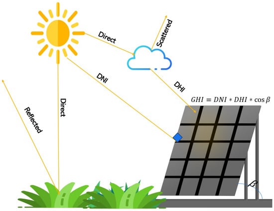
Figure 1.
GHI components and solar PV interception.
A key strength of this work lies in the adaptability of the proposed solution across six distinct solar forecasting sites. This versatility is attributed to the extensive preprocessing and analysis steps, which leverage multiple time-shifted versions of GHI values along with their relevant linked features. The application of autocorrelation and partial autocorrelation analyses facilitates the identification of optimal time shifts, ensuring the best possible performance from the regressors. This was validated through an in-depth analysis of metric variations across different shift configurations. Furthermore, the study highlights the varying responses of different ensemble compositions across sites, with models consistently achieving high values. The integration of explainable AI (XAI) techniques further enhances interpretability, allowing for a comprehensive investigation and validation of results by identifying the most critical features. In terms of generalization, the proposed approach outperforms those in the existing literature by effectively addressing previously overlooked challenges, thereby advancing the state of the art in solar forecasting.
Table 2.
Summary of solar irradiance forecasting studies.
Table 2.
Summary of solar irradiance forecasting studies.
| Reference | Contribution | Models Used | Result |
|---|---|---|---|
| [17] | Develop a real-time solar irradiance forecasting technique | Cloud tracking techniques, implanted fisheye network camera, ANN algorithm | The techniques outperformed existing forecasting models at two locations. |
| [18] | Review the use of ANNs in solar power generation forecasting and analyze measurement instruments | ANN | ANN usage increases accuracy; hybrid systems and instrument calibration improve accuracy. |
| [19] | Forecast hourly GHI using ensemble model | Extreme gradient boosting forest, deep neural network, ridge regression | The proposed model outperformed standalone ML and DL models in stability and accuracy. |
| [20] | Compare ML and DL methods for predicting solar irradiance | SVR, Random Forest, polynomial regression, ANN, CNN, RNN | DL algorithms were more accurate but required more computational power than ML algorithms. |
| [21] | Predict daily solar irradiance | Feed Forward Neural Nets (FFNNs), empirical models, Holt–Winters, RSM | ANN model outperformed Holt–Winters, RSM, and empirical models. |
| [22] | Model solar radiation using robust soft computing method | Least square support vector machine, multi-verse optimizer algorithm, genetic algorithm, gray wolf optimization, sine cosine algorithms | The proposed technique outperformed others in terms of accuracy. |
| [23] | Develop hourly day-ahead solar irradiance forecasting model | LSTM+RNN, FFNN | The proposed approach outperformed FFNN; simulation showed 2% increase in annual energy savings. |
| [24] | Predict solar irradiance using hybrid models and probabilistic forecasts | PSO-XGBoost, PSO-LSTM, PSO-GBRT, ANN, CNN, LSTM, RF, GBRT, XGBoost | PSO-LSTM showed superiority for day-ahead solar prediction. |
| Current | Predict GHI for the next temporal step with 6 different stations at once, different characteristics, and different lagged versions | Tree-based algorithms, MLP, ensemble learners | Tested with different sites that have different features. Analyzed the impact of GHI for different time-shifted input data. |
1.2. Motivation, Contributions, and Organization
Predicting solar irradiance is crucial for optimizing solar power generation, ensuring grid stability, and supporting energy forecasting and trading. Accurate irradiance forecasts enhance climate and weather modeling, aiding in climate research and agricultural planning. They also play a vital role in environmental monitoring, air quality management, and assessing renewable resources. Moreover, reliable solar irradiance predictions inform energy policies, investment decisions, and the development of advanced solar technologies. Leveraging machine learning for this purpose promises improved accuracy and efficiency, thereby maximizing the benefits of solar energy and contributing to a sustainable future.
In this work, we enhance our latest solar irradiance prediction scheme, developed in [4], in terms of generalization. We use several stations of PV panels and create time-lagged versions of the data, meaning that a new dataset is generated by considering windows of historical feature values and forecasting the next GHI value and time , where is a step into the future. Our approach involves analyzing data from multiple solar panel sites in diverse locations. This allows us to provide a detailed analysis of the features that improve prediction accuracy for each site. Subsequently, we establish a consensus on the most critical features for a generalized machine learning model. This model aims to predict solar irradiance effectively across different sites with similar configurations. Our methodology represents a novel approach as it transitions from localized prediction models to a more generalizable framework. The results of this study could surpass the limitations of site-specific models, offering a versatile solution for solar irradiance prediction.
The remainder of the paper is structured as follows. Section 2.1 details the dataset, the designed framework, the machine learning models utilized, the evaluation strategies adopted, and the steps taken for exploratory data analysis. Section 3 presents findings from six stations, evaluating the performance of various machine learning models across different time shifts and forecasting horizons. This section also employs explainable AI (XAI) techniques to interpret the results, offering valuable insights into model behavior and the significance of features. Lastly, Section 4 summarizes the key findings, highlights the study’s contributions, and identifies promising directions for future research and practical implementations.
2. Proposed Solution
This section details the complete operational pipeline of the proposed solar irradiance forecasting solution. We address all steps, with a focus on reproducibility, from data acquisition and cleaning to model training and evaluation. The core goal is to enable reproducibility across all stations using a unified and explainable machine learning framework. The developed solution incorporates a generalizable approach that utilizes data from various PV stations located in different regions, each with distinct characteristics, encompassing DNI, DHI, and GHI, which are the targets of the prediction. However, the prediction is not solely based on raw data. As the analysis will demonstrate, there is a strong correlation between the current GHI value and its lagged versions. Therefore, a windowing function is created to generate data based on these windows, enabling the forecasting of future values based on past observations.
2.1. Dataset Presentation and Acquisition
The Measurement and Instrumentation Data Center (MIDC) dataset provides comprehensive data from various solar radiation measurement stations. The dataset includes both active and inactive sites, and users can access the data via a raw data API. This API facilitates automated extraction of daily datasets from any MIDC station, ensuring that users receive data equivalent to that retrieved using the “All Raw Data” option from the MIDC daily data web interface [25]. The key features of the dataset are as follows:
- Station identifier: Each station is uniquely identified by an 8-character code.
- Date range: Users can specify a date range (begin and end dates) for data extraction with the format YYYYMMDD. If no dates are specified, the most recent day’s data is returned by default.
- Comprehensive headers: Each dataset includes a header describing the columns, which may change over time. Users should read the header for proper usage.
- Instrument configuration changes: If the specified date range spans an instrument configuration change, the API returns an error, indicating the date of the change. Users need to make separate queries for data before and after the change.
- Field API: Before querying the Data API, users can call the Field API to know the available measurement parameters for a station over time.
- Station List API: Provides a comma-separated list of station identifiers, names, latitude, longitude, and elevation.
- AIM Meta Data API: Offers information on instrument calibration history, location, maintenance, etc.
A set of these station descriptors and their sites is presented in Table 3. In this work, six stations were selected, and for each one, data spanning three years were downloaded using the MIDC Raw Data API with the “All Raw Data” configuration. The download script filtered for the following:
Table 3.
A set of possible station IDs and names.
- Station ID and name.
- Date range between January 2020 and December 2022.
- All available environmental and irradiance parameters (e.g., GHI, DHI, DNI, temperature, pressure).
Each station’s raw file was converted to a pandas DataFrame with unified timestamp formatting in 30 min intervals. Files were synchronized by their UTC timestamps, and any misaligned rows were dropped to ensure uniformity across features and stations.
2.2. Proposed Framework
The data processing and modeling workflow for multi-site solar irradiance prediction is illustrated in Figure 2. It integrates a unified preprocessing pipeline, time-lagged feature engineering, and model training strategy across diverse PV stations. Below is the detailed sequence of steps:
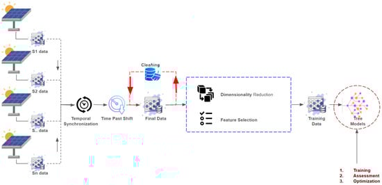
Figure 2.
The proposed framework for GHI prediction.
- Data collection from multiple PV sites: Solar irradiance and environmental data were collected for six PV stations over three years using the MIDC Raw Data API. For each site, the raw files were parsed into structured DataFrames with consistent timestamp formatting (30 min resolution).
- Data preprocessing pipeline: The preprocessing consisted of the following clearly defined steps:
- –
- Synchronization and alignment: All station data were synchronized based on UTC timestamps. Any mismatched timestamps or duplicated entries were dropped. Feature names were standardized (e.g., GHI, DHI, DNI) across stations to ensure schema consistency. This means that columns were renamed and standardized (e.g., “Global Horizontal” → “GHI”). Units were converted where necessary to ensure consistent W/m2 scales.
- –
- Concatenation: After alignment, datasets from the six stations were concatenated into a unified dataset. Each row retained its station identifier, enabling station-specific modeling and evaluation while allowing for global analysis.
- –
- Data cleaning:
- ∗
- Features with more than 30% missing values were dropped.
- ∗
- Remaining missing values were imputed using forward-fill interpolation.
- ∗
- Outliers were identified using the IQR method and removed per feature.
- –
- Resampling and time lagging: Each DataFrame was resampled to a specific interval. Then, a windowing function was applied to generate time-lagged features. Specifically, lagged versions of GHI, DHI, DNI, and other relevant features were created for , , …, intervals (e.g., past 30, 60, 90 min) to support prediction at or .
- Feature selection: A two-step feature selection strategy was adopted:
- –
- Kendall correlation coefficients were calculated between all feature pairs, excluding the target variable. To mitigate multicollinearity, one feature from each highly correlated pair (correlation coefficient > 0.95) was removed. Furthermore, Kendall correlation coefficients were also computed between each feature and the target variable (GHI). Features exhibiting a correlation coefficient below 0.3 with the target were discarded. This selection process ensured the retention of the most relevant and informative predictors.
- –
- Feature importance scores were computed using an ensemble of tree-based models. The importance scores were averaged across models, and the top 15 most influential features were retained for each station.
- –
- Incremental feature selection: To further refine the input space and evaluate the contribution of individual features, an incremental feature selection strategy was applied. Starting from the most important feature, models were iteratively trained by progressively adding one feature at a time. At each step, model performance was evaluated using validation metrics (e.g., RMSE and R2). This approach enabled the identification of the optimal subset of features that maximized predictive performance while minimizing the risk of redundancy and overfitting.
- Model training and evaluation strategy:
- –
- Training pipeline: The predictive task is formulated as a regression problem. The following steps were performed for each station independently:
- ∗
- Train/test split: Each station’s cleaned and feature-selected dataset was split into 80% training and 20% testing sets. To avoid data leakage and ensure temporal integrity, the dataset for each site was chronologically ordered. We then used a single-split strategy, where the first 80% of the observations (based on timestamps) were used for training and the remaining 20% were reserved for testing. This approach avoids shuffling or interleaving of future observations into the training set.
- ∗
- Model initialization: Each model was initialized using a fixed random seed (42) to ensure reproducibility.
- ∗
- Multiple regressors were trained: MLPRegressor (3 × 100 hidden layers), GradientBoosting, RandomForest, CatBoost, ExtraTrees, etc. All models used fixed seeds and default hyperparameters for reproducibility. The set of employed models includes:
- ·
- MLPRegressor: The best configuration for the model was with 3 hidden layers, each with 100 neurons, relu activation, Adam optimizer, and 10,000 epochs.
- ·
- GradientBoosting, RandomForest, ExtraTrees, CatBoost, XGBoost, LightGBM: All tree-based regressor models were initialized using Scikit-learn default parameters, with hyperparameter tuning skipped for uniform comparison.
- –
- Model evaluation: Each model’s performance was evaluated using five metrics: R2, RMSE, MAE, median absolute error, and MAPE.
- Ensemble modeling: In addition to standalone models, to improve generalization, a stacking-based ensemble was built for each station. Stacking ensemble models were implemented using Scikit-learn’s StackingRegressor with 5-fold internal cross-validation.
2.3. Description of ML Models and Performance Metrics
In this work, machine learning was employed to predict solar irradiance, addressing a regression task aimed at forecasting a continuous variable. In line with this framework, tree-based and ensemble learning models were utilized [26,27,28]. A description of the models used, which are initialized with a random state of 42 to ensure reproducibility, is provided below.
- MLP: A Multi-Layer Perceptron regressor with a neural network architecture consisting of three hidden layers, each containing 100 neurons. The model is set to run for a maximum of 10,000 iterations.
- Decision TreeRegressor: A decision tree regressor that uses a tree-like model of decisions to predict a target value.
- RandomForest: An ensemble learning method that constructs a multitude of decision trees during training and outputs the mean prediction of the individual trees.
- ExtraTrees: An ensemble learning technique similar to the RandomForest, but it uses the entire dataset instead of a bootstrap sample and selects split points at random.
- GradientBoosting: An ensemble technique that builds trees sequentially, each one correcting errors made by the previous ones.
- CatBoost: A gradient boosting regressor that handles categorical features natively and is designed to be fast and accurate. The model has its verbosity set to 0 to suppress output during training.
- LightGBM: A gradient boosting framework that uses tree-based learning algorithms. It is designed to be efficient and fast, especially with large datasets.
- XGBoost: An optimized distributed gradient boosting library designed to be highly efficient, flexible, and portable.
While and RMSE metrics are commonly used in regression tasks, and MAE to some extent, other metrics can also be significant. The performance metrics used in this work are depicted in Table 4.
Table 4.
Regression metrics.
2.4. Exploratory Data Analysis
The distributed data is characterized by unique features at each site. However, to predict the GHI for the next time step, the GHI values must be present in the dataset. This requirement is met by the stations considered. For instance, the features of 3 different stations, Natural Energy Laboratory of Hawaii Authority (NELHA), University of Louisiana at Lafayette (ULL), and Cal Poly Humboldt SoRMS (HSU), are described in Table 5. Two more stations were used in the training, namely, REL Flatirons Campus (NWTC) and the University of Florida (UFL).
Table 5.
Environmental data descriptions and units for three stations.
The exploration of these features toward the development of an optimal solution was performed based on the queries described below.
- What does the outlier study reveal?Outlier analysis, an essential step for detecting factors such as fluctuations in incident radiation, solar panel performance, and faults, was performed at the three sites. The presence of outliers can be attributed to various factors beyond those initially mentioned. Notably, outliers were observed in the GHI series across all stations, as shown in Figure 3. At the NELHA site, outliers were found in the global PAR, global UV-PFD, and global UV measurements. At the HSU site, outliers were present in the diffuse irradiance variants, direct normal irradiance, and to some extent, the airmass feature. Lastly, at the ULL station, outliers were detected in the GHI, DNI, DHI, and CR1000 temperature measurements. Outliers in solar irradiance data often result from rapid and unpredictable changes in environmental conditions, sensor inaccuracies, and calibration issues. For instance, GHI outliers across all stations may stem from sudden weather changes, such as cloud cover or precipitation, which impact the total solar radiation measured. At the NELHA site, outliers in global PAR, UV-PFD, and UV measurements could be due to local variations in vegetation or atmospheric conditions. At the HSU site, the presence of outliers in diffuse irradiance, direct normal irradiance, and the airmass feature suggests sensitivity to atmospheric variability and measurement inconsistencies. Finally, the ULL station exhibited outliers in GHI, DNI, DHI, and CR1000 temperature readings, likely caused by sudden temperature fluctuations or sensor exposure to environmental factors. Understanding these causes is crucial for improving data accuracy and the reliability of solar irradiance forecasts. The UNLV station, in contrast, exhibited outliers in only two series: GHI and wind cloud temperature. This suggests the impact of these values on the model’s performance in relation to the time-shifted values. Similar to the UNLV station, the RAZON station had outliers present in only two series, GHI and DNI, whereas the NWTC station was characterized by the absence of outliers.
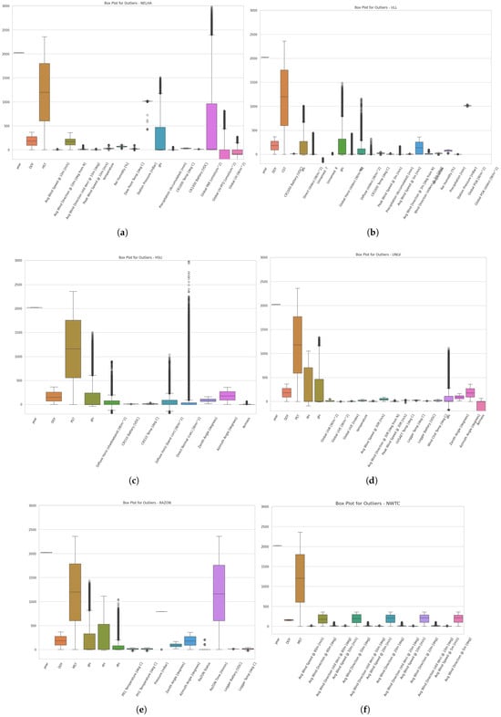 Figure 3. Outlier analysis for (a) NELHA, (b) ULL, (c) HSU, (d) UNLV, (e) RAZON, and (f) NWTC.
 - What does the correlation study reveal?Correlation analysis was conducted in parallel across all station features using the Kendall method due to its robustness against outliers, as shown in Figure 4. This analysis highlighted variability in feature correlations across different sites. For example, the features most correlated with the GHI series were global PAR, CR1000 temperature, solar PV temperature, and average wind direction, with all but wind direction showing correlations exceeding 50%. At the ULL station, the GHI series was highly correlated with DNI and DHI, with the CR1000 temperature and solar panel temperature also being notable factors, although solar panel temperature had a correlation of 50%. At the HSU station, the CR510 battery and temperature showed the strongest correlations with the GHI. From these observations, it can be inferred that the CR1000 temperature, components of the GHI, and solar panel temperature are key factors in predicting GHI across stations. These features exhibit positive correlations with the GHI. Conversely, negative correlations were noted for relative humidity, CR1000 battery, and zenith angle, suggesting these factors may inversely affect GHI predictions. The NELHA station is characterized by a high correlation between the global PAR and GHI, as well as the CR1000 and temperature measurements. The UNLV station exhibits the best feature correlations and is similarly characterized by values of GHI that are correlated with global UVA, UVB, and the components of GHI, which are DNI and DHI. Additionally, the airmass shows a good correlation with the target. For the RAZON station, the components of GHI, PR1, and PH1 temperatures, pressure, and the RAZON status with the azimuth angle all demonstrate a correlation with the target that exceeds 50%. It is also important to note the presence of negative correlations. For some stations, the zenith angle can have a positive correlation with the target, while for others, it may have a negative impact. This can also be extended to the azimuth angle. Furthermore, features with a correlation of less than 0.3 can be dropped, which is a threshold used particularly for stations that have strong correlations, exceeding 50%, with the target GHI.
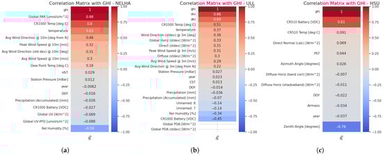
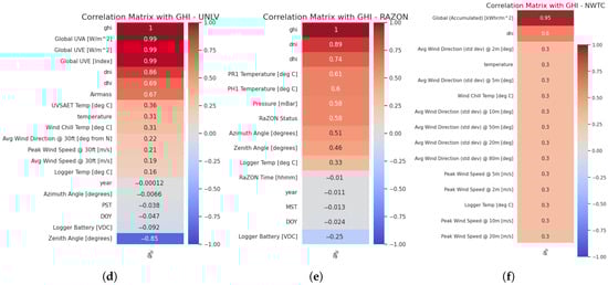 Figure 4. Correlation analysis for the different stations with GHI: (a) NELHA, (b) ULL, (c) HSU, (d) UNLV, (e) RAZON, and (f) NWTC.
 - How is GHI linked to the time-lagged versions?In this step, we focused on the lagged version of the GHI across the three stations ULL, NELHA, and HSU. We performed autocorrelation and partial autocorrelation analyses using the ACF and PACF functions over a 30-min horizon. This involved resampling the data to 30 min intervals and examining how the GHI values are related to past values at intervals of 30 min, 1 h, and 1.5 h. We considered the NELHA station as an example for the tests. The results of these analyses are shown in Figure 5.
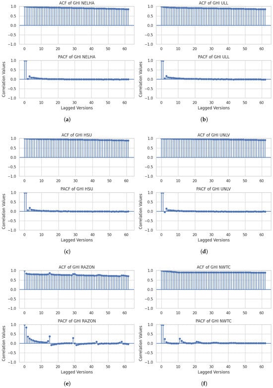 Figure 5. ACF and PACF for (a) NELHA, (b) ULL, (c) HSU, (d) UNLV, (e) RAZON, and (f) NWTC.For the NELHA station, the time-lagged versions exhibit degrading behavior over time. The PACF, on the other hand, indicates that the current GHI value is primarily linked to two highly correlated past values. Additionally, smaller correlation values extend up to five past values, which correspond to a time lag of up to 3 h. A similar observation is noted for the ULL and HSU stations, where these lagged versions of GHI are mainly correlated with the values from the last 30 min. This raises another question about how many historical shifts can influence the final results. As detailed in the previous analysis, a notable relationship exists between the shifted and current values of GHI. This relationship is particularly significant when constructing data windows for prediction models. Three main machine learning models—RandomForest (RF), CatBoost, and Multi-Layer Perceptron (MLP)—were employed to analyze the impact of these shifted values on GHI prediction. The selection of these models was based on their demonstrated efficacy in previous research on GHI prediction [4]. A thorough analysis was conducted for at least eight past shifts, with the results illustrated in Figure 6 and Figure 7 for 30 min-ahead, 1 h-ahead, and 2 h-ahead forecasting. The analysis of the shift influence on the variations in and RMSE was performed for all the stations across 8 shifts. For , it can be observed that for a 30 min shift, all stations exhibit a consistent result across the 8 shifts, except NWTC and, to some extent, the ULL station. However, when using shifts with higher time intervals, such as 1 h and 2 h, the results become unstable, except for the UNLV station, which shows stable performance. This could indicate that, regardless of the shift considered, the UNLV station’s model performance will remain stable. For RMSE, stable performance is observed for a 30 min shift, except for the NWTC station. For 1 h and 2 h shifts, across the 8 shifted values, a non-stable performance is observed for all stations, with minimal instability for the UNLV station. It can be concluded that the shift changes impact the and RMSE performance values for all stations, except for the UNLV station, where the change is minimal yet exists.
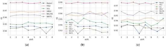 Figure 6. Shift impact on for different forecasting horizons: (a) 30 min, (b) 1 h, and (c) 2 h.
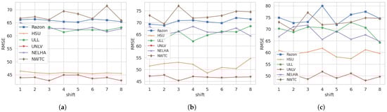 Figure 7. Shift impact on for different forecasting horizons: (a) 30 min, (b) 1 h, and (c) 2 h.
 - Which features hold significant impact as predictors?In alignment with the previous procedure, a tree average importance technique was applied to the three stations NELHA, HSU, and ULL to identify the optimal features that lead to the best outcomes within the regressors. For the NELHA site, when considering only the 10 most important features, it was found that the lagged version of GHI up to 30 min (from GHI at T-1 to GHI at T-30 min), the accumulated global irradiance up to a 30 min lag, and up to three lags were the most impactful features for predicting GHI at T+30 min. Other significant factors included two lagged versions of the accumulated irradiance and three-to-five lagged versions of GHI. For the ULL site, the important features were limited to the lagged version of GHI up to 30 min in the past, and to a lesser extent, the second lagged versions up to 1 h earlier. Other values were mostly not significant. This pattern extended to the HSU site, where only two features were crucial: the lagged version of GHI up to 30 min and the lagged version of the zenith angle up to 30 min. These observations indicate a common consensus across all sites, highlighting that the most important feature for prediction is the first lagged version of GHI. All these results can be seen in Figure 8.
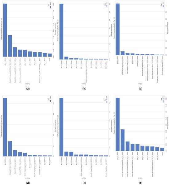 Figure 8. Feature importance for the different stations: (a) NELHA, (b) ULL, (c) HSU, (d) UNLV, (e) RAZON, and (f) NWTC.
3. Results and Discussion
The dataset was obtained from six different stations. After applying preprocessing steps and conducting exploratory data analysis, we gained insights into impactful features and existing correlations. This analysis also identified possible historical steps (time steps) that could be used to obtain the most accurate GHI values. The dataset was then passed to a windowing function, allowing the use of the current and historical 30 min of data to predict the next 30 min of GHI. Training and testing sets were created in a ratio of 80% to 20%, respectively. The full training was performed in Google Colab, a free Python (version 3.11.13) development and data analysis framework provided by Google. Scikit-learn was primarily used for loading the ML models [26], except for the MLP, which utilized the Keras and TensorFlow libraries. Primarily, tree-based algorithms were utilized, and ensemble learners were created using different tree-based frameworks and a simple MLP architecture. This approach aimed to provide a lightweight solution that could be generalized to various sites simultaneously. The composition of the ensembles and the individual learners is detailed in the aforementioned sections. The results, considering the 30 min-lagged version of the features and results as references, are provided below in the following order:
- −
- Results from each station: NELHA, ULL, HSU, UNLV, NWTC, and RAZON;
- −
- Ensemble learners in different stations;
- −
- Hourly GHI prediction and link with time-lagged versions;
- −
- Sensitivity analysis through time shifting;
- −
- UNLV use case.
3.1. Results from Each Station
For each station, tree-based algorithms and ensemble learners were trained for the prediction of GHI, and then a thorough analysis of the importance of the characteristics considered by the top-performing model was conducted. Different combinations of standalone models were used in an ensemble framework and tested to gain insight into the collaborative performance and the possibility that it surpasses standalone models.
- NELHA: This station is characterized by the presence of 19 features, of which several were found to be correlated with the target variable, as shown earlier. Moreover, a study was conducted on the correlations that can be found between features with the consideration of the past time shift. This is visualized in the correlation heatmap in Figure 9a. The correlations exceed 90% for the shifted GHI values with the global PAR. In addition, the shifted HST values also demonstrate strong correlations, reaching 88%. This indicates that a possible construction of a feature model could enclose these shifted values. The results from the models trained on this station are depicted in Table 6. It can be seen that the best results are obtained when using the GradientBoosting regressor, achieving an of 0.96 and an RMSE of 63.61, followed by the MLP and the RandomForest regressor. Overall, all the models performed well, except the decision tree. As for the residual analysis at the NELHA station in Figure 10a, it indicates that the errors are centered around 0, predominantly ranging between −200 and 200. However, errors can occasionally reach values between −400 and 400. Points outside these intervals suggest the presence of outliers or potential overfitting of the model.
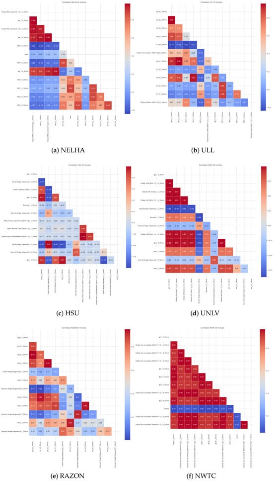 Figure 9. Time-shifted correlated features for (a) NELHA, (b) ULL, (c) HSU, (d) UNLV, (e) RAZON, and (f) NWTC.
Table 6. Model performance comparison across different stations.
Figure 9. Time-shifted correlated features for (a) NELHA, (b) ULL, (c) HSU, (d) UNLV, (e) RAZON, and (f) NWTC.
Table 6. Model performance comparison across different stations.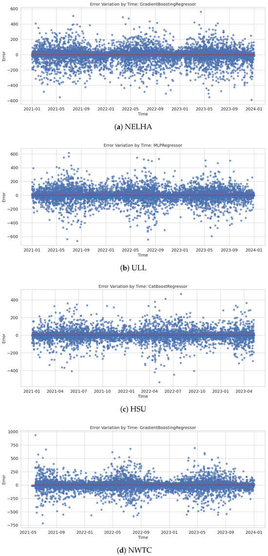 Figure 10. Residual analysis for the different stations: (a) NELHA, (b) ULL, (c) HSU, and (d) NWTC.
 - ULL: The correlation heatmap in Figure 9b and performance table in Table 6 provide a comprehensive view of the relationships between various time-shifted irradiance measurements and their impacts on model performance. The high correlation between ghi_t1_30min and ghi_t2_30min at 0.96 indicates a strong temporal autocorrelation, which is also reflected in the significant correlation of 0.91 with other features such as dni_t1_30min (0.86) and ghi_t3_30min. This suggests that GHI measurements are closely related to direct normal irradiance (DNI) over short time intervals. Furthermore, the moderate correlation between dni_t1_30min and dhi_t1_30min at 0.70 highlights the partial dependency between direct and diffuse horizontal irradiance (DHI). The models’ performance metrics, with values ranging from 0.89 to 0.95, demonstrate that models like the MLPRegressor and CatBoostRegressor can capture these intricate relationships effectively. The low RMSE and MAE values further underscore the models’ accuracy in predicting irradiance values, with MLPRegressor showing the best overall performance. This indicates that leveraging these correlations can significantly enhance predictive modeling in solar irradiance forecasting. Residual analysis at the ULL station in Figure 10b demonstrates a generally good performance by the MLP regressor. The errors are centered around 0, with most falling within the range [−200, 200]. However, some data points exhibit errors reaching up to 600.
- HSU: In this case, 12 features were considered, with those directly associated with GHI—namely, DNI, DHI, and GHI itself—being excluded. The remaining 12 features were retained due to their high correlation with the target variable, as presented in Figure 9c. The correlation heatmap observations highlight significant relationships among various features over 30 min intervals. Notably, the correlation between ghi_t1_30min and ghi_t2_30min is high at 0.97, indicating strong temporal autocorrelation in GHI measurements. Moreover, ghi_t1_30min shows strong correlations with CR510 Battery [VDC]_t1_30min0.82 and ghi_t3_30min at 0.92, suggesting consistent patterns in GHI over time. Zenith Angle [degrees]_t1_30min has a strong negative correlation with ghi_t1_30min at and ghi_t2_30min at , indicating that as the sun ascends, the GHI increases. Furthermore, Azimuth Angle [degrees]_t6_30min shows moderate correlations with other features, like Zenith Angle [degrees]_t1_30min at 0.47 and Zenith Angle [degrees]_t-2_30min at 0.99, reflecting the sun’s position and its impact on irradiance. Lastly, the high correlation at 0.89 between Direct Normal (calc) [W/m2]_t1_30min and Diffuse Horiz (shadowband) [W/m2]_t1_30min indicates a strong relationship between these two types of irradiance. On the other hand, the model performance table in Table 6 highlights that CatBoostRegressor and other ensemble methods like GradientBoostingRegressor and RandomForestRegressor achieve high values (approximately 0.97), indicating strong predictive capabilities. These models also exhibit low RMSE and MAE values, confirming their accuracy in predicting irradiance values. The median absolute error (median AE) is consistently low, particularly for RandomForestRegressor and ExtraTreesRegressor, suggesting fewer large prediction errors. When visualizing Figure 10c, the CatBoost regressor residuals analysis for predicting GHI in the next 30 min across the time axis, it is evident that the errors are generally within ±200. Only a few outliers exceed this range, indicating that the model performs well over the entire three-year dataset. It can also be observed that this error margin narrows to less than ±100 at certain time points, such as between January 2022 and March 2022.
- UNLV: A total of 20 features exist at this station, representing the GHI variations, the ambient conditions, and the performance monitoring of the solar panels. The time-shifted values revealed a strong correlation between global UVA and UVE for up to 2 h, as depicted in Figure 9d. Similarly, shifted GHI and DNI values showed high correlation for up to 1 h. Subsequently, tree-based algorithms were trained to predict GHI values for the next 30 min. The performance comparison of the models shows that all tested algorithms achieve high values, indicating strong predictive accuracy, as viewed in Table 6. RF performs slightly better, with the highest of 0.9814 and the lowest MAE of 14.67, reflecting minimal average prediction error. CatBoostRegressor follows closely, with similar accuracy but a slightly higher RMSE and MAE. MLPRegressor and GradientBoostingRegressor show good performance as well, though they exhibit higher RMSE and MAE compared to RF. ET is comparable to RF in terms of and error metrics. DecisionTreeRegressor, while having a lower and higher RMSE and MAE, still shows reasonable performance but with less accuracy. In this comparison, RandomForestRegressor emerges as the most effective model.
- RAZON: The RAZON station is characterized by 15 features that include the GHI, DNI, DHI, ambient conditions, solar PV temperature, azimuth angle, and battery operating conditions. The training process, like all the other stations, consisted of studying the correlation with lagged versions and employing the most influential features as inputs for the models. Figure 9e provides a feature correlation study, while Table 6 provides the obtained results. The correlation heatmap for RAZON over 30 min intervals reveals significant relationships among the variables, particularly between the GHI and DNI across different time shifts (, , , …). Notably, the GHI values at and have very high positive correlations with each other, at 0.95, and with DNI at corresponding time shifts. Conversely, the azimuth and zenith angles exhibit lower correlations with irradiance variables, indicating less dependency. This suggests that while the angles provide important contextual data, the irradiance measures are more interdependent. This analysis underscores the critical role of temporal shifts in understanding irradiance patterns and their predictive modeling. The performance analysis in Table 6 reveals that the GradientBoostingRegressor and RandomForestRegressor models exhibit the highest values (0.8903 and 0.8897, respectively), indicating strong predictive accuracy. RandomForestRegressor slightly outperforms the other models in terms of MAE, with a value of 28.47 compared to GradientBoostingRegressor’s 30.93, suggesting it has lower average prediction errors. ExtraTreesRegressor shows similar performance to RandomForestRegressor but with slightly higher RMSE and MAE. MLPRegressor has a significantly higher MAE (56.59) and RMSE (108.05), indicating poorer performance. CatBoostRegressor also performs well, though not as effectively as GradientBoosting or RandomForest, with an of 0.8650 and higher RMSE and MAE. DecisionTreeRegressor shows the lowest performance, with the lowest of 0.8238 and the highest RMSE of 131.79, indicating higher prediction errors and less accuracy compared to the other models. In this comparison, RandomForestRegressor and GradientBoostingRegressor are the most effective models.
- NWTC: The NWTC station is characterized by the presence of more than 20 features, from the ambient to the operating conditions and the GHI, DHI, and DNI values. In this station, as shown in Figure 9f, all features exhibit a strong correlation with values shifted by 30 min, except for the monthly series, which displays weak correlations. This is expected, given that the PACF and ACF functions are designed to capture dependencies in lagged values up to 30 min. The model’s performance, shown in Table 6, reveals that GradientBoosting stands out, with the highest value of 0.9942, demonstrating superior predictive accuracy and the best fit to the data. It also has the lowest RMSE of 71.26 and a low MAE of 34.00, indicating minimal average prediction errors and superior precision. In contrast, the MLP, with the lowest of 0.9744 and the highest RMSE of 149.92, shows the weakest performance, reflecting higher prediction errors and less accuracy. RandomForest and CatBoost also perform well, with high values of 0.9893 and 0.9868, respectively, and relatively low error metrics, though slightly less favorable than GradientBoosting. Notably, ExtraTrees exhibits higher errors compared to these top models, while DecisionTree, though strong, has a slightly higher RMSE and MAE than the top performers. Residual analysis at the NWTC station in Figure 10d demonstrates generally good performance by the GradientBoosting regressor. The errors are centered around 0, with most falling within the range [−250, 25]. However, some data points exhibit errors reaching up to 982.
It is important to highlight that for the training set consisting of 10,000 samples, selected to maintain a balanced trade-off between model performance and computational complexity, the standalone regressors (including RandomForest, XGBoost, CatBoost, and MLP) required on average approximately 0.6 s to complete training. This corresponds to roughly seconds per sample, illustrating the high efficiency of these models in both the training and inference phases. Moreover, the models demonstrated rapid convergence on the testing set due to the adopted feature engineering strategy. In particular, when using only lagged GHI features, specifically the current and one-prior time step, the decision-making process becomes significantly simplified. This reduction in input dimensionality enables the models to focus on the most temporally relevant information, minimizing redundancy while preserving forecasting accuracy. This simplicity has substantial implications for deployment in resource-constrained environments, such as IoT-based edge devices used in smart grid applications. The lightweight nature of the trained models, both in terms of size and computational requirements, facilitates fast inference with minimal memory and processing demands.
3.2. Ensemble Learners in Different Stations
Training ensemble learners is a key factor in many classes of problems in machine learning, especially those related to the energy domain, as proven in [29]. Thus, a particular step was taken to combine the best learners in the first step of training to explore the possibility of building a powerful ensemble model that can be used across all stations. Table 7 depicts the obtained best combination in each station. Several combinations of tree-based models were tested using the Optuna framework (Appendix A), aiming to develop a robust model that can be generalized across all stations. Despite these efforts, it was observed that the best results for each station did not surpass those obtained with single models, as presented in Table 7 and Figure 11. However, what is particularly intriguing is the superiority of the stacking ensemble over other ensemble techniques, such as voting and bagging, across all stations, even when the composing learners differed. This finding suggests that a potential general model could benefit significantly from the stacking technique. Furthermore, it was observed that, for all stations, the GradientBoosting framework was essential for the composition of the models. Typically, this framework could be complemented with an MLP or a RandomForest model. This suggests that a stacking-based general model could leverage the strengths of these models, combined with other powerful techniques, to achieve optimal performance. The power of stacking lies in its ability to combine the predictions of multiple models, thereby improving accuracy and robustness. This ensemble method outperformed others by effectively capturing the strengths of its individual learners, indicating its potential to create a generalized high-performance model applicable to various stations. This assumption forced the expansion of the obtained results shown in Table 7 for a 30-min shift to verify the performance under a 1-h shift. As expected, resampling the data from 30-min intervals to hourly intervals led to a reduction in the number of samples. To compensate for this shrinkage and ensure statistical robustness, data augmentation was performed using PVLib to acquire additional samples. A total of 20,000 samples was used at this stage. All stations were retrained using a hybrid model combining the GradientBoosting and RandomForest algorithms. The results in Figure 12 demonstrate that, despite the coarser temporal resolution, the stacking model maintained strong performance across stations. The UNLV station achieved the best accuracy, with an of 0.997 and an RMSE of 10.13, while the RAZON station showed relatively lower performance, with an RMSE of 98.29 and an of 0.910. This variation suggests that, while the proposed model generalizes well, station-specific dynamics still influence performance, warranting further exploration of localized tuning or model adaptation strategies.
Table 7.
Results for different stations using a 30-min shift.
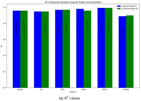
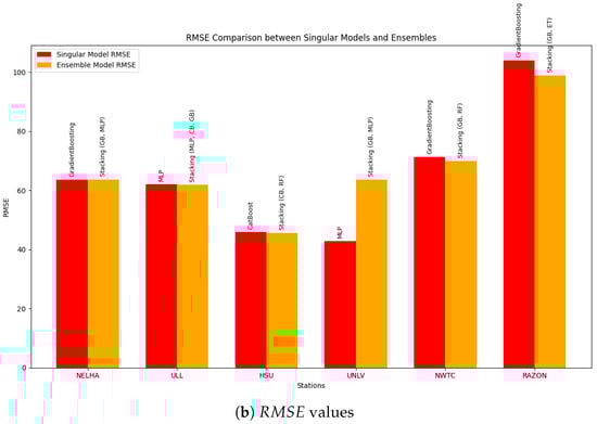
Figure 11.
Comparison between single models and ensemble in terms of (a) and (b) RMSE.
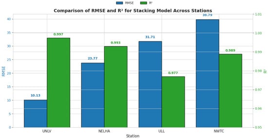
Figure 12.
Results from ensemble learning on all stations for 1-h shift.
In this step, confidence intervals (CIs) are calculated to evaluate the performance of the stacking-based ensemble model for predicting GHI in four different stations, incorporating bootstrap-based uncertainty estimates. The model’s predicted mean aligns closely with the actual measurements, indicating strong predictive accuracy. A 95% confidence interval, standard in uncertainty quantification, captures the variability across bootstrap replicates. This interval remains narrow in most cases, reflecting high model confidence, but widens during periods of low solar radiation, indicating increased uncertainty. The visualization in Figure 13 clearly conveys both the accuracy and uncertainty of the forecasts, which is essential for risk-sensitive applications such as solar energy management. This performance, demonstrated at the UNLV station, can be confidently generalized to the NELHA station. At the ULL and NWTC stations, the model exhibits a marked improvement over earlier versions, achieving a much closer alignment between predicted and actual values. The updated plot features tighter, more consistent confidence intervals and captures fluctuations more effectively, suggesting enhanced robustness and generalization, likely due to refined bootstrapping and model calibration techniques.
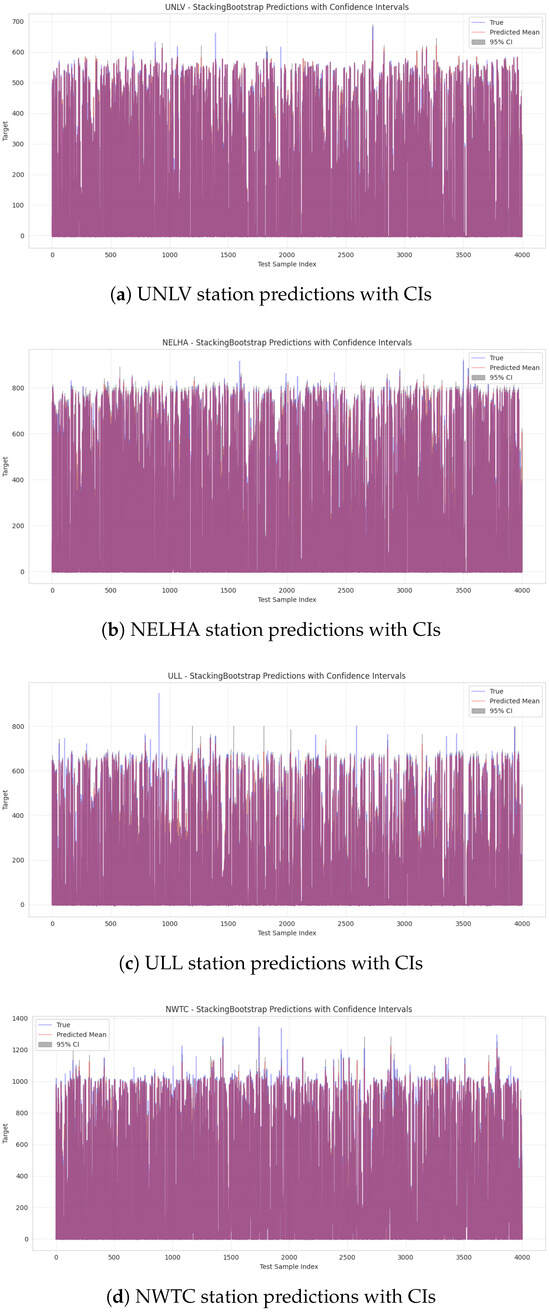
Figure 13.
Analysis of stacking ensembles on 4 different stations with confidence intervals.
3.3. Hourly GHI Prediction and Link with Time-Lagged Versions
In the third step, we examined how model performance varied across all stations when using different time-shifting windows. The analysis was mainly extended to 1-h shifting and forecasting. Table 8 comprehensively compares all metrics for the 30 min- and 1 h-lagged temporal shifts. It is observed that extending the forecasting and shifting horizons results in a deterioration in the model’s performance at the NELHA station, particularly evident in the RMSE metrics. The best-performing model also changed to the MLP. Similar observations were made for the NWTC station, where the ExtraTrees model proved to be the best performer. However, for other stations, the models performed well for both forecasting horizons. This indicates that the models effectively account for the impact of the shift and the forecasting horizon due to the efficient feature selection technique, which includes the shifted versions of the GHI. One possible reason for performance degradation over varying time shifts, especially with increased data versions, is the reduction in the number of samples in the dataset, particularly when starting with a lower sampling rate. This limitation means that models have less data to analyze. It is also noteworthy that for the 30-min shift, the MLP was the best-performing model at two different stations. For the 1-h shift, it was selected as the best performer at three stations. This pattern aligns with the fact that neural networks, including MLPs, are powerful deep learning models, particularly effective for mid-to-long-term forecasting horizons, making this level of performance expected.
Table 8.
Model performance comparison for 30-min and 1-h shifts.
The stability of model performance across the majority of stations for the 1-h lagged version of GHI was confirmed through an analysis of hourly GHI values at t, , and for all stations, as depicted in Figure 14. The projection revealed a general correlation between these GHI values, as evidenced by the dense diagonal distribution observed in all stations. For example, the RAZON station displays a high concentration of GHI values, particularly in the lower GHI range, indicating consistency in the relationship between the time-lagged GHI values. At the HSU station, the distribution is more balanced across the three lagged versions, suggesting a steady relationship over time. The NWTC station, however, shows a noticeable spread, especially at higher GHI values, where the points become less concentrated. This suggests that as GHI increases, the relationship between consecutive GHI values becomes more variable. For the NWTC station, this indicates that while a forecasting model would likely perform well for lower GHI values due to the dense concentration of data, it may struggle with higher GHI values, where increased variability and potential non-linearities could challenge prediction accuracy. Similarly, the UNLV station exhibits a broader spread in the data points, particularly at higher GHI values, implying greater volatility in GHI, especially during periods of high irradiance. This volatility suggests that the UNLV station may require more sophisticated modeling approaches to account for the increased uncertainty at higher GHI levels. In contrast, the NELHA and ULL stations show similar distributions, with a higher concentration of values in the lower GHI range and more variability at higher GHI values. Particularly for NELHA, this increased variability at higher GHI suggests a potential challenge for forecasting models, requiring them to adapt to changes in the data distribution effectively.
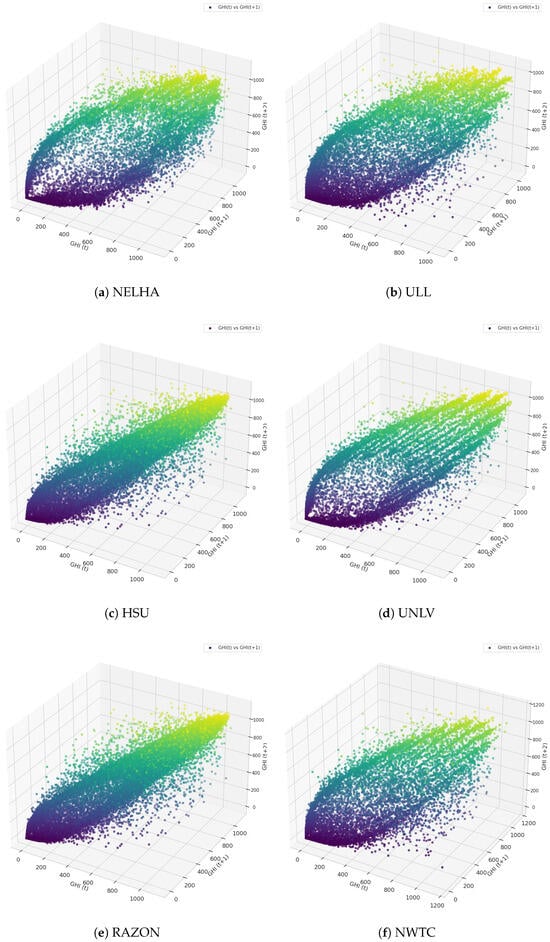
Figure 14.
The 3-D hourly GHI versus GHI and GHI for different stations: (a) NELHA, (b) ULL, (c) HSU, (d) UNLV, (e) RAZON, and (f) NWTC.
3.4. UNLV Station Use Case
As previously shown, the UNLV station achieved the lowest RMSE and the second highest with the MLP model for both 30 min- and 1 h-ahead forecasting. Additionally, it was demonstrated that the model’s performance remains stable for predicting GHI across different shift values. Upon examining feature importance across various forecasting horizons in Figure 15, it becomes clear that the same key features consistently contribute to model performance. These features include the azimuth angle, the first and second lagged versions of GHI, airmass, zenith angle, and DNI values. Given their consistent significance, other features can be considered negligible, allowing for optimal predictions using only these six features.
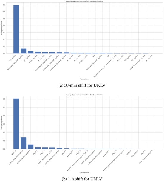
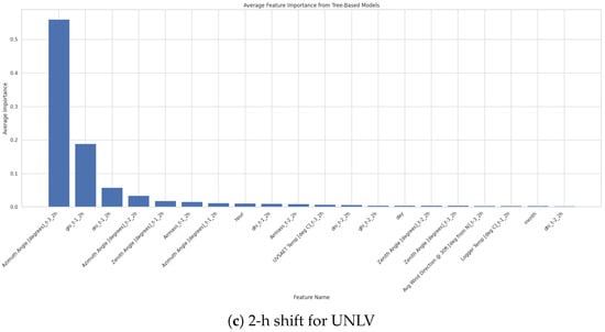
Figure 15.
Sensitivity of regressor performance to time shift and features for UNLV station: (a) 30-min, (b) 1-h, and (c) 2-h shifts.
One of the key factors contributing to the performance observed at the UNLV station is the inherent variation in the GHI, as illustrated in Figure 16. The data reveals a distinct pattern in the GHI readings over the selected years, which appears to be influenced by seasonal effects. Specifically, GHI values tend to rise from March through July and decline during the rest of the year, with relatively stable behavior from December to February. This seasonal trend represents a hidden pattern that can be effectively captured and leveraged by machine learning models, particularly by MLP. MLPs are particularly powerful in detecting such hidden patterns due to their ability to learn complex, non-linear relationships within data. By adjusting their weights through training, MLPs can discern subtle trends and variations in the GHI data that might not be immediately apparent. GHI values generally fall within a range of 10 to 350 on average. While this provides a certain boundary for the MLP’s predictions, it also underscores the model’s capacity to generalize within these limits, ensuring reliable performance across different periods and conditions. The ability of MLPs to detect and utilize these underlying patterns is a significant advantage in making accurate predictions based on GHI data.
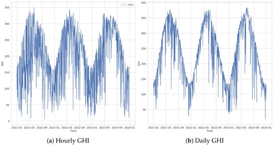
Figure 16.
GHI variations at the UNLV station: (a) hourly and (b) daily.
3.5. Benchmarking with ARIMA and Individual Non-Shifted Features
A comprehensive benchmarking strategy was employed to evaluate the effectiveness of our proposed forecasting solution in comparison with established techniques. As a first step, the results were assessed against those produced by the Seasonal AutoRegressive Integrated Moving Average with Exogenous Regressors (SARIMAX) model. SARIMAX is a well-known statistical time-series model that captures both non-seasonal and seasonal patterns, while also allowing for the inclusion of external covariates. It serves as a strong baseline due to its interpretability and proven performance in univariate forecasting tasks. Subsequently, a second level of benchmarking was conducted using classical machine learning models trained on engineered features, particularly those exhibiting a strong correlation with the target variable, GHI. To ensure a fair and consistent comparison, the same input window size (24 h of historical data) was maintained across all models. This alignment enabled the models to benefit equally from temporal context, avoiding any bias introduced by differing input configurations. The performance of each model was evaluated using standard metrics such as the coefficient of determination and the RMSE, providing a robust and interpretable comparison framework.
It is first evident that the standalone machine learning models incorporating shifted input features (as shown in Figure 17a) exhibit significantly greater robustness and predictive capability than the SARIMAX model. SARIMAX fails to effectively capture the temporal dependencies and complex non-linear dynamics inherent in the meteorological station data. This limitation is quantitatively reflected in its higher RMSE values relative to all the tested standalone models. One contributing factor to this underperformance is SARIMAX’s reliance on substantial historical data to accurately estimate its autoregressive and seasonal parameters, a condition not fully satisfied within the current training regime. In addition to its limited forecasting precision, SARIMAX suffers from considerable computational inefficiency. Training the model on only 20,000 samples required approximately 307.5 s, while the same dataset was processed by the RandomForest in 66.8 s, by XGBoost in 1.08 s, and by CatBoost in 12.0 s. These results clearly raise concerns about SARIMAX’s scalability and suitability for real-time deployment. In a second experiment, we evaluated the impact of using only features with a strong correlation to the target variable. For benchmarking purposes, the UNLV station was selected, as illustrated in Figure 17b. This setup retained a fixed time shift of 30 min. The performance of all models exhibited slight, yet observable degradation. For instance, the MLP model experienced a pronounced increase in RMSE, rising by over 7 units compared to its previous value with temporal shifts (42.82). Additionally, the score fell below the 0.90 threshold, reflecting a degradation of approximately 0.08 relative to its earlier performance (0.98). These results emphasize the critical importance of careful feature selection, particularly in time-series contexts, where lag-based or shift-based variables can significantly enhance model expressiveness. Furthermore, the findings underline important practical considerations regarding the deployment of forecasting models. While classical models like SARIMAX offer strong statistical foundations, their high training time and dependency on extensive data make them less ideal for embedded or resource-constrained environments. In contrast, modern machine learning models, especially tree-based ensembles and neural networks, offer a more favorable balance between accuracy, speed, and scalability for real-time or edge computing scenarios.
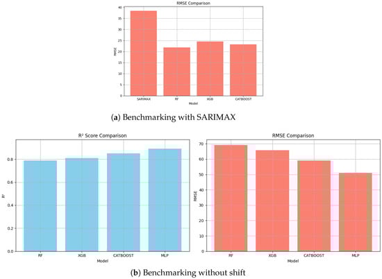
Figure 17.
Model-free benchmark: (a) with SARIMAX and (b) without shift.
3.6. Feature Impacts with SHAP
The SHAP (Shapley Additive Explanations) explainer is a method used to interpret the output of machine learning models by breaking down and attributing the contribution of each feature to the model’s predictions. SHAP values are based on cooperative game theory and the concept of Shapley values, which provide a way to fairly allocate the “payout” (in this context, the prediction) among all features (players) by considering all possible combinations of features [30]. In this context, this explainer was used to understand the impact of features within each station and how they contribute to the model’s performance in predicting the targeted GHI. In each station, the features were analyzed for the 30-min shift, as it was the best horizon for prediction and had the least RMSE observed. Figure 18 and Figure 19 provide the analysis in each station. Analyzing the impactful features reveals that, for all stations, the lagged version of GHI up to 30 min is the most significant feature. While most stations show that only two or three features have the most noticeable impact, the UNLV station stands out with at least six impactful features. These features primarily include the shifted values of global UVA up to 1 h, airmass, the GHI shifted values up to 1 h, and the zenith and azimuth angles. This indicates that including these feature values at the UNLV station could be beneficial for the trained models. Another observation from the SHAP explanations is that it is not necessary to use data from periods far in the past. The explanations show that a maximum lag of 1.5 to 2 h is sufficient for accurate predictions.
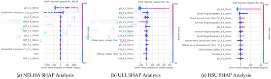
Figure 18.
SHAP feature effects on predictions: (a) NELHA, (b) ULL, and (c) HSU.
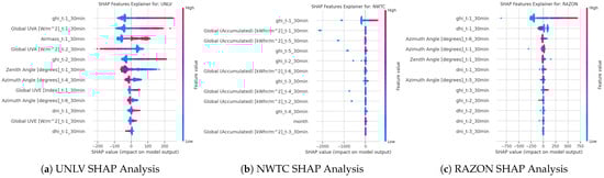
Figure 19.
SHAP feature effects on predictions: (a) UNLV, (b) NWTC, and (c) RAZON.
In addition, from a logical and physical standpoint, it is well-established that features correlated with GHI are inherently linked to both DNI and DHI, given their mutual dependence on solar geometry and atmospheric conditions. However, based on our station-specific analysis, it is evident that the available features vary significantly across different stations. This heterogeneity poses a challenge in establishing a consistent and robust set of predictors for GHI across all sites. While some features, such as the solar zenith and azimuth angles, may be common across stations, their relative contribution to GHI prediction appears limited when compared to that of the lagged GHI values. Our analysis shows that the predictive importance of lagged GHI values decreases as the lag duration increases, which is consistent with the autocorrelation and partial autocorrelation patterns observed in our preliminary time-series analysis. To this end, we primarily rely on the first two lagged values of GHI (i.e., and ) as key features for forecasting. This decision is further supported by the SHAP analysis illustrated in Figure 20, which clearly shows a strong contribution from the first lag, with a noticeably diminished impact from the second lag. These findings are aligned with the earlier SHAP-based feature importance assessments. Moreover, other meteorological variables, such as airmass, though considered in the initial set of features, were found to have minimal influence relative to the lagged GHI values. For this reason, and to reduce model complexity while maintaining interpretability and generalizability across stations, we focused exclusively on using lagged GHI values as predictors in our modeling approach.
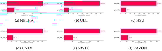
Figure 20.
Overview of shift-degree impact on GHI and related features.
4. Conclusions
This study used a three-year dataset of solar irradiance data collected from six distinct photovoltaic stations. The primary objective was to evaluate the feasibility of developing a consensus among various machine learning models regarding optimal shared features for predicting GHI across multiple sites. To achieve this, a 30-min shift in data was utilized based on a thorough analysis of ACF and PACF, which indicated a strong correlation between each GHI value and its value from 30 min before. The analysis identified that the DNI, DHI, as well as the temperature of the solar panels and related components (primarily CR variants), are critical features for predicting GHI. Subsequently, predictions of GHI were made using data from the six stations, primarily employing tree-based machine learning algorithms and ensemble learners. The results demonstrated that the values exceeded 95% at all six stations and reached 99% for the NWTC station. The RAZON station was an exception, where the metric did not exceed 90%. Specifically, GBR was found to be powerful for NELHA, NWTC, and RAZON, while the MLP performed well for both ULL and UNLV. Finally, CatBoost was the best performer for HSU. The effect of time-shifting values was also evaluated, revealing that with larger shifts, the results deteriorated. MLP emerged as the best model for larger shifting values. It was found that the common lagged GHI values are the most impactful features for predicting the target, along with other features such as solar panel parameters (especially those linked to temperature and ambient conditions), zenith and azimuth angles, and the components of GHI, such as DNI and DHI. These findings underscore the effectiveness of different machine learning models tailored to each station’s specific data characteristics. Although we experimented with a unified stacking ensemble to explore potential gains in cross-site generalizability, the observed performance variability between stations reveals a more fundamental insight: local site characteristics, such as sensor calibration, geographic features, and weather dynamics, heavily influence forecasting accuracy. Thus, our findings reaffirm that site-specific models remain more effective under current data constraints and that achieving universal generalization remains a challenging and open research problem. Nevertheless, the stacking strategy still holds promise as a flexible integration framework, especially if combined with domain adaptation techniques in future work.
Author Contributions
Conceptualization, H.N.N., Z.A., O.S., and K.C.; methodology, H.N.N. and Z.A.; software, H.N.N. and Z.A.; validation, H.N.N., Z.A., O.S., and K.C.; formal analysis, H.N.N., Z.A., O.S., and K.C.; writing—original draft preparation, H.N.N. and Z.A.; writing—review and editing, O.S. and K.C.; visualization, Z.A.; supervision, H.N.N. and K.C.; project administration, H.N.N. All authors have read and agreed to the published version of the manuscript.
Funding
This paper was supported by funds from the Bourgogne-Franche-Comté Region (AAP Région 2022 dispositif ANER-IA Limentaire project) and the EIPHI Graduate School (contract “ANR-17-EURE-0002”).
Data Availability Statement
The data presented in this study are openly available in MIDC RAW DATA API.
Conflicts of Interest
Dr. Ola Salman was employed by the company “DeepVu, USA”. The remaining authors declare that the research was conducted in the absence of any commercial or financial relationships that could be construed as a potential conflict of interest.
Appendix A. Tuned Hyperparameters for Benchmark Models
To ensure a fair and optimized evaluation, each machine learning model was tuned using the Optuna optimization framework with the Tree-structured Parzen Estimator (TPE) sampler and 50 trials. The starting and best values are given in Table A1. All models were evaluated using five-fold cross-validation with the mean squared error as the objective function. The final hyperparameters were used for performance comparison based on R2, RMSE, MAE, MAPE, median absolute error, and D2 metrics.
Table A1.
Starting and best hyperparameters for each model from Optuna tuning.
Table A1.
Starting and best hyperparameters for each model from Optuna tuning.
| Model | Best Hyperparameters |
|---|---|
| RandomForest Regressor | n_estimators = [10, 200], max_depth: [10–18] |
| GradientBoosting Regressor | n_estimators = [10–150], learning_rate: 0.05, max_depth: 10 |
| Decision Tree Regressor | max_depth: [3–12] |
| MLP Regressor | hidden_layer_sizes: (100, 100), learning_rate_init: 0.001 |
| CatBoost Regressor | learning_rate = 0.03, depth: 6 |
| LightGBM Regressor | n_estimators: [50, 200], learning_rate: 0.02, num_leaves: [10–40] |
| XGBoost Regressor | n_estimators: [50, 180], learning_rate: 0.07, max_depth: 9 |
References
- Wang, F.; Harindintwali, J.D.; Wei, K.; Shan, Y.; Mi, Z.; Costello, M.J.; Grunwald, S.; Feng, Z.; Wang, F.; Guo, Y.; et al. Climate change: Strategies for mitigation and adaptation. Innov. Geosci. 2023, 1, 100015-61. [Google Scholar] [CrossRef]
- Agreement, P. Paris agreement. In Report of the Conference of the Parties to the United Nations Framework Convention on Climate Change (21st Session, 2015: Paris); Retrieved December; HeinOnline: Getzville, NY, USA, 2015; Volume 4, p. 2. [Google Scholar]
- Diagne, M.; David, M.; Lauret, P.; Boland, J.; Schmutz, N. Review of solar irradiance forecasting methods and a proposition for small-scale insular grids. Renew. Sustain. Energy Rev. 2013, 27, 65–76. [Google Scholar] [CrossRef]
- Allal, Z.; Noura, H.N.; Chahine, K. Machine Learning Algorithms for Solar Irradiance Prediction: A Recent Comparative Study. e-Prime-Adv. Electr. Eng. Electron. Energy 2024, 7, 100453. [Google Scholar] [CrossRef]
- Abdel-Nasser, M.; Mahmoud, K.; Lehtonen, M. Reliable solar irradiance forecasting approach based on choquet integral and deep LSTMs. IEEE Trans. Ind. Inform. 2020, 17, 1873–1881. [Google Scholar] [CrossRef]
- Wang, F.; Mi, Z.; Su, S.; Zhao, H. Short-term solar irradiance forecasting model based on artificial neural network using statistical feature parameters. Energies 2012, 5, 1355–1370. [Google Scholar] [CrossRef]
- Ramadhan, R.A.; Heatubun, Y.R.; Tan, S.F.; Lee, H.J. Comparison of physical and machine learning models for estimating solar irradiance and photovoltaic power. Renew. Energy 2021, 178, 1006–1019. [Google Scholar] [CrossRef]
- Haider, S.A.; Sajid, M.; Sajid, H.; Uddin, E.; Ayaz, Y. Deep learning and statistical methods for short-and long-term solar irradiance forecasting for Islamabad. Renew. Energy 2022, 198, 51–60. [Google Scholar] [CrossRef]
- Miller, S.D.; Rogers, M.A.; Haynes, J.M.; Sengupta, M.; Heidinger, A.K. Short-term solar irradiance forecasting via satellite/model coupling. Sol. Energy 2018, 168, 102–117. [Google Scholar] [CrossRef]
- Verbois, H.; Saint-Drenan, Y.M.; Thiery, A.; Blanc, P. Statistical learning for NWP post-processing: A benchmark for solar irradiance forecasting. Sol. Energy 2022, 238, 132–149. [Google Scholar] [CrossRef]
- Zambrano, A.F.; Giraldo, L.F. Solar irradiance forecasting models without on-site training measurements. Renew. Energy 2020, 152, 557–566. [Google Scholar] [CrossRef]
- Wang, F.; Xuan, Z.; Zhen, Z.; Li, Y.; Li, K.; Zhao, L.; Shafie-khah, M.; Catalão, J.P. A minutely solar irradiance forecasting method based on real-time sky image-irradiance mapping model. Energy Convers. Manag. 2020, 220, 113075. [Google Scholar] [CrossRef]
- Rohani, A.; Taki, M.; Abdollahpour, M. A novel soft computing model (Gaussian process regression with K-fold cross validation) for daily and monthly solar radiation forecasting (Part: I). Renew. Energy 2018, 115, 411–422. [Google Scholar] [CrossRef]
- Li, J.; Ward, J.K.; Tong, J.; Collins, L.; Platt, G. Machine learning for solar irradiance forecasting of photovoltaic system. Renew. Energy 2016, 90, 542–553. [Google Scholar] [CrossRef]
- Alzahrani, A.; Shamsi, P.; Dagli, C.; Ferdowsi, M. Solar irradiance forecasting using deep neural networks. Procedia Comput. Sci. 2017, 114, 304–313. [Google Scholar] [CrossRef]
- Yahya, N.W.; Prasad, D.R.; Sathiyamoorthy, D.; Pendyala, R. Prospects and roadmaps for harvesting solar thermal power in tropical Brunei Darussalam. Int. J. Glob. Energy Issues 2021, 43, 616–642. [Google Scholar] [CrossRef]
- Chu, Y.; Pedro, H.T.; Li, M.; Coimbra, C.F. Real-time forecasting of solar irradiance ramps with smart image processing. Sol. Energy 2015, 114, 91–104. [Google Scholar] [CrossRef]
- Pazikadin, A.R.; Rifai, D.; Ali, K.; Malik, M.Z.; Abdalla, A.N.; Faraj, M.A. Solar irradiance measurement instrumentation and power solar generation forecasting based on Artificial Neural Networks (ANN): A review of five years research trend. Sci. Total Environ. 2020, 715, 136848. [Google Scholar] [CrossRef]
- Kumari, P.; Toshniwal, D. Extreme gradient boosting and deep neural network based ensemble learning approach to forecast hourly solar irradiance. J. Clean. Prod. 2021, 279, 123285. [Google Scholar] [CrossRef]
- Bamisile, O.; Oluwasanmi, A.; Ejiyi, C.; Yimen, N.; Obiora, S.; Huang, Q. Comparison of machine learning and deep learning algorithms for hourly global/diffuse solar radiation predictions. Int. J. Energy Res. 2022, 46, 10052–10073. [Google Scholar] [CrossRef]
- Gürel, A.E.; Ağbulut, Ü.; Biçen, Y. Assessment of machine learning, time series, response surface methodology and empirical models in prediction of global solar radiation. J. Clean. Prod. 2020, 277, 122353. [Google Scholar] [CrossRef]
- Ikram, R.M.A.; Dai, H.L.; Ewees, A.A.; Shiri, J.; Kisi, O.; Zounemat-Kermani, M. Application of improved version of multi verse optimizer algorithm for modeling solar radiation. Energy Rep. 2022, 8, 12063–12080. [Google Scholar] [CrossRef]
- Husein, M.; Chung, I.Y. Day-ahead solar irradiance forecasting for microgrids using a long short-term memory recurrent neural network: A deep learning approach. Energies 2019, 12, 1856. [Google Scholar] [CrossRef]
- Sansine, V.; Ortega, P.; Hissel, D.; Hopuare, M. Solar Irradiance Probabilistic Forecasting Using Machine Learning, Metaheuristic Models and Numerical Weather Predictions. Sustainability 2022, 14, 15260. [Google Scholar] [CrossRef]
- Measurement and Instrumentation Data Center (MIDC). MIDC Raw Data API Documentation. 2024. Available online: https://midcdmz.nrel.gov/apps/data_api_doc.pl?_idtextlist (accessed on 19 July 2024).
- Pedregosa, F.; Varoquaux, G.; Gramfort, A.; Michel, V.; Thirion, B.; Grisel, O.; Blondel, M.; Prettenhofer, P.; Weiss, R.; Dubourg, V.; et al. Scikit-Learn: Machine Learning in Python. 2011. Available online: https://scikit-learn.org/stable/ (accessed on 20 July 2024).
- Nemeth, M.; Borkin, D.; Michalconok, G. The comparison of machine-learning methods XGBoost and LightGBM to predict energy development. In Proceedings of the Computational Statistics and Mathematical Modeling Methods in Intelligent Systems: Proceedings of 3rd Computational Methods in Systems and Software 2019; Springer: Cham, Switzerland, 2019; Volume 23, pp. 208–215. [Google Scholar]
- Dasi, H.; Ying, Z.; Yang, B. Predicting the consumed heating energy at residential buildings using a combination of categorical boosting (CatBoost) and Meta heuristics algorithms. J. Build. Eng. 2023, 71, 106584. [Google Scholar] [CrossRef]
- Ahmad, T.; Manzoor, S.; Zhang, D. Forecasting high penetration of solar and wind power in the smart grid environment using robust ensemble learning approach for large-dimensional data. Sustain. Cities Soc. 2021, 75, 103269. [Google Scholar] [CrossRef]
- Lundberg, S.M.; Lee, S.I. SHAP (SHapley Additive exPlanations). 2023. Available online: https://shap.readthedocs.io/en/latest/ (accessed on 30 July 2024).
Disclaimer/Publisher’s Note: The statements, opinions and data contained in all publications are solely those of the individual author(s) and contributor(s) and not of MDPI and/or the editor(s). MDPI and/or the editor(s) disclaim responsibility for any injury to people or property resulting from any ideas, methods, instructions or products referred to in the content. |
© 2025 by the authors. Licensee MDPI, Basel, Switzerland. This article is an open access article distributed under the terms and conditions of the Creative Commons Attribution (CC BY) license (https://creativecommons.org/licenses/by/4.0/).